Hamilton Approach to QCD in Coulomb Gauge: Finite Temperatures and Chiral Symmetry Breaking

Abstract:

I will review results obtained recently within the Hamilton approach to QCD in Coulomb gauge. The focus will be on finite-temperature Yang–Mills theory and chiral symmetry breaking in QCD.

1 Introduction

In this talk I will give an overview over recent results obtained within the Hamiltonian approach to QCD in Coulomb gauge. I will focus on the extension of this approach to finite temperatures and to the inclusion of quarks. My main interest here will be the finite-temperature deconfinement phase transition and the spontaneous breaking of chiral symmetry.

Going to Weyl gauge $A_{0}=0$ canonical quantization of Yang–Mills theory yields the following Hamiltonian

$$H=\frac{1}{2}\int\left(\vec{\Pi}^{2}+\vec{B}^{2}\right).$$ (1)

Here $\vec{\Pi}=\delta/i\delta\vec{A}$ is the canonical momentum operator and $\vec{B}$ is the non-Abelian magnetic field. The Yang–Mills Hamiltonian (1) is invariant under spatial (time-independent) gauge transformations. A quantity of central interest in quantum field theory is the vacuum wave functional, by means of which all correlation functions can be evaluated. This quantity is obtained by solving the Schrödinger equation

$$H\psi=E\psi$$ (2)

for the lowest energy eigenstate. There have been various attempts to solve the Yang–Mills Schrödinger equation (2) directly for gauge invariant wave functionals, in particular in $D=2+1$, see Ref. [1] and references therein. One can give arguments that the Yang–Mills vacuum wave functional (in $D=3+1$) can be approximated in the low-energy regime by [2]

$$\psi[A]=\exp\left[-\frac{1}{2}\int F^{2}_{ij}\right].$$ (3)

So far one has not succeeded in determining the Yang–Mills vacuum wave functional in a gauge invariant way. A much more convenient way is to fix the gauge and for the purpose of Hamiltonian Yang–Mills theory Coulomb gauge is, in particular, convenient. The prize one pays is that the Hamiltonian is more complicated. In Coulomb gauge the Yang–Mills Hamiltonian is given by [3]

$$H=\frac{1}{2}\int\left(J^{-1}\vec{\Pi}^{\perp}J\vec{\Pi}^{\perp}+\vec{B}^{2}\right)+H_{C}\,,$$ (4)

where $J=\operatorname{Det}(-\hat{D}\partial)$ is the Faddeev–Popov determinant with $\hat{D}=\partial+g\hat{A}$, $\hat{A}^{ab}=f^{acb}A^{c}$ being the covariant derivative in the adjoint representation. Furthermore,

$$H_{C}=\frac{1}{2}\int J^{-1}\vec{\Pi}^{\parallel}J\vec{\Pi}^{\parallel}=\frac{g^{2}}{2}\int J^{-1}\rho(-\hat{D}\partial)^{-1}(-\partial^{2})(-\hat{D}\partial)^{-1}J\rho$$ (5)

is the Coulomb Hamiltonian, which arises from solving Gauss’s law (which is a constraint to the wave functional to guarantee gauge invariance) for the longitudinal momentum operator $\vec{\Pi}^{\parallel}$. In Eq. (5), $\rho=\rho_{gl}+\rho_{m}$ is the total color charge, which contains beside the charge of the Yang–Mills field $\rho_{gl}=-\hat{\vec{A}}\vec{\Pi}$ also the charge of the matter fields $\rho_{m}$. By resolving Gauss’s law gauge invariance has been fully taken into account and in Coulomb gauge each functional of the transverse gluon field $A^{\perp}$, $\partial A^{\perp}=0$ is, in principle, a physical wave functional. Note that in the canonical quantization of Yang–Mills theory the gauge field figures as the coordinate, and the transition to Coulomb gauge implies a transition to curvilinear coordinates. Accordingly, the kinetic piece of the Yang–Mills Hamiltonian [the first term in Eq. (4)] resembles the Laplacian in curvilinear coordinates. In the scalar product of the Yang–Mills wave functionals the transition to Coulomb gauge can be accomplished by using the standard Faddeev–Popov method, which introduces the Faddeev–Popov determinant also in the integration measure

$$\langle\phi|\dots|\psi\rangle=\int DA\>J(A)\,\phi^{*}(A)\dots\psi(A).$$ (6)

2 Zero-temperature Yang–Mills theory

One can solve the Yang–Mills Schrödinger equation in perturbation theory by expanding the Hamiltonian and the wave functional in powers of the coupling constant $g$, applying standard Rayleigh–Schrödinger perturbation theory [4]. From the Coulomb term (5), which is order $g^{2}$, one can extract the running coupling constant and obtains the same result as in ordinary covariant perturbation theory within the functional integral formulation. We are interested here, however, in a non-perturbative solution of the Yang–Mills Schrödinger equation and for this purpose we exploit the variational approach using Gaussian type wave functionals. The first variational calculations in Coulomb gauge were performed in Ref. [5] and later on in Ref. [6]. Our approach [7] differs from previous variational calculations in Coulomb gauge in the ansatz of the vacuum wave functional, in the treatment of the Faddeev–Popov determinant (treated fully in our approach and at least partially neglected in previous approaches) and in the renormalization, for more details see Sect. IID of Ref. [1].

The variational approach developed in Tübingen uses the trial ansatz for the vacuum wave functional [7]

$$\psi(A)=\frac{1}{\sqrt{\operatorname{Det}(-\hat{D}\partial)}}\exp\left[-\frac{1}{2}\int A\omega A\right],$$ (7)

which contains besides the exponential the inverse square root of the Fadeev–Popov determined. This has the advantage that in expectation values the Faddeev–Popov determinant in the integration measure, see Eq. (6), is cancelled. Furthermore, the static gluon propagator is with this wave functional given by the inverse of the variational kernel $\omega$

$$\langle AA\rangle=(2\omega)^{-1},$$ (8)

which shows that $\omega$ has the meaning of the gluon energy. Minimizing the vacuum expectation value of the Hamiltonian, $\langle\psi|H|\psi\rangle\to\mathrm{min}$, one finds [8] for the gluon energy $\omega$ the result shown in Fig. 2 (dashed line). At large momenta it behaves like the photon energy $\omega(k\to\infty)\sim k$ and is infrared divergent $\omega(k\to 0)\sim 1/k$. This, of course, is the manifestation of the confinement of gluons. Figure 2 shows the lattice results [9] for the gluon propagator (8), which can be fitted by Gribov’s formula.

Figure 1: Comparison of the gluon propagator $1/(2\omega)$ with Gaussian [8] (dashed line) and non-Gaussian [10] (full line) functional to the lattice data [9].

Figure 2: Form factor of the three-gluon vertex for orthogonal momenta and comparison to lattice data for the 3-dimensional Landau-gauge vertex [11].

$$\omega(k)=\sqrt{k^{2}+\frac{M^{4}}{k^{2}}}$$ (9)

with the effective mass $M\approx 880$ MeV. Also shown in this figure is the result of the variational calculation [8]: as can be seen the gluon propagator obtained from the variational calculation agrees quite well with the lattice data in the infrared and the ultraviolet, while there is some missing strength in the mid-momentum regime around 1 GeV. This can be traced back to the absence of the gluon loop, which escapes the variational calculation with the Gaussian type of ansatz (7). In Ref. [10] the variational approach was extended to non-Gaussian wave functionals including up to quartic terms in the gauge field

$$|\psi[A]|^{2}=\exp(-S[A]),\qquad S[A]=\int\omega A^{2}+\frac{1}{3!}\int\gamma^{(3)}A^{3}+\frac{1}{4!}\int\gamma^{(4)}A^{4}.$$ (10)

To capture the gluon loop in the variational calculation one needs to include at least the three-gluon term $\gamma^{(3)}$ in the exponent of the wave functional. Then one finds the static gluon propagator shown in Fig. 2 (full line), which gives a substantial improvement compared to the propagator obtained with the Gaussian trial wave functional. Figure 2 shows the result for the three-gluon vertex. Also shown are the lattice result for the three-gluon vertex calculated in 3-dimensional Landau gauge Yang–Mills theory [11]. This theory corresponds to the use of the approximate wave functional (3) in $3+1$ dimensional Yang–Mills theory in the Hamiltonian approach. Since the expression (3) represents a good approximation to the true Yang–Mills wave functional in the low-momentum regime (see Ref. [12]) we expect the 3-dimensional Landau gauge lattice result to agree well with the static three-gluon vertex in $D=3+1$ Yang–Mills theory. Indeed we find a quite reasonable agreement between the result of the variational calculation and the lattice data in the infrared.

The above represented solution correspond to the so-called critical (or scaling) solution, where the horizon condition $d^{-1}(k=0)=0$ was assumed for the ghost form factor $d(k)$ defined by the ghost propagator

$$\langle(-\hat{D}\partial)^{-1}\rangle=d(k)/k^{2}.$$ (11)

Figure 3 shows the result of the variational calculation for the gluon energy (shown already in Fig. 2) and the ghost form factor of the full variational calculation and the one with the Coulomb term of the Hamiltonian, Eq. (5), excluded. One observes that the effect of the Coulomb term is very small. We will therefore neglect this term in subsequent numerical calculations.

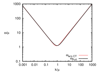
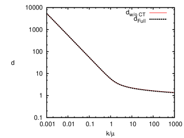
Figure 3: The gluon energy (left panel) and the ghost form factor (right panel) with and without the Coulomb term.

3 Finite-temperature Yang–Mills theory

To extend Yang–Mills theory to finite temperatures [13, 14] we consider the grand canonical ensemble with vanishing chemical potential, which is defined by the density matrix

$$D=\exp\bigl{[}-H/(k_{\textsc{b}}T)\bigr{]},$$ (12)

where $k_{\textsc{b}}$ is Boltzmann constant. For the evaluation of the thermal averages

$$\langle\dots\rangle_{T}=\frac{\operatorname{Tr}(D\dots)}{\operatorname{Tr}D}$$ (13)

we need a complete basis of the gluonic Fock space, which we choose in analogy to the ground state wave functional (7) in the form

$$|\tilde{k}\rangle=\frac{1}{\sqrt{\operatorname{Det}(-\hat{D}\partial)}}|k\rangle,$$ (14)

where the $|k\rangle$ form a complete set of states of the gluonic Fock space, which we choose in the following way: we decompose the gauge field (in momentum space) in terms of creation and annihilation operators

$$A(k)=\frac{1}{\sqrt{2\omega(k)}}\left(a(k)+a^{\dagger}(-k)\right),$$ (15)

where $\omega(k)$ is an arbitrary (positive definite) kernel. Defining the vacuum state $|k=0\rangle$ by

$$a(k)|0\rangle=0$$ (16)

this state becomes in coordinate representation

$$\langle A|0\rangle=\exp\left(-\frac{1}{2}\int A\omega A\right).$$ (17)

A complete basis of the gluonic Fock space is then given by

$$|0\rangle,\quad a^{\dagger}(k)|0\rangle,\quad a^{\dagger}(k)a^{\dagger}(k^{\prime})|0\rangle,\quad\dots$$ (18)

The exact density matrix (12) is too difficult to handle given the complicated form of the Yang–Mills Hamiltonian. For this purpose we replace the Yang–Mills Hamiltonian in the density matrix by a single-particle Hamiltonian

$$D=\exp\bigl{[}-h/(k_{\textsc{b}}T)\bigr{]},\qquad h=\int\mathop{\mathrm{d}\mkern-5.5mu\mathchar 22\relax}{k}\>\Omega(k)\,a^{\dagger}(k)\,a(k),\qquad\mathop{\mathrm{d}\mkern-5.5mu\mathchar 22\relax}{k}\equiv\mathrm{d}^{3}k/(2\pi)^{3}.$$ (19)

Since $h$ is a single-particle Hamiltonian the thermal averages (13) with the density matrix (19) can be worked out by using Wick’s theorem. For the gluonic occupation numbers one finds

$$\langle a(\vec{k})a^{\dagger}(\vec{k}^{\prime})\rangle_{T}=(2\pi)^{3}\delta(\vec{k}-\vec{k}^{\prime})n(k),\qquad\text{with}\qquad n(k)=\bigl{[}\exp\bigl{(}\Omega(k)/(k_{\textsc{b}}T)\bigr{)}-1\bigr{]}^{-1},$$ (20)

which are the usual Bose occupation numbers with $\Omega(k)$ representing the single-particle energies. By means of Wick’s theorem all thermal averages can then be expressed in terms of the gluon propagator

$$\langle A(\vec{k})A(\vec{k}^{\prime})\rangle_{T}=(2\pi)^{3}\delta(\vec{k}+\vec{k}^{\prime})\bigl{(}1+2n(k)\bigr{)}/\bigl{(}2\omega(k)\bigr{)}.$$ (21)

From the density matrix (19) we find the entropy $S$ and the free energy $F$

$$S=-k_{\textsc{b}}\operatorname{Tr}D\ln D,\qquad F=\langle H\rangle_{T}-TS.$$ (22)

So far the two kernels $\Omega(k)$, entering the density matrix (19), and $\omega(k)$, entering our basis states (17), are completely arbitrary. We now determine $\Omega(k)$ by minimizing the free energy (22). Instead of taking the variation with respect to $\Omega(k)$ it is more convenient to take the variation with respect to the finite temperature occupation numbers $n(k)$ (20), which is equivalent since $n(k)$ is a monotonic function of $\Omega(k)$. This yields

$$\Omega(k)=\frac{\delta e[n,\omega]}{\delta n(k)}\,,$$ (23)

where $e[n,\omega]=\langle H\rangle_{T}/\bigl{(}2(N^{2}_{\mathrm{c}}-1)\cdot V\bigr{)}$ is the energy density per gluonic degree of freedom ($V$ is the spatial volume). From the analogy with Landau’s liquid Fermi theory we identify $\Omega(k)$ as a quasi-gluon energy. Evaluating the thermal expectation value of the Yang–Mills Hamiltonian $\langle H\rangle_{T}$ up to two loops one finds for the quasi-gluon energy

$$\frac{\Omega(k)}{\omega(k)}=1+\frac{g^{2}N_{\mathrm{c}}}{4}\int\mathop{\mathrm{d}\mkern-5.5mu\mathchar 22\relax}{q}\>F(\vec{k}-\vec{q})\>\frac{1+(\hat{k}\cdot\hat{q})^{2}}{\omega(q)}\>\bigl{[}1+2n(q)\bigr{]}.$$ (24)

The kernel $\omega(k)$ can be chosen, in principle, completely arbitrary (except that it has to be positive definite) and the results of our variational calculation should not depend on the choice of $\omega(k)$. However, since we have introduced approximations (calculating the energy up to two loops) our results do depend on $\omega(k)$. The best we can do is to vary the free energy $F$ Eq. (22) with respect to $\omega(k)$. This guarantees that the free energy is at least to first order independent of $\omega(k)$. From $\delta F/\delta\omega(k)=0$ we find the gap equation

$$\omega^{2}(k)=k^{2}+\chi^{2}(k)+I_{\text{tad}}[n]+I_{\text{c}}[n](k),$$ (25)

where $\chi(k)$ is the ghost loop, $I_{\text{tad}}[n]$ is the tadpole and $I_{\text{c}}[n](k)$ the one gluon-loop contribution from the Coulomb term, see Fig. 4.

(a)

(b)

(c)

Figure 4: Diagrammatic representation of the contributions to the gap equation: (a) full ghost loop, (b) tadpole, (c) one-gluon loop contribution from the Coulomb term. Small black dots and open circles represent, respectively, bare and full vertices of the Hamiltonian; the double line denotes the Coulomb kernel.

The finite-temperature modifications arise exclusively from the finite-temperature part of the gluon propagator, Eq. (21), which depends on the occupation number $n(k)$. The finite-temperature modifications are all ultraviolet finite so the renormalization of the gap and Dyson–Schwinger equations can be done in exactly the same way as at zero temperature, see Ref. [15]. The gap equation has to be solved together with the Dyson–Schwinger equation for the ghost propagator, which is illustrated in Fig. 5. This equation is the same one as at zero temperature except that the gluon propagator is replaced by its finite-temperature counterpart (21). As we have illustrated above for zero temperature, the Coulomb term of the Yang–Mills Hamiltonian does barely influence the ghost and gluon propagator. Therefore we will ignore the Coulomb term in the following. Neglecting the Coulomb term leads to substantial simplifications [14]. The quasi-gluon energy $\Omega(k)$ of the density matrix (19) and the kernel $\omega(k)$ of the vacuum wave functional (17) become then identical. Furthermore, the ghost Dyson–Schwinger equations and the gap equation then decouple from the Dyson-Schwinger equation for the Coulomb form factor [7].

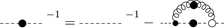
Figure 5: Diagrammatic representation of the ghost DSE.

4 Infrared analysis

Before we present the numerical results let us summarize the results of an infrared analysis for the remaining gap and ghost Dyson-Schwinger equations. Let us first recapitulate the result of the infrared analysis at zero temperatures [16].

For the infrared analysis we assume power-law behaviours of the propagators involved

$$\omega(p\to 0)=A/p^{\alpha},\qquad d(p\to 0)=B/p^{\beta}.$$ (26)

Assuming the horizon condition $d^{-1}(p=0)=0$, which implies $\beta>0$, we find from the ghost DSE the sum rule

$$\alpha=2\beta+2-d,$$ (27)

where $d$ is the number of spatial dimensions. For Coulomb gauge in $d=3$ we obtain $\alpha=2\beta-1$, and including also the gap equation one finds the following two solutions

$$\beta=1\;(1.001),\qquad\beta=0.796\;(0.794),$$ (28)

where the results from the numerical evaluation are given in the bracket. In $d=2$ dimensions one finds a single solution, which within the angular approximation is given by

$$\beta=0.5\;(0.45)$$ (29)

while without the angular approximation one finds $\beta=0.4$.

At arbitrary finite temperature the infrared analysis cannot be carried out since the gluon energy $\Omega(k)=\omega(k)$ enters the thermal occupation numbers $n(k)$, Eq. (20), in the exponent. However, at very high temperatures we can expand this exponent and the occupation numbers reduce to

$$n(k)=k_{\textsc{b}}T/\omega(k).$$ (30)

Then $\omega(k)$ enters only as power in the gap and DSE and we can carry out the infrared analysis in the standard fashion. One finds the same sum rule Eq. (27) as at zero temperature. However, one obtains only a single solution for the infrared exponent

$$\beta=1/2,\qquad\alpha=0.$$ (31)

This is the infrared exponent for the ghost in $d=2$ dimensions, which reflects the fact that at high temperature a dimensional reduction to the $2+1$-dimensional theory occurs.

5 Numerical results

Figure 7 shows the ghost infrared exponent $\beta$ determined from the numerical solutions as function of the temperature. As one observes the infrared exponent stays constant below a critical temperature where it suddenly drops and approaches the value $\beta=1/2$ for high temperatures, in agreement with the infrared analysis. Both zero-temperature solutions, $\beta=1$ and $\beta=0.796$, convert to the same high-temperature solution. Figures 7 and 9 show the numerical solutions for the ghost form factor and the gluon energy for zero temperature and above the deconfinement temperature. One observes that the infrared behaviour is indeed in accord with the findings of the infrared analysis.

Figure 6: IR exponent of ghost as function of the temperature.

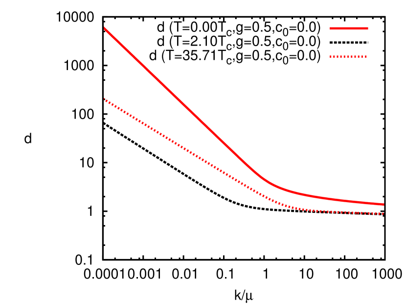
Figure 7: The ghost form factor.

The sudden drop of the infrared exponent of the ghost form factor (see Fig. 7) can be used to define the deconfinement phase transition temperature $T_{c}$. Fitting at $T=0$ the numerical solution for $\omega(k)$ to the lattice gluon propagator [9] to fix the physical scale one finds for the critical temperature of the deconfinement phase transition

$$T_{c}\sim 270\dots 290\mbox{ Mev},$$ (32)

for $SU(2)$, which compares well with the lattice result of $T_{c}=295$ MeV.

Figure 9 shows the infrared mass of the gluon defined by the gluon energy at the numerical infrared scale $\lambda_{\mathrm{IR}}$,

$$m(T)=\omega(k=\lambda_{\mathrm{IR}},T).$$ (33)

This mass behaves similarly as the infrared exponent of the ghost form factor. It stays constant below a critical temperature, where it suddenly drops and after that starts rising linearly with the temperature.

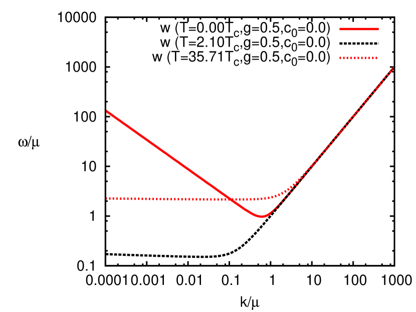
Figure 8: The gluon energy.

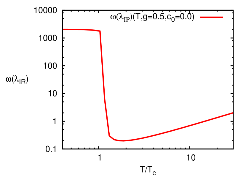
Figure 9: The IR mass of the gluon.

Zooming into the behaviour of $m(T)$ in the transition regime of Fig. 9, see Fig. 11, one finds for the critical exponent of the effective gluon mass defined by

$$m(T)\sim\left(T/T_{c}-1\right)^{-\kappa}$$ (34)

a value of $\kappa\simeq 0.37$. This compares well with the result of $\kappa=0.41$ obtained in Ref. [17], where a quasi-gluon picture has been used to fit the lattice results for the energy density and the pressure, and assuming furthermore input from the $d=3$ Ising model, which is in the same universality class as $SU(2)$ gauge theory.

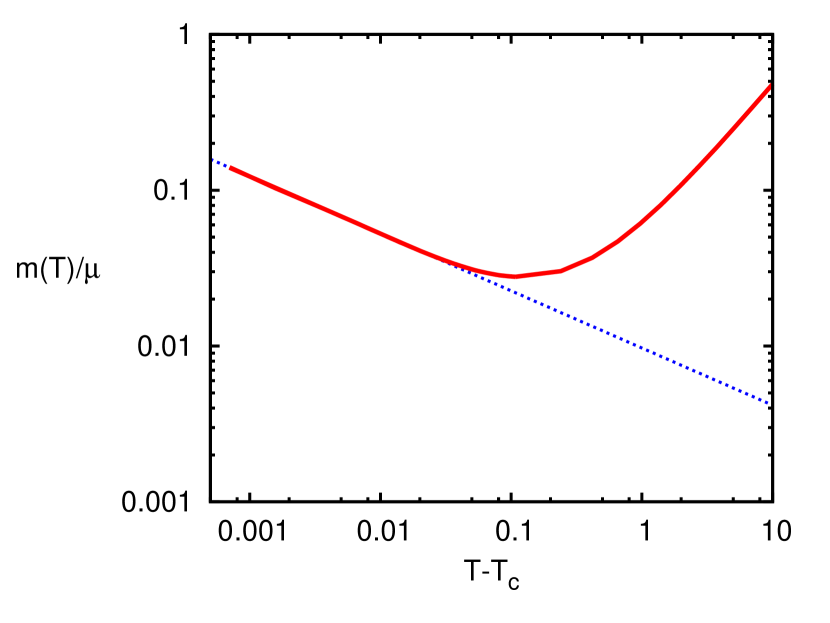
Figure 10: Critical behaviour of the effective gluon mass.

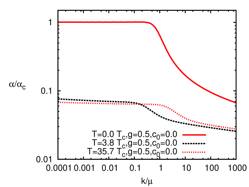
Figure 11: Running coupling constant from the ghost-gluon vertex.

Figure 11 shows the running coupling constant at zero temperature and above the deconfinement phase transition. One observes a substantial reduction of the low energy plateau.

6 Hamiltonian approch to QCD

When the quarks are included the Hamiltonian (4) has to be supplemented by the quark term

$$H_{q}=\int q^{\dagger}(\vec{x})\left[\vec{\alpha}\left(\vec{p}+g\vec{A}\right)+\beta m_{0}\right]q(\vec{x}),$$ (35)

where $q(\vec{x})$ denotes the quark field operator and $m_{0}$ is the current quark mass. Furthermore, the matter charge density in the Coulomb Hamiltonian (5) becomes $\rho^{a}_{m}(x)=q^{\dagger}(x)t^{a}q(x)$, where $t^{a}$ are the generators of the gauge group in the fundamental representation. For the quark sector we use the following ansatz for the vacuum wave functional [18]

$$|\phi\rangle_{\textsc{q}}=\exp\left[\int q^{\dagger}\left(S\beta+V\vec{\alpha}\cdot\vec{A}\right)q\right]|0\rangle,$$ (36)

where $|0\rangle$ is the perturbative quark vacuum state, which describes a system of free quarks with mass $m_{0}$. Furthermore $S$ and $V$ are variational kernels to be determined by minimizing the energy density. For $V=0$ Eq. (36) defines a BCS-type wave functional considered in Ref. [19]. The new important aspect of the wave function (36) is the coupling of the quarks to the gauge field with form factor $V$. Without this term the quark-gluon coupling in the quark Hamiltonian (35) escapes the expectation value. The total QCD wave functional is then given by

$$|\Phi\rangle=|\psi\rangle_{\textsc{ym}}\otimes|\phi\rangle_{\textsc{q}}\,,$$ (37)

where $|\psi\rangle_{\textsc{ym}}$ is the Yang–Mills vacuum wave functional given in Eq. (7). We keep $\omega$ fixed at its form determined from the Yang-Mills sector. We minimize the quark energy $\langle\langle H_{q}\rangle_{\textsc{q}}\rangle_{\textsc{ym}}$ with respect to the kernels $S$ and $V$. The result of this variation is shown in Fig. 13.

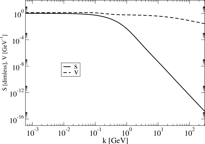
Figure 12: The variational kernels $S$ and $V$.

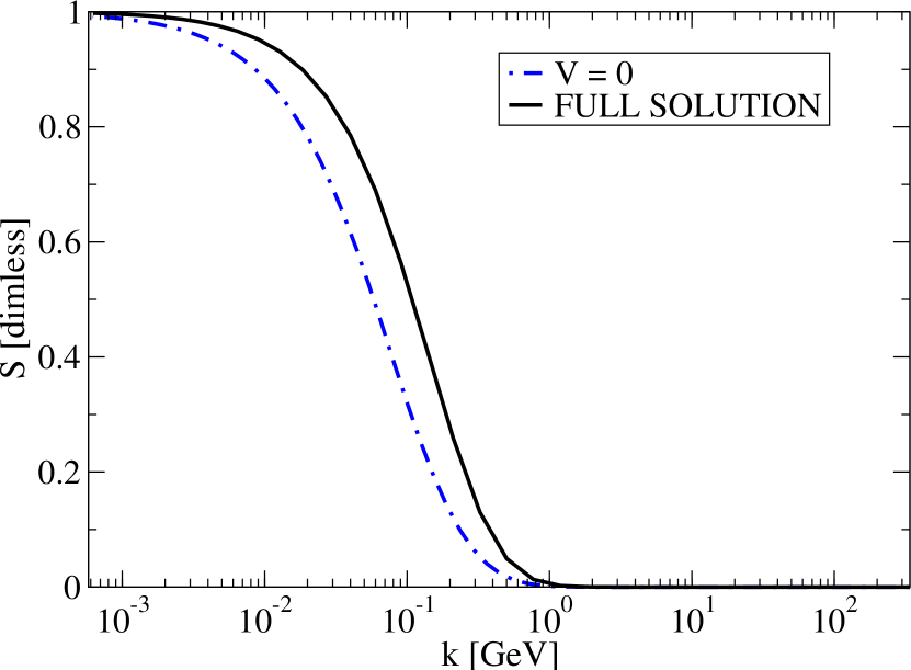
Figure 13: Comparison of scalar kernel $S(k)$ with ($V\neq 0$) and without $(V=0)$ the quark-gluon coupling included.

Figure 13 compares the scalar form factor with and without taking into account the quark-gluon coupling. With the quark-gluon coupling switched off ($V=0$) we find the value for the quark condensate

$$\langle\bar{q}q\rangle=\Bigl{(}-113\mbox{ MeV}\sqrt{\sigma_{\textsc{c}}/\sigma_{\textsc{w}}}\Bigr{)}^{3},$$ (38)

which corresponds to the result of Ref. [19], while with the quark gluon coupling included ($V\neq 0$) we obtain

$$\langle\bar{q}q\rangle=\left(-135\mbox{ MeV}\sqrt{\sigma_{\textsc{c}}/\sigma_{\textsc{w}}}\right)^{3}.$$ (39)

This is an increase of the figure in the bracket by about 20%. In Eqs. (38) and (39) $\sigma_{\textsc{c}}$ and $\sigma_{\textsc{w}}$ denote respectively the Coulomb and Wilsonian string tension. Lattice results show that the ratio of these quantities is given in the range of

$$\sigma_{\textsc{c}}/\sigma_{\textsc{w}}\simeq 2\dots 3.$$ (40)

This implies a quark condensate in the range of

$$\langle\bar{q}q\rangle=(-191\dots 234\mbox{ MeV})^{3},$$ (41)

which compares well with the phenomenological value of

$$\langle\bar{q}q\rangle=(-230\mbox{ MeV})^{3}.$$ (42)

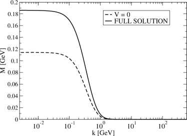
Figure 14: Running quark mass.

Figure 14 shows the dynamical quark mass as a function of the momentum with and without the quark gluon coupling. We observe an essential increase in the quark mass when the coupling of the quarks to the gluons is included. For the constituent quark mass defined by the zero momentum value of the running quark mass $M=M(k=0)$ we obtain without the quark-gluon coupling ($V=0$)

$$M=84\mbox{ MeV}\sqrt{\sigma_{\textsc{c}}/\sigma_{\textsc{w}}}$$ (43)

and with the quark-gluon coupling included ($V\neq 0$)

$$M=132\mbox{ MeV}\sqrt{\sigma_{\textsc{c}}/\sigma_{\textsc{w}}}\,,$$ (44)

which is an increase by 57%. Assuming again the lattice result Eq. (40) for the ratio of the string tensions we obtain [18] constituent masses in the range of

$$M=187\dots 230\mbox{ MeV},$$ (45)

which brings the constituent mass into the region of its phenomenological value.

The results obtained so far in the variational approach to QCD in Coulomb gauge are very encouraging and call for more detailed investigations.

References

- [1] J. Greensite et al., Phys. Rev. D83, 114509 (2011).
- [2] J. P. Greensite, Nucl. Phys. B158, 469 (1979).
- [3] N. H. Christ and T. D. Lee, Phys. Rev. D22, 939 (1980).
- [4] D. R. Campagnari, H. Reinhardt, and A. Weber, Phys. Rev. D80, 025005 (2009).
- [5] D. Schutte, Phys. Rev. D31, 810 (1985). P. Besting and D. Schutte, Phys. Rev. D40, 2692 (1989).
- [6] A. P. Szczepaniak and E. S. Swanson, Phys. Rev. D65, 025012 (2002).
- [7] C. Feuchter and H. Reinhardt, Phys. Rev. D70, 105021 (2004). H. Reinhardt and C. Feuchter, Phys. Rev. D71, 105002 (2005).
- [8] D. Epple, H. Reinhardt, and W. Schleifenbaum, Phys. Rev. D75, 045011 (2007).
- [9] G. Burgio, M. Quandt, and H. Reinhardt, Phys. Rev. Lett. 102, 032002 (2009).
- [10] D. R. Campagnari and H. Reinhardt, Phys. Rev. D82, 105021 (2010).
- [11] A. Cuccheri, A. Maas, and T. Mendes, Phys. Rev. D77, 094510 (2008).
- [12] M. Quandt, H. Reinhardt, and G. Burgio, Phys. Rev. D81, 065016 (2010).
- [13] H. Reinhardt, D. R. Campagnari, and A. P. Szczepaniak, Phys. Rev. D84, 045006 (2011).
- [14] J. Heffner, H. Reinhardt and D. R. Campagnari, to be published.
- [15] H. Reinhardt and D. Epple, Phys. Rev. D76, 065015 (2007).
- [16] W. Schleifenbaum, M. Leder, and H. Reinhardt, Phys. Rev. D73, 125019 (2006).
- [17] P. Castorina, D. E. Miller, and H. Satz, Eur. Phys. J. C71 1673 (2011).
- [18] M. Pak, H. Reinhardt, arXiv:1107.5263 [hep-ph].
- [19] J. R. Finger and J. E. Mandula, Nucl. Phys. B 199 (1982) 168. S. L. Adler and A. C. Davis, Nucl. Phys. B244, 469 (1984).