Chaotic and Arnold stripes in weakly chaotic Hamiltonian systems

Abstract

The dynamics in weakly chaotic Hamiltonian systems strongly depends on initial conditions and little can be affirmed about generic behaviors. Using two distinct Hamiltonian systems, namely one particle in an open rectangular billiard and four particles globally coupled on a discrete lattice, we show that in these models the transition from integrable motion to weak chaos emerges via chaotic stripes as the nonlinear parameter is increased. The stripes represent intervals of initial conditions which generate chaotic trajectories and increase with the nonlinear parameter of the system. In the billiard case the initial conditions are the injection angles. For higher-dimensional systems and small nonlinearities the chaotic stripes are the initial condition inside which Arnold diffusion occurs.

In weakly chaotic Hamiltonian systems the domains of regular dynamics in phase space are very large compared to the domains of chaotic dynamics Zaslavsky (2008). The general characterization of the full dynamics in such systems is extremely difficult. Starting from integrable Hamiltonian systems, we show that for weak perturbations the chaotic trajectories are solely generate inside specific intervals of initial conditions. These intervals increase with the magnitude of the perturbation creating stripes of irregular motion, which are designed here as chaotic stripes. Chaotic motion for the whole system is only obtained for larger perturbations via the overlap of the chaotic stripes. Results are shown for one particle inside an open rectangular billiard with rounded corner and four particles coupled globally on a discrete lattice. Thus, we show that the way weak chaos is born in the very complex dynamics of the coupled maps, is identical to what occurs in the simple billiard system. For higher-dimensional systems the chaotic stripes contain the chaotic channels where Arnold diffusion occurs and are designed as Arnold stripes.

I Introduction

The precise description of weak chaos in nonintegrable high-dimensional Hamiltonian system is not trivial. When starting from an integrable system, the large amount of regular structures (invariant tori in two dimensions) which remain for small nonlinear perturbations strongly influences the dynamics Lichtenberg and Lieberman (1992). The phase space dynamics is mainly regular with few chaotic trajectories. In distinction to what happens in totally chaotic or ergodic systems, the dynamics is now strongly dependent, in a very complex way, on the initial conditions (ICs). The present contribution shows a simple and clarifying way to analyze the whole dynamics when weak chaos is dominant. The dynamics dependence on initial conditions is shown in the plot: ICs versus the nonlinear parameter. Chaotic trajectories are generated inside intervals of ICs which get larger as the nonlinear parameter increases, forming chaotic “stripes”-like structures in the plot ICs versus nonlinear parameter. Thus the purpose of the present work is to show the way (via chaotic stripes) integrable Hamiltonian systems are transformed in weakly chaotic systems. Since chaotic stripes are expected to exist for a large class of Hamiltonian systems, results are shown here for two entirely different systems.

The first system is the two dimensional open rectangular billiard where the corners have been modified, they are rounded. Such open billiard, but with straight corners and a rounded open channel, was studied recently Custodio and Beims (2011). It was shown that the rounded open channel generates a chaotic dynamics inside the stripes and thus inside the billiard. The chaotic motion is characterized based on exponential decays of escape times (ETs) statistics Altmann et al. (2006) inside the stripes. We would like to mention some examples of two-dimensional billiards where boundaries have been modified: edge roughness in quantum dots Libisch et al. (2009), soft billiards H.A.Oliveira et al. (arXiv:1111.1966); Baldwin (1988); Knauf (1989); Turaev and Rom-Kedar (2003), edge corrections Vaa et al. (2005) in a resonator, effects of soft walls Oliveira et al. (2008), rounded edges Custodio and Beims (2010); Wiersig (2003), deformation of dielectric cavities Dubertrand et al. (2008), location of the hole Bunimovich and Yutchenko (2010), among others.

The second example considered here comes from the nonlinear dynamics, namely $4$ particles which are globally coupled on a discrete lattice. This system was extensively studied in T.Konishi and K.Kaneko (1990, 1992); K.Kaneko and T.Konishi (1994), and the dynamics characterized by the existence of an ordering process called clustering. In the context of the present work, this model serves to show that chaotic stripes exist in a higher-dimensional system and are related to the Arnold web, or stochastic web Zaslavsky (2008). Different from the billiard case, the chaotic motion will be characterized by the Finite Time Lyapunov Exponent (FTLE). Starting from a chaotic trajectory, regular structures induce sticky motion C.P.Dettmann and O.Georgiou (2011); G.Contopoulos and M.Harsoula (2010); Zaslavski (2002), the convergence of the FTLEs is affected and the dynamics becomes strongly dependent on ICs. Recent methods Tomsovic and Lakshminarayan (2007); Beims et al. (2007); Oliveira et al. (2008); Manchein et al. (2011); Artuso and Manchein (2009); Manchein and Beims (2009), which use higher-order cummulants of Gaussian-like distributions of the FTLEs to characterize the whole dynamics via sticky motion, do not work quite well for very small nonlinear perturbations since the distributions may be multimodal Szezech et al. (2005).

Although we are considering two totally distinct physical systems, the common feature is that the appearance of chaotic trajectories for weak perturbations occurs via the same process, the chaotic stripes. In other words we are interested to understand how the transition from integrable motion to weakly chaotic regime happens as the parameter of nonlinearity is increased. This occurs for the very simple billiard system and for the complex coupled maps, for which chaotic stripes are shown to be related to the Arnold web. Since the second model contains coupled standard maps, results should be valid for a large class of dynamical systems.

The paper is organized as follows. Section II presents the model of the open billiard system and shows numerical results for the ETs decays and the existence of stripes in emission angles. Section III presents the coupled map lattice model, shows the existence of the stripes and their relation to the Arnold web. In Section IV we present our final remarks.

II Stripes in Open Billiards

The model used is shown in Fig. 1, which is a rectangular billiard with dimension $L\times D$. The four corners are assumed to be rounded with radius $R$.

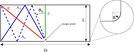
Figure 1: (Color online) The rectangular billiard, with dimension $L\times D$, has four rounded corners (with radius $R$, see magnification of just one border). The escape point with aperture $a$ lies exactly in the middle of the billiard. Initial angle $\theta_{0}$ and, schematically, the shortest escape trajectories ($P,E,A_{2}$ and $A_{4}$) are shown. In all simulations we use $L=4$ and $D=10$.

For $R/L=0$ some orbits ($P,E,A_{2},A_{4}$) are shown schematically in Fig. 1, whose inital angles are $\theta_{0}^{(n)}=\arctan{\left[\frac{D}{2nL}\right]}$. For the closed billiard these are periodic orbits with period $q=2^{n}$ ($n=1,2,3,\ldots$).

The closed rectangular billiard is integrable in the absence of corner effects ($R=0$). All Lyapunov exponents are zero and the dynamics can be described in terms of invariant tori. Such regular dynamics is shown in the the phase-space of Fig. 2(a), where the collision angle $\theta$ is plotted as a function of horizontal coordinate $x$. Tori with irrational winding numbers are the straight lines parallel to the $x$-axis. Tori with rational winding numbers are periodic orbits and are the marginally unstable periodic orbits (MUPOs) from this problem. When opening up the billiard, ICs which start on an irrational torus will certainly escape the billiard after some time, but trajectories which start exactly on a rational tori will never leave the billiard, except for those ICs which match the opening channel.

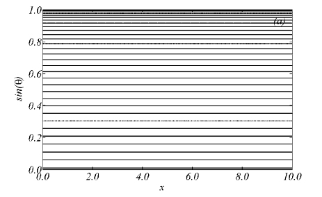
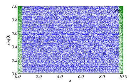
Figure 2: (Color online) Phase-space dynamics for (a) $R=0$ and (b) $R/L=0.1$ (one IC): Green (light gray) points occur when the trajectory collides with the rounded corner and defines the scattering region (SR) or chaotic region. Blue (dark gray) points occur when the trajectory collides with the vertical and horizontal parallel walls.

Figure 2(b) shows the phase-space dynamics when $R/L=0.1$ starting from one IC $\theta_{0}=0.86$. Blue points are related to points along the trajectory which collide with vertical and horizontal parallel straight walls, while green points are those which collide with the rounded corner. What happens is that the trajectory starts on an irrational torus, travels along this torus (blue horizontal lines) until it collides with one of the rounded corners (green points) and is scattered there to a new torus. It travels on this new tori until it is scattered again to another tori. This procedure repeats itself until the whole phase space is filled. This is exactly what happens in Fig. 2(b), obtained using just one initial condition. The rounded corner is called scattering region (SR) and generates the chaotic dynamics. Although there are no regular islands in phase space, sticky motion occurs due to the existence of MUPOS, as explained in details in Custodio and Beims (2011). For some of the horizontal lines in Fig.2(b), there are some regions without points. These are trajectories very close to the periodic orbits (closed billiard case) shown in Fig. 1, and before they can visit all the points on the horizontal line, they are scattered by the SR to another horizontal line.

In order to analyze the effect of rounded corners on the emission angles dynamics we start simulations at times $t=0$ from the open channel, uniformly distributed from $x_{0}=D/2$, with an initial angle $\theta_{0}$ towards the inner part of the billiard with velocity $|\vec{v}|=1$. Elastic collisions are assumed at the billiard boundaries and at the rounded corners of the open channel. For each of the $10^{5}$ IC distributed uniformly in the interval $1.00\times 10^{-2}\lesssim\theta_{0}\lesssim 1.57$ we wait until the particle leaves the billiard and record $\theta_{f}$. In all cases $a=0.4$.

The complex dynamics generated by the rounded corners becomes apparent when the escape angles $\theta_{f}$ are plotted as function of the initial incoming angle $\theta_{0}$ and for different ratios $R/L$. This is shown in Fig. 3 which was obtained by using $10^{3}\times 10^{3}$ points in the interval $2.0\times 10^{-3}\leq R/L\leq 0.35$ [$-6.0\leq\log{(R/L)}\leq-1.0$].

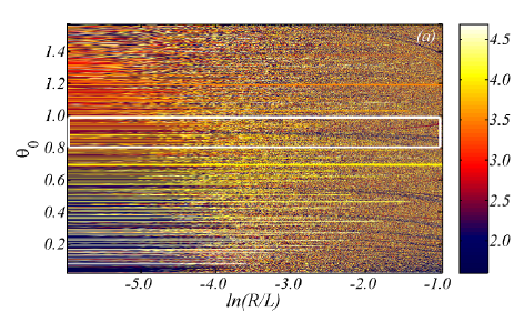
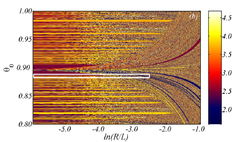
Figure 3: (Color online) (a) Escape angle as a function of $\log{(R/L)}$ and $\theta_{0}$, (b) and (c) are magnifications.

Figure 3(a) shows $\theta_{f}$ as a function of $\log{(R/L)}$ and $\theta_{0}$. Each color is related to one emission angle $\theta_{f}$ (see the colorbar on the right: dark blue $\to$ red $\to$ yellow $\to$ white in the colorscale and dark gray to white in the grayscale). These emission angles vary between $\theta_{f}\sim 1.4$ (almost horizontally to the left) and $\theta_{f}\sim 4.5$ (almost horizontally to the right). It is possible to observe [better seen in the magnifications, Figs. 3(b) and (c)] that there are always intervals of ICs which leave to the same $\theta_{f}$ (same color). As $R/L$ increases, they appear as horizontal lines with the same color, and are called here as “isoemissions stripes”. As $R/L$ increases more and more, some isoemissions stripes survive while others are destroyed or mixed. Examples of such stripes are seen in Fig. 3(a) around $\theta_{0}\sim 0.7$ (yellow), in Fig. 3(b) around $\theta_{0}\sim 0.9$ (brown), among many others. In general, the emission angles show a very rich dynamics due to the increasing rounded corners, alternating between all possible colors.

Figure 3(b) shows a magnification from Fig. 3(a). The magnification is taken around the isoemissions stripe related to the trajectory $E$ ($\theta_{0}\sim 0.89$) shown in Fig. 1. We observe that a new stripe emerges symmetrically from the middle of the isoemissions stripe. Different from the isoemissions stripe, inside this new stripe inumerous distinct escape angles (colors) appear. This new stripe is called “chaotic stripe” for reasons which become clear later. The width of the chaotic stripe increases linearly with $R/L$. Outside the isoemissions stripe a large amount of smaller stripes with distinct angles can be observed. In order to show this in more details and to explain the physics involved in the emission angles, we discuss next a magnification of Fig. 3(b) (see white box). This is shown in Fig. 3(c), where a sequence of isoemissions (yellow and purple) and chaotic (all colors) stripes appear. ICs which start inside the chaotic stripes collide, at least once, with the rounded corner so that distinct emission angles can be observed. Different from what is observed from border effects Custodio and Beims (2011), here the sequence of isoemissions stripes in Fig. 3(b), and the corresponding multicolor chaotic stripes from Fig. 3(c), are not born at the boundary between the purple (black) and orange (white) escape angles at $R/L\sim 0$. The rich and complex dynamics is always generated from ICs starting inside the chaotic stripes, so that a large amount of different colors in the emission angles appears, showing that tiny changes or errors in the initial angle may drastically change the emission angle. The location of the chaotic stripes itself is not self-similar, but inside the chaotic stripes the self-similar structure is evident. Chaotic stripes which emerge at different initial angles at $R/L\sim 0.0$ increase their width with $R/L$ and start to overlap for $R/L\sim 0.05$, where the dynamics of strongly sensitive to initial angles $\theta_{0}$. The width of the stripes increase with $R/L$ and allows us to characterize the different domains of the dynamics.

The dynamics generated by starting with IC inside the chaotic stripes is the consequence of trajectories which collide with the rounded corner and the chaotic motion appears. The collision with the rounded border was checked numerically (not shown) and the chaotic motion has to be demonstrated. To do this we use the ETs statistic defined Altmann et al. (2005) by $Q(\tau)=\lim_{N\to\infty}\frac{N_{\tau}}{N},$ where $N$ is the total number of recurrences and $N_{\tau}$ is the number of recurrences with time $T\geq\tau$. The time $T$ is recorded when the trajectory returns to the recurrence region, which is the open channel. In our model, when a trajectory returns to the open channel it leaves the billiard. Thus, since we have an open system, the number of recurrences is counted over distinct ICs. In chaotic hyperbolic systems the ETs statistic decays exponentially while systems with stickiness it decays as a power law $Q(\tau)\propto\tau^{-\gamma_{esc}}$ with $\gamma_{esc}>1.0$ being the scaling exponent. Usually it is assumed to have stickiness when a power-law decay with $\gamma_{esc}>1.0$ is observed for two decades in time. Power-law decays with $\gamma_{esc}=1.0$ Bauer and Bertsch (1990); Custodio and Beims (2011) appear in integrable systems, which is the case of our model when $R/L=0.0$.

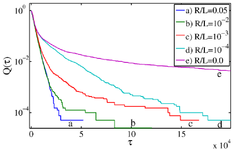
Figure 4: (Color online) Semi-log plot of $Q(\tau)$ for distinct values of $R/L$. Each curve was obtained using $2.0\times 10^{4}$ ICs.

Figure 4 displays in a semi-log plot the quantity $Q(\tau)$ obtained using different values of the ratio $R/L=0.0,1.0\times 10^{-4},1.0\times 10^{-3},1.0\times 10^{-2},5.0\times 10^{-2}$, where $L$ is kept fixed. ICs are $1.00\times 10^{-5}\leq\theta_{0}\leq 1.57$ and $-1.00\times 10^{-5}\leq\theta_{0}\leq-1.57$. Straight lines in this plot are exponential decays. For the integrable case $R/L=0.0$ (curve $e$) a power law decays occurs with $\gamma_{esc}\sim 1.0$. Trajectories close to the periodic orbits inside the rectangle generate the power-law decay with $\gamma_{esc}=1.0$. Small corner effects, $R/L=1.0\times 10^{-4}\to 1.0\times 10^{-3}$ (see curves $d\to c$), change the qualitative behavior of $Q(\tau)$ so that regular trajectories close to MUPOs generate, for small period of times, a power-law decay with $1.0<\gamma_{esc}<2.0$. For a detailed discussion of a similar behavior we refer the reader to Custodio and Beims (2011). However, for $R/L=1.0\times 10^{-2}[\log(R/L)=-4.6],5.0\times 10^{-2}[\log(R/L)=-3.0]$ (curves $b,a$), which correspond to values from Fig. 3(c), a straight line decay is observed, characterizing the transition to an almost totally chaotic motion when stripes overlap.

Summarizing results for the billiard model, we showed that specific intervals of ICs, called chaotic stripes, which increase linearly with the nonlinear parameter, generate chaotic trajectories. Outside these stripes we have the isoemissions stripes, for which the ICs generate a regular motion. For smaller values of the parameter, we have a mixture of regular and chaotic motion, i.e. a mixture of a large amount of isoemissions stripes and few chaotic stripes, and the system is weakly chaotic. Only when the nonlinear parameter increases, so that all chaotic stripes overlap, the whole system becomes chaotic.

III Stripes in Coupled maps

At next we analyze the IC dependence of the dynamics of $4$ particles globally coupled on a discrete lattice. It has a $8$-dimensional phase space and particles are coupled on a unit circle, where the state of each particle is defined by its position $2\pi x^{(i)}$ and its conjugate momentum $p^{(i)}$. The dynamics on the lattice obeys T.Konishi and K.Kaneko (1990)

$$\left\{\begin{array}[]{ll}p_{t+1}^{(i)}=p_{t}^{(i)}+\frac{K}{2\pi\sqrt{3}}\sum_{j=1,j\not=i}^{N=4}\sin[2\pi(x_{t}^{(j)}-x_{t}^{(i)})],\\ \\ x_{t+1}^{(i)}=x_{t}^{(i)}+p_{t+1}^{(i)},\end{array}\right.$$ (4)

where mod $1$ must be taken in the variables $p^{(i)},x^{(i)}$, and $i=1,\ldots,N=4$. For $K>0$ the interaction between two particles $i$ and $j$ is attractive T.Konishi and K.Kaneko (1992). For this coupling the total momentum $P_{T}=\sum_{j=1}^{N=4}p^{j}_{t}$ is preserved. This model has $8$ Lyapunov exponents which come in pairs. The reasons for using such a model are: (i) these are coupled standard maps, thus their properties should be valid for a large class of physical systems; (ii) the phase space dynamics is $8$, thus it can be used to show that, in case results are similar to those from Section II, they are valid for higher dimensions and connect the chaotic stripes to the Arnold web.

An interesting way to describe the complicated dynamics dependence on ICs is shown in the plot $K\times p_{0}^{(2)}$ from Fig. 5. In colors is plotted the largest FTLE after $10^{4}$ iterations. Initial conditions are chosen on the invariant structure $P_{T}=0.0$ and $X_{CM}=0.0$. This plot shows, as a function of $K$, those ICs $p_{0}^{(2)}$ which generate the regular, mixed or chaotic motion. While black colors describe initial conditions with generate a regular motion, with zero FTLEs, cyan, red to yellow colors are obtained from ICs which generate increasing positive FTLEs.

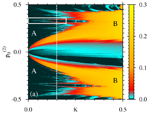
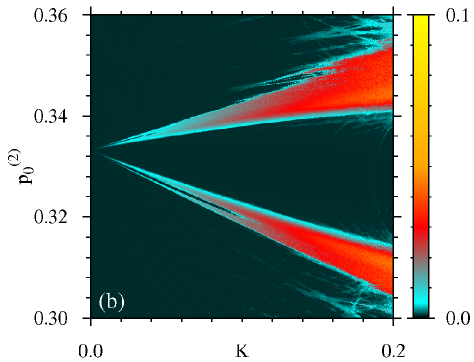
Figure 5: (Color online) Grid of $1000\times 1000$ points with the FTLEs as a function of $K\times p_{0}^{(2)}$.

A rich variety of structures is observed. Essentially two distinct larger regions of motions are observed and demarked in the plot as: (A) where FTLEs are smaller and (B) where FTLEs are larger. In between the FTLEs mix themselves along complicated and apparently fractal structures. For $K\to 0$ FTLEs also go to zero inside region (A). However there are some stripes, which emanate from $K\sim 0$ for which FTLEs are larger. Two larger stripes are born close to $p_{0}^{(2)}\sim 0.0$ and growth symmetrically around this point as $K$ increases. ICs which start inside the stripes generate chaotic trajectories. Thus these stripes correspond to the chaotic stripes found in the billiard case in Sec. II. Along the line $p_{0}^{(2)}\sim 0.0$ the dynamics is almost regular for $K<1$, becoming chaotic for larger values of $K$. This picture shows us clearly that for the same $K$ value, different ICs (in this case $p_{0}^{(2)}$) have distinct FTLEs. Zero FTLEs are related to regular trajectories, larger FTLEs are related to chaotic trajectories and intermediate FTLEs are related to chaotic trajectories which touched, for a finite time, the regular structures from the high-dimensional phase space. Such regular structures can be global invariants (as $P_{T}$) or local, or collective ordered states which live in the high-dimensional phase space. As trajectories itinerate between ordered and random states, the regular structures affect locally the FTLEs inducing sticky motion, so that the corresponding FTLEs decrease. Thus each point in the mixed plot from Fig. 5(a) with and intermediate FTLE for a fixed $K$ value, is necessarily related to a trajectory which suffers sticky motion. Figure 5(b) is a magnification of Fig. 5(a) and shows similar stripes structures observed in the billiard case. As the nonlinear parameter $K$ increases, the width of the chaotic stripes increase and they start to overlap, generating the totally chaotic motion, but only for higher $K$ values (not shown).

It is very interesting to observed that the chaotic stripes define the channels of chaotic trajectories which form the Arnold web Zaslavsky (2008) which allows the Arnold diffusion to occur in higher-dimensional systems. This can be better understood when the FTLEs are plotted in the phase space projection $p_{0}^{(1)}\times p_{0}^{(2)}$, shown in Fig. 6 for $K=0.15$ [see dashed line in Fig.5(a)].

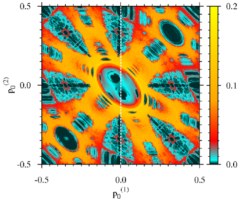
Figure 6: (Color online) FTLEs in the phase space projection $p_{0}^{(1)}\times p_{0}^{(2)}$ for $K=0.15$ [see white dashed line in Fig. 5(a)].

Black points are related to close to zero FTLEs, while purple, red to yellow points are related to increasing FTLEs. This picture is similar to the one shown in K.Kaneko and T.Konishi (1994) (but in black and white), and presents a form called as “onion”. In fact, this plot shows an Arnold web, or stochastic web, where points with larger FTLEs are the chaotic channels inside which the Arnold diffusion occurs. The FTLEs along the line $p_{0}^{(1)}=0.0$ in Fig. 6 are exactly the FTLEs along the white dashed line in Fig. 5(a). In other words, ICs for $K=0.15$ [white dashed line in Fig. 5(a)], inside the chaotic stripes, are those which generate trajectories with positive FTLEs and correspond exactly to the positive FTLEs from Fig. 6 for $p_{0}^{(1)}=0.0$ (see also white dashed line). Thus the chaotic stripes define the width of the chaotic channels, for a given $K$, inside which Arnold diffusion occurs as time increases. Summarizing, the chaotic stripes in Fig. 5 show directly the intervals of ICs where the chaotic channels are located and how the Arnold web changes with $K$.

IV Conclusions

Chaotic stripes are shown to generate weakly chaotic dynamics for two distinct Hamiltonians systems, namely an open rectangular billiard with rounded corners and $4$ globally coupled particles on a discrete lattice. The width of the stripes increase with the nonlinear parameter and allow us to characterize the different domains of the dynamics. For the billiard case the stripes define injection angles which generate an chaotic dynamics inside the billiard and an uncertainty about ejection angles. For small values of the nonlinear parameter but higher-dimensional systems, the stripes are the chaotic channels in the Arnold web inside which the Arnold diffusion occurs Zaslavsky (2008). From this perspective we can define the chaotic stripes as Arnold stripes. We also observed such stripes for Hamiltonian systems with higher values of $N>4$ and other couplings (not shown here). This suggests that weak chaos in Hamiltonian systems always emerges inside stripes of particular ICs. This is of relevance since in such systems finite time distributions, independently of the considered physical quantity, are not Gaussians anymore and decay rates of recurrences and time correlations are difficult to obtain Artuso and Manchein (2009); Manchein et al. (2011). For higher values of the nonlinear parameters a totally chaotic motion is observed due to the overlap of Arnold stripes.