Predictions of just-enough inflation

Abstract

We find the best-fit cosmological parameters for a scenario of inflation with only the sufficient amount of accelerated expansion for the $\lambda\phi^{4}$ potential. While for the simplest scenario of chaotic inflation all observable primordial fluctuations cross the Hubble horizon during the slow-roll epoch, for the scenario of just-enough inflation the slow-roll conditions are violated at the largest length scales. Performing a numerical mode-by-mode integration for the perturbations on the largest scales and comparing the predicted anisotropies of the cosmic microwave background to results from the WMAP 7-yr data analysis, we find the initial conditions in agreement with current cosmological data. In contrast to the simplest chaotic model for the quartic potential, the just-enough inflation scenario is not ruled out. Although this scenario naturally gives rise to a modification of the first multipoles, for a quartic potential it cannot explain the lack of power at the largest angular scales.

I introduction

Early Universe Inflation is considered the physical process behind the generation of perturbations that produce the large-scale structures observed in the Universe today as well as the mechanism that solves the main problems of the standard cosmological scenario. As a proposal still lacking a fundamental theory from which it could emerge, there is a variety of scenarios which achieve the fundamental aim of inflation in different manners.

Current observational results K10 start to constrain the application of the chaotic inflation scenario linde83 for single-field inflation models. A variation of chaotic inflation contemplates having only a small amount of accelerated expansion, just enough to solve the causality and flatness problems of the hot big bang model. In this scenario, the initial fast-roll dynamics has observational consequences at the larges scales, the physics of smaller scales is determined by the subsequent era of slow-roll inflation. This setup has been considered to explain the lack of power observed in the lower multipoles of the CMB cpkl ; vsb . Other works have analyzed initial conditions for this scenario in the context of a preinflationary radiation-dominated Universe ws ; pk and initial conditions for the perturbations different from a Bunch–Davies vacuum ddr .

In previous works rs ; sr , we proposed a modification of the chaotic inflation scenario also with a limited amount of exponential expansion which is in accordance with recent observations. Our motivation considered the fact that some theories of fundamental physics, including the standard model of particle physics, stop being valid above a certain energy scale. In those cases, applying chaotic initial conditions would imply a complex potential and a decaying inflaton field. By considering an amount of inflation of no more than 50 to 60 $e$-foldings of exponential expansion this situation can be avoided. As a consequence, the Universe starts out in a kinetic-energy-dominated stage with an inflaton potential which is many orders of magnitude smaller than the Planck scale to the fourth, but is real and well defined. This situation initially causes a violation of the slow-roll conditions at the moment of horizon crossing when perturbations are evaluated, but the Universe rapidly joins the attractor (slow-roll) regime.

Regardless of this initial violation of slow-roll, we based our previous results on the slow-roll expansion. The aim of this work is to formalize the implementation of this scenario by integrating the mode equations for inflationary perturbations in a way consistent with its initial conditions and find those values that best characterize this scenario in accordance with current data by means of a Monte Carlo integration. Here we limit ourselves to the $\lambda\phi^{4}$ potential only, once the the mode integration is carried out correctly, one can consider the application of this scenario to arbitrary potentials.

II mode integration

For the purposes of our work, we need to integrate the mode equations for the cosmological perturbations for scalar and tensor modes. The fact that this scenario of inflation naturally induces a violation of scale invariance on observable scales, means that we cannot approximate the power spectra and higher-order observables by a power law, as doing so would rely on the validity of the slow-roll approximation.

Our intention is to obtain the initial conditions that predict values for the power-spectra and spectral indices which are in accordance with current data. We therefore need to integrate the mode equations numerically and insert this new information into the CAMB code lcl to supply it with the spectra and then into the COSMOMC code lb . All relevant information on how this is done is provided in the next subsections.

II.1 Equations of motion : background

As a first approximation, in this work we still assume homogeneity, isotropy and flatness from the very beginning of inflation. The equations of motion for the background are then

$$\scriptstyle\displaystyle H^{2} \scriptstyle\displaystyle= \scriptstyle\displaystyle\frac{1}{3M_{p}^{2}}\left(\frac{\dot{\phi}^{2}}{2}+V\right),$$ (1)

$$\scriptstyle\displaystyle\ddot{\phi}+3H\dot{\phi}+V^{\prime} \scriptstyle\displaystyle= \scriptstyle\displaystyle 0;$$

a prime denotes a derivative with respect to the scalar field $\phi$, a dot means derivative with respect to cosmic time, $H$ is the Hubble rate, whereas $V$ represents the inflaton potential. In this case, we adopt the notation $V=\frac{\lambda\phi^{4}}{24}$ and $M_{p}\equiv m_{p}/\sqrt{8\pi}\approx 2.4\times 10^{18}$ GeV is the reduced Planck mass.

We perform all integrations with respect to the number of $e$-foldings $N$, which means for the differential equations that

$$\scriptstyle\displaystyle\frac{dH}{dN} \scriptstyle\displaystyle= \scriptstyle\displaystyle\frac{V}{M_{p}^{2}H}-3H$$ (2)

$$\scriptstyle\displaystyle\frac{d\phi}{dN} \scriptstyle\displaystyle= \scriptstyle\displaystyle-\sqrt{6M_{p}^{2}-\frac{2V}{H^{2}}}$$

Our convention is as follows: $\dot{\phi}<0\Rightarrow H^{\prime}>0$, then the inflaton roll downs the potential from right to left and $H\equiv dN/dt$ with $t$ cosmic time, therefore $dN>0$ as $dt>0$.

In what follows, we make use of the horizon flow functions $\epsilon_{n}$ stg , developed as a generalization of the slow-roll parameters and defined as

$$\scriptstyle\displaystyle\epsilon_{0}\equiv\frac{H_{i}}{H},\quad\epsilon_{m+1}\equiv\frac{1}{\epsilon_{m}}\frac{d\epsilon_{m}}{dN},\,\,m\geq 0.$$ (3)

$H_{i}$ refers to the initial Hubble rate (at $N=0$). In the case of single-field inflation models, the function $\epsilon_{1}$ represents the ratio of the kinetic energy to the total energy density of the field,

$$\epsilon_{1}=3{\frac{\frac{1}{2}\dot{\phi}^{2}}{\frac{1}{2}\dot{\phi}^{2}+V}}.$$ (4)

In the scenario of inflation being considered, the initial value of the potential is limited to be much less than the Planck mass such that : $V_{i}\sim M^{4}\ll M_{p}^{4}$, where $M$ represents a scale that bounds the validity of the theory under consideration. This means that the evolution of the system starts in a stage of kinetic energy domination, which later naturally leads to one of potential energy domination shortly after inflation starts. Within this picture, it is valid to consider an initial condition for the function $\epsilon_{1,i}$ corresponding to a value bigger than 1, linde , but for a stage of kinetic energy domination, an initial condition close to 3 comes out more naturally from Eq. (4), as $\dot{\phi}^{2}_{i}\sim M_{p}^{4}\gg V_{i}$.

II.2 Equations of motion : perturbations

In order to calculate the power spectra, we need to integrate the equations that describe the evolution for inflationary perturbations. We follow the notation and conventions of muk and write the equations for scalar and tensor modes in the following manner:

$$\scriptstyle\displaystyle\frac{d^{2}u_{k}^{S}}{d\tau^{2}}+\left(k^{2}-\frac{1}{z}\frac{d^{2}z}{d\tau^{2}}\right)u_{k}^{S}=0\quad{\rm scalars,}$$ (5)

$$\scriptstyle\displaystyle\frac{d^{2}u_{k}^{T}}{d\tau^{2}}+\left(k^{2}-\frac{1}{a}\frac{d^{2}a}{d\tau^{2}}\right)u_{k}^{T}=0\quad{\rm tensors,}$$

where $u$ is defined in muk as a gauge-invariant combination of field and metric perturbations. The comoving wave number $k$ is introduced to calculate the power spectra through a Fourier expansion. The quantity $z$ is defined as $z\equiv a\dot{\phi}/H$, where $a$ is the scale factor and $\tau$ is conformal time defined as $d\tau=dt/a(t)$.

As mentioned before, we are integrating all quantities with respect to the number of $e$-foldings $N$, in consequence, the perturbation equations are rewritten and integrated as

$$\scriptstyle\displaystyle\frac{d^{2}u_{k}^{S}}{dN^{2}}+(1-\epsilon_{1})\frac{du_{k}^{S}}{dN}+\left[\left(\frac{k}{aH}\right)^{2}-f_{S}(\epsilon_{1},\epsilon_{2},\epsilon_{3})\right]u_{k}^{S} \scriptstyle\displaystyle= \scriptstyle\displaystyle 0,$$ (6)

$$\scriptstyle\displaystyle\frac{d^{2}u_{k}^{T}}{dN^{2}}+(1-\epsilon_{1})\frac{du_{k}^{T}}{dN}+\left[\left(\frac{k}{aH}\right)^{2}-f_{T}(\epsilon_{1})\right]u_{k}^{T} \scriptstyle\displaystyle= \scriptstyle\displaystyle 0,$$

where $f_{S}(\epsilon_{1},\epsilon_{2},\epsilon_{3})=2-\epsilon_{1}+\frac{3}{2}\epsilon_{2}-\frac{1}{2}\epsilon_{1}\epsilon_{2}+\frac{1}{2}\epsilon_{2}\epsilon_{3}+\frac{1}{4}\epsilon_{2}^{2}$ and $f_{T}(\epsilon_{1})=2-\epsilon_{1}$, writing $\frac{1}{z}\frac{d^{2}z}{d\tau^{2}}$ and $\frac{1}{a}\frac{d^{2}a}{d\tau^{2}}$ in Eq. (5) in terms of the horizon flow functions (3).

When perturbations are generated inside the horizon, in the region where $k/aH\rightarrow\infty$, the modes approach plane waves of the form muk

$$u_{k}(\tau)\rightarrow\frac{1}{\sqrt{2k}}e^{-ik\tau},$$ (7)

whereas in the opposite limit, when they are outside the horizon $\frac{k}{aH}\rightarrow 0$, the solution is $u_{k}\rightarrow z$.

In our case, in order to set the initial conditions for equations (6), we need to consider that the system is not in the slow-roll regime and we are actually starting the mode integration from the very beginning of inflation. At this point, we make another approximation which needs to be improved; we set the initial conditions for the perturbations assuming the Bunch-Davies vacuum Eq. (7). This clearly needs to be reconsidered as it should not be necessarily the case that from the very beginning of inflation the part of the Universe on which inflation starts corresponds to the vacuum state of the field when there is kinetic energy domination. Our initial conditions are therefore different from those adopted in cpkl for a similar situation.

We also need to establish a way to determine the value of the first mode to be integrated, the other modes will be generated from this value. We follow the discussion of Ref. (muk ), section 11 in which a consistent initial condition keeps the terms $\left(k^{2}-\frac{1}{z}\frac{d^{2}z}{d\tau^{2}}\right)$, and $\left(k^{2}-\frac{1}{a}\frac{d^{2}a}{d\tau^{2}}\right)$ in Eq. (5) positive at the beginning of inflation. Therefore the minimum value of $k$ that we choose is given by the maximum of the initial values between the terms $\left|\frac{1}{z}\frac{d^{2}z}{d\tau^{2}}\right|$ and $\left|\frac{1}{a}\frac{d^{2}a}{d\tau^{2}}\right|$ which are determined by the background initial conditions given by this scenario.

The initial conditions we use for the scalar and tensor perturbations for each mode $k$ in terms of $N$ are

scalars	tensors
$u_{k}^{S}=\frac{1}{\sqrt{2k}}e^{-ik\tau}$,	$u_{k}^{T}=\frac{1}{\sqrt{k}}e^{-ik\tau}$,
$\frac{du_{k}^{S}}{dN}=-u_{k}^{S}\left(\frac{k}{a_{i}H_{i}}\right)$,	$\frac{du_{k}^{T}}{dN}=-u_{k}^{T}\left(\frac{k}{a_{i}H_{i}}\right)$,

The expressions we use to calculate the power spectra are given by llms

$$\scriptstyle\displaystyle P_{R} \scriptstyle\displaystyle= \scriptstyle\displaystyle\frac{k^{3}}{4\pi^{2}M_{p}^{2}}\left|\frac{u_{k}^{S}}{z_{S}}\right|^{2},$$ (8)

$$\scriptstyle\displaystyle P_{T} \scriptstyle\displaystyle= \scriptstyle\displaystyle\frac{2k^{3}}{\pi^{2}M_{p}^{2}}\left|\frac{u_{k}^{T}}{z_{T}}\right|^{2},$$

with $z_{S}=a\sqrt{\epsilon_{1}},\,\,\,z_{T}=a$. Once the first mode $k_{min}$ to be integrated is determined as indicated above, we consider the mode $k_{max}=10^{5}k_{min}$ as the biggest value of interest for the mode integration. From them we generate 200 equally spaced modes to perform the integration of equations (6) along with the background equations (2) for each of the modes.

II.2.1 Integration Method

We followed the structure of the code in Ref. lsv with the difference that we do not start the integration at the pivot point $k=aH$ but before inflation starts and do not Taylor expand any of the quantities being integrated as we are working with a specific potential. The structure of the mode integration as performed in the code was done in the following manner: given an initial value of $\epsilon_{1}$ above 1, one has to find the place where inflation starts and reset the number of $e$-foldings to 0 to discard the expansion that is noninflationary. At this moment one determines the value of the first and last modes that will be integrated with the perturbation equations as described in the previous paragraph. Then, the background equations are integrated until the end of inflation to find the values of the potential, Hubble rate, and quantities that will be used to convert each of the modes, whose wave numbers are given in GeV to units of Mpc^-1 as needed for the CAMB code. We assume sudden reheating to establish this correspondence :

$$k_{Mpc^{-1}}=\frac{c}{h}k_{min}\frac{T_{\nu 0}}{T_{end}}\exp^{-\Delta N}H_{*}(1.5\times 10^{38}),$$ (9)

where $c$ is the speed of light in km/s, $h$ is the Hubble constant which we take equal to 70, $k_{min}$ corresponds to the minimum scale in the CAMB code in units of Mpc^-1, $T_{\nu}$ is the temperature of neutrinos today, $T_{end}$ the temperature after reheating, $\Delta N=N_{end}-N_{*}$, is the number of $e$-foldings between horizon crossing $N_{*}$ and the end of inflation $N_{end}$, $H_{*}$, the value of the Hubble rate at horizon crossing and the factor $1.5\times 10^{38}$ is used to convert from GeV to Mpc^-1.

In the code, the perturbation equations and the background equations are integrated beyond horizon crossing until decaying and growing modes of scalars and tensors have evolved completely and the amplitudes are frozen-in. This happens for tensors at $k\approx\frac{1}{14}aH$, a bit later than for scalars, since the term $\frac{1}{a}\frac{da^{2}}{d\tau^{2}}$ in Eq. (5) is bigger than the term $\frac{1}{z}\frac{d^{2}z}{dz^{2}}$ at the beginning of inflation. Consequently we integrate both spectra up to this value. In order to optimize the computational time, we only integrate the perturbation equations until the Universe joins the slow-roll regime and the amplitudes of both spectra have a difference of less than $10^{-2}$ with respect to the corresponding slow-roll expressions. Then we only take the later as input into the CAMB code. At the same time, the system of background equations is integrated to find the moment of horizon crossing at $k=aH$ and use those values for the conversion of units for the scales.

III monte carlo integration

One of our main purposes in this work, is to find the best-fit cosmological parameters for the scenario of inflation mentioned in the Introduction by considering initial conditions for the background and perturbations as described at the end of subsection II.1 and II.2. Since this scenario produces primordial spectra that differ from the usual power-law parameterization, we wrote a module that can be used to provide the CAMB code with the information generated by the mode integration and then be introduced, into the COSMOMC code. In our case, the information needed to do the mode integration are the initial values of the first horizon flow function $\epsilon_{1,i}$, the initial value of the scalar field $\phi_{i}$, and when varied, a range of values for the coefficient $\lambda$ of the potential. If this parameter is fixed, then we consider a value of $10^{-12}$ to get the amplitude of scalar perturbations correct.

We reused the parameters in the CAMB and COSMOMC codes which are no longer needed to parameterize the primordial power spectra and characterize other inflationary observables since we determine them directly from the mode integration .

We use WMAP7 data K10 only to perform the MCMC analysis. We vary the following parameters : the physical densities of baryons, $\Omega_{b}h^{2}$, and dark matter, $\Omega_{DM}h^{2}$, and the reionization optical depth $\tau$ along with the three parameters mentioned before ($\epsilon_{1,i},\phi_{i},\lambda$). We do not vary the Sunyaev-Zel’dovich template and fix its value to 1. From there the code also varies the ratio of the sound horizon to the angular diameter distance $\theta$. The equation of state of dark energy is not varied and is set to $w=-1$. The model, as implemented in the COSMOMC package delivers the posterior distributions of 13 cosmological parameters, but at most 7 of them are independent. That is, one extra parameter compared to a $\Lambda$ Cold Dark Matter scenario of cosmology implemented without varying the Sunyaev-Zel’dovich template and without including tensor modes, with the following parameters : $\Omega_{b}h^{2}$, $\Omega_{DM}h^{2}$, $\theta$, $\tau$, $n_{s}$ and $A_{s}$. We therefore apply the Akaike information criterion to our results to measure the difference in goodness of fit. This is presented below when we discuss our results.

III.1 Initial conditions

We have mentioned that a natural initial condition for the scenario here considered corresponds to the first horizon flow function being close to 3 which determines the initial value for the Hubble rate through the equation

$$H_{i}=\frac{1}{\sqrt{3-\epsilon_{1,i}}}\sqrt{\frac{Vi}{M_{p}^{2}}}.$$ (10)

The initial value of the scalar field determines the initial value of the potential. From the slow-roll approximation, one can give an estimate of the interval where the initial value of the scalar field must vary in order to give the minimum amount of inflation required to solve the horizon and flatness problems of the standard cosmological scenario. Here we consider an interval for the field given by $\phi_{i}/M_{p}=[20,25]$ and let the data decide how to adjust the interval, after each run.

The code takes into account the fact that, when looking at different regions in parameter space for $\epsilon_{1,i}$ and $\phi_{i}/M_{p}$, there might be a numerical issue concerning the way in which the initial value of $k_{*}$ is chosen; sometimes it could be, that the ratio $k/{aH}$ is too close to 1 already from the very beginning of inflation. If one is asking the code to determine the moment of horizon crossing and does the mode integration as long as this value is less than 1, the numerical accuracy might not be enough to avoid the evaluation being omitted. The reason is that we are choosing $k_{min}=\left(\frac{1}{a}\frac{d^{2}a}{d\tau^{2}}\right)^{1/2}$ which is bigger than the corresponding term for the scalars as we want to be assured that both terms $\left(k^{2}-\frac{1}{a}\frac{da^{2}}{d\tau^{2}}\right)$ and $\left(k^{2}-\frac{1}{z}\frac{d^{2}z}{dz^{2}}\right)$ in Eq. (5) are positive. If $\epsilon_{1,i}>1$, $k_{min}$ is chosen at the moment when inflation has just started and $\epsilon_{1}$ has become just one time step smaller than 1 and $k_{min}^{2}\approx a^{2}H^{2}$. In a situation when the initial $\epsilon_{1}\ll 1$, and the initial $k$ is still chosen in the way we do for $\epsilon_{1}>1$, then $k_{min}/aH\simeq\sqrt{2}$ which is also very close to 1. This problem does not appear in the standard way in which the mode integration is done, because the value of $k$ is taken within the range reached by observations and the initial value of $\epsilon_{1}$ is considered to be in the slow-roll regime, then they are not correlated in the way ours are.

III.2 Regions explored for the initial conditions

From Eq. (10) one can observe that $\epsilon_{1}<3$. Therefore an initial value of $\epsilon_{1}$ could be in principle arbitrarily close to 3 from below making the initial Hubble rate approach the value of $M_{p}$ as long as 3 is avoided and the numerical accuracy is enough to distinguish them. Apart from this, we also explore other possibilities in the Monte Carlo integration. We consider values of $\epsilon_{1,i}$ as low as 2 with the consequence that one has to reduce the interval on which the initial value of the field can vary so that the potential studied in this case can agree with the data. If $\epsilon_{1,i}\ll 3$, the initial Hubble rate is some orders of magnitude below $M_{p}$ because the potential in this scenario is approximately 8 orders of magnitude smaller than $M_{P}^{4}$.

We also explored the interval [0.001,2.999] for the initial value of $\epsilon_{1}$. We switched off the lensing for this run, as it turned out that such a broad prior on $\epsilon_{i}$ is computationally intense, as is the lensing itself. Our final conclusions are not based on this run, but it provides a nice consistency check.

IV results

Table 1: Summary of main results for Monte Carlo integration showing the allowed ranges for the initial values of $\epsilon_{1}$, the field and the quartic coupling $\lambda$. For all cases $20\%$ of rows have been excluded. Values of $\epsilon_{1,i}$ and $\phi_{i}/M_{P}$ outside the indicated intervals are disfavored by the data. In all cases the tensor modes have been included.

	$\epsilon_{1,i}$	$\phi_{i}/M_{p}$	$\lambda$	lensing	ind. samples	burn in steps	R-1
1	[2.85,2.999]	[23.55,25.4]	[$9.28\times 10^{-13}$,$1.26\times 10^{-12}$]	included	10 949	261	0.0017
2	[2.9,2.999]	[23.7,25]	[$9.28\times 10^{-13}$,$1.25\times 10^{-12}$]	included	20 058	188	0.0023
3	[2.6,2.999]	[22.74,25]	[$9.19\times 10^{-13}$,$1.27\times 10^{-12}$]	included	7 669	424	0.0024
4	[0.94,2.44]	[21.8,25.22]	[$9.33\times 10^{-13}$,$1.22\times 10^{-12}$]	not included	4 307	828	0.0012

We explored several regions and cases in parameter space, the most representative ones are summarized in Table LABEL:iep. For each case we had to determine a new covariance matrix since we could not use the default covariance matrix supplied with the COSMOMC program as it would overrun the settings for our initial conditions . We took flat priors on $\epsilon_{1,i}$, $\phi_{i}/M_{p}$ and $\lambda$.

The last column of Table LABEL:iep, $R-1$, corresponds to the Gelman and Rubin R statistic to asses convergence of the chains gr . These results are for 6 chains of 200,000 samples each. We use the features included in the COSMOMC code to propose a good covariance matrix but stop updating when the convergence factor R-1 is less than 0.2 to assure that the chains are strictly Markovian. The number of independent samples reported is obtained by ignoring 20$\%$ of the rows . We found that the number of independent samples is reduced considerably when the BB mode of the polarization is taken into account. As there are no useful observational constraints on the BB modes available so far, we restricted our analysis to runs with TT, TE and EE spectra only.

In Table LABEL:iep2, the mean values and standard deviations for the Markov Chains described in Table LABEL:iep are quoted. Their corresponding one-dimensional posterior distributions are shown in Figs. 1 and 2 only for the last two cases of Table LABEL:iep. In all four cases the best fit values of the three ‘noninflationary’ parameters $\Omega_{b}h^{2},\Omega_{DM}h^{2}$ and $\theta$ are in concordance with results established by other measurements (supernovae, clusters, etc.). The optical depth $\tau$ is clearly measured. The same can be said on the self-coupling $\lambda$. The initial conditions of inflation, encoded in $\epsilon_{1,i}$ and $\phi_{i}/M_{P}$ are less well constrained. We do find good fits to the data (see below), but there is also a degeneracy between these two parameters, which results in the discrepancy of the marginalized and maximized 1D posteriors in Figs. 1 to 2, see also Fig. 3 below.

The results for case 1 in Table LABEL:iep correspond to the lowest possible value of $\epsilon_{1,i}$ and lowest and highest values of $\phi_{i}/M_{p}$ in which the quartic potential is compatible with the data. A lower value of $\epsilon_{1,i}$ or wider interval for $\phi_{i}/M_{p}$ would cause all observable modes to cross the horizon during the slow-roll regime and thus would result in the exclusion of this potential. Similarly, for the cases 2 and 3 a higher value of $\phi_{i}/M_{p}$ produces the same effect; one starts to recover the slow-roll result for this potential.

Bigger initial values of the field lead to numerical problems when lensing is included. This is not the case when we turn off the lensing effect and $\epsilon_{1,i}$ and $\phi_{i}/M_{p}$ are allowed to vary from slow-roll to 2.999 and [20,26], respectively. One can observe in Fig. (2) that the posterior distribution of $\phi/M_{p}$ exhibits a maximum. For $\epsilon_{1,i}$, there is a broad region of almost equally-likely values. This also repeats in cases 1 and 3, although for a narrower interval and different initial conditions.

Table 2: Summary of main results for Monte Carlo integration. Mean values and standard deviations for examples in Table LABEL:iep.

		$\Omega_{b}h^{2}$	$\Omega_{DM}$	$\theta$	$\tau$	$\phi_{i}/M_{p}$	$\epsilon_{1,i}$	$\ln(10^{10}A_{s})$	$\Omega_{\Lambda}$	Age/Gyr	$\Omega_{m}$	$z_{re}$	$r_{10}$	$H_{0}$
1	$\mu$	0.022	0.11	1.037	0.08	24.75	2.91	-4.53	0.71	13.89	0.29	10.14	0.13	68.75
	$\sigma$	0.00032	0.0054	0.0023	0.013	0.35	0.038	0.032	0.027	0.08	0.027	1.138	0.0028	1.92
2	$\mu$	0.022	0.11	1.038	0.08	24.65	2.93	-4.53	0.71	13.87	0.29	10.1	0.13	68.63
	$\sigma$	0.00011	0.005	0.0021	0.013	0.22	0.022	0.031	0.026	0.067	0.026	1.136	0.0031	1.86
3	$\mu$	0.022	0.11	1.037	0.08	24.31	2.77	-4.53	0.71	13.89	0.29	10.13	0.13	68.75
	$\sigma$	0.00032	0.0054	0.0027	0.013	0.36	0.102	0.031	0.027	0.08	0.027	1.14	0.0029	1.92
4	$\mu$	0.022	0.11	1.037	0.08	23.43	1.69	-4.53	0.71	13.9	0.29	10.20	0.13	68.83
	$\sigma$	0.00032	0.0054	0.0022	0.013	0.39	0.43	0.032	0.027	0.08	0.027	1.15	0.0028	1.94

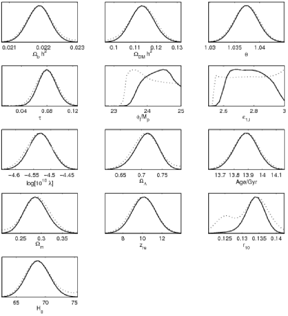
Figure 1: Posterior distributions of cosmological parameters from case 3 in Table LABEL:iep. The dotted lines represent mean likelihood of samples and solid lines marginalized probabilities.

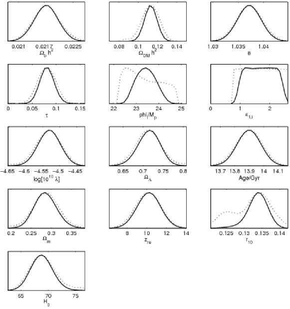
Figure 2: Posterior distributions of cosmological parameters from case 4 in Table LABEL:iep .

There are some comments concerning the shape of the distributions and the number of independent samples which are interesting. For $\epsilon_{1,i}\in[2.85,2.999]$, $\phi_{i}/M_{p}\in[23.55,25.4]$, not shown in the table, we obtain very distorted distributions and observe that this feature repeats whenever we explore regions of initial conditions for $\epsilon_{1}$ below 2.9 and do not include tensor modes. Particularly, for the interval $\epsilon_{1,i}\in[2.6,2.999]$ without tensors and $\lambda$ fixed, also not shown, the posteriors are observed to be very distorted, but this is somewhat alleviated by introducing the tensor modes and varying $\lambda$, as can be seen from Fig. 1. Reducing the initial value of $\epsilon_{1}$, below the favored values in this scenario, causes problems in the simulations.

Regarding the number of independent samples; as mentioned, we have adopted for all cases in Table LABEL:iep to discard $20\%$ of the samples. However, in those cases which correspond to $\epsilon_{1,i}$ being almost 3, the burn in of the chains occurs earlier. For case 2, discarding only $3\%$ of the rows gives 23 813 independent samples, whereas considering $\epsilon_{1,i}\in[2.9,2.999]$ , $\phi_{i}/M_{p}\in[23.7,25]$, $\lambda\in[9.28\times 10^{-13},1.25\times 10^{-12}]$ with tensors and including the BB mode we find only 11 362 independent samples; $\epsilon_{1,i}\in[2.9,2.999]$ , $\phi_{i}/M_{p}\in[23.66,25]$ and $\lambda=1\times 10^{-12}$ including only the TT mode without tensors discarding $3\%$ of the rows gives 24 328 independent samples. For the other distributions, we did not obtain a significant improvement in the final number of independent samples by repeating the simulation and adjusting of the start width and standard deviation estimates in the initial distributions, the numbers shown here were somehow the best obtained after many attempts. Whether there is a physical argument behind this result, that is, whether the number of independent samples indicates how physically more likely is a prior distribution, or if it indicates the region where the scenario is more favored by the data, we do not know.

In Figure 3 the two-dimensional posterior distributions of $\epsilon_{1,i}$ and $\phi_{i}/M_{p}$ obtained from the Monte Carlo integration for case 4 in Table LABEL:iep is shown. One can observe the degree of degeneracy between these two parameters clearly.

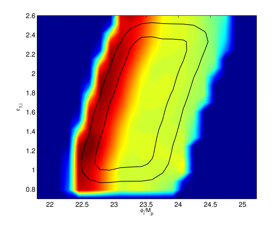
Figure 3: (color online). Degeneracy between $\epsilon_{1,i}$ and $\phi_{i}/M_{p}$ for case 4 in Table LABEL:iep. The contours show the 68$\%$ and 95$\%$ confidence limits of the marginalized posterior distributions. The shading indicates the mean likelihood of samples.

IV.1 Constrained case

From the results for the distributions of cosmological parameters, it is possible to observe that $\epsilon_{1,i}$ and $\phi_{i}$ are degenerate with each other. In order to obtain a better constraints we have varied another instance: keeping $\phi_{i}/M_{P}$ fixed to a certain value and varying $\epsilon_{i,1}$ and $\lambda$, including tensors and lensing and using the TT, TE and EE angular spectra, which is represented by the value of the parameter ($C\ell s=3$). These results were calculated with two chains of 100 000 samples of length each, the best-fit values for this case are shown in Fig. 4 and the results for a $\Lambda$CDM model without tensors and without running is shown in Fig. 5.

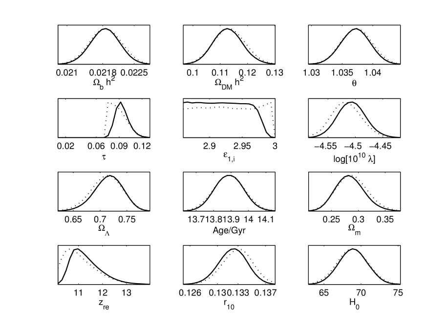
Figure 4: Posterior distributions of cosmological parameters from the prior $\epsilon_{1,i}\in[2.86,2.98]$, $\phi_{i}/M_{p}=25$, $\lambda\in[1.0\times 10^{-12}$,$1.23\times 10^{-12}]$, $C\ell s=3$ with tensors.

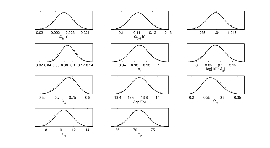
Figure 5: Posterior distributions of cosmological parameters for the ${\rm\Lambda}$CDM model with 6 independent parameters.

The posterior distribution produced a flat distribution of $\epsilon_{1,i}$ and a central value for $\lambda=1.11\times 10^{-12}\pm 0.03$ with a convergence $R-1=0.0008$, an approximate number of 3921 independent samples, and burn in of 40 rows.

We compare our results with a ${\rm\Lambda}$CDM model for 6 parameters: $\Omega_{b}h^{2}$, $\Omega_{DM}h^{2}$, $\theta$, $\tau$, $n_{s}$, $A_{s}$ giving a total of 11 parameters along with $\omega_{\Lambda}$, $\omega_{m}$, $z_{re}$, $H_{0}$ and age of the Universe. That is, we have the same number of primary parameters in the constrained model and one parameter more in the models reported in Table LABEL:iep. Therefore we apply the Akaike information criterion :

$${\rm AIC}=-2\ln{\cal L}_{\rm max}+2N_{\rm par},$$ (11)

in order to compare the goodness of fit of ${\rm\Lambda}$CDM model with the four models reported in Table LABEL:iep. In Eq. 11, ${\cal L}_{\rm max}$ is the maximum likelihood of the model and $N_{\rm par}$ is the number of parameters of that model. This is done in Table 3 .

Table 3: Akaike information criterion applied to results of Table LABEL:iep with respect to a $\Lambda$CDM model of 6 parameters.

Model	$-\ln{\cal L}_{\rm max}$	$N_{\rm par}$	AIC	$\Delta$AIC	$\chi^{2}$
$\Lambda$CDM	3737.2	6	7486.5	0	7474.4
1	3737.4	7	7488.8	2.3	7474.8
2	3737.4	7	7488.8	2.4	7474.8
3	3737.4	7	7488.8	2.3	7474.8

The main difference between the $\Lambda$CDM model and our results comes from the number of parameters ($\Delta N_{\rm par}=1)$. The last column in Table 3, shows the value of a $\chi^{2}$ goodness of fit for these models. Compared to the $\Lambda$CDM model, it differs by $0.4$ which assures that our scenario can fit the data almost as well as $\Lambda$CDM. In terms of the AIC, the $\Lambda$CDM with power-law spectrum without tensors is slightly favored, but not at a significant level.

As observed from Figs. 4, 5, fixing the value of the field has the consequence of changing the shape of the distributions for the reionization redshift $z_{re}$ and the optical depth $\tau$. The initial value of $\epsilon_{1}$ however seems to be allowed to include values lower than 2.9 and we have cut the distribution in accordance to the prior imposed, although the best-fit value is compatible with the argument that a natural $\epsilon_{1,i}$ must be close to 3.

IV.2 Slow-roll predictions

In this section, we apply the results for the initial values of $\epsilon_{1,i}$ and $\phi_{i}/M_{p}$ shown in the last section to calculate the spectra of anisotropies for the CMB and give the values for the inflationary observables calculated at different scales using their slow-roll expressions expanded at first order. We use the following expression to translate the value of the scale $k_{*}$ which represents horizon crossing from GeV to Mpc^-1. This expression was also used in rs for the same purpose and is derived assuming sudden reheating.

$$k_{*}=500\exp^{-\Delta N_{*}}H_{*}\frac{T_{\nu 0}}{T_{reh}}(0.002{\rm Mpc^{-1}}).$$ (12)

The assumption of sudden reheating is implicit in the value of $T_{reh}$ calculated from the temperature at the end of inflation. The predictions for the inflationary observables and the values of the lower multipoles of the CMB for each of the cases presented in Table LABEL:iep are presented in Table LABEL:ri and LABEL:cmb respectively.

Table 4: Values of inflationary observables evaluated at different scales from the result of the Monte Carlo integration. The cases are arranged according to the total amount of inflation produced by each of them.

	Best-fit values: $\epsilon_{1,i}$, $\phi_{i}/M_{p}$, $\lambda$	$N_{T}$		$k_{*}\,(Mpc^{-1})$,   $N_{*}$	$k_{*}\,(Mpc^{-1})$,   $N_{*}$	$k_{*}\,(Mpc^{-1})$,   $N_{*}$
3	2.77,    24.31,    $1.1\times 10^{-12}$	64.31		0.05,    59.4	$1.03\times 10^{-2}$,  61.0	$2.12\times 10^{-3}$,  62.61
			$r$	0.27	0.26	0.28
			$n_{s}$	0.95	0.95	1.26
			$dn_{s}/dlnk$	$-9.0\times 10^{-4}$	$-8.42\times 10^{-3}$	-0.9
4	1.69,    23.43,    $1.1\times 10^{-12}$	64.25		0.055,    59.3	$1.03\times 10^{-2}$,  61.0	$2.15\times 10^{-3}$,  62.6
			$r$	0.27	0.26	0.29
			$n_{s}$	0.95	0.95	1.3
			$dn_{s}/dlnk$	$-9.0\times 10^{-4}$	$-9.77\times 10^{-3}$	-0.97

In Table LABEL:ri $r$, is the tensor to scalar ratio, $n_{s}$ is the spectral index of scalar perturbations and ${\rm d}n_{s}/{\rm d}\ln k$ the running of the spectral index, $N_{T}$ represents the total amount of inflation produced by the model. We present the predictions for the observables on different scales: the first value corresponds to that on which the Monte Carlo integration was done, $0.05$ Mpc^-1. The second to the value that we used in our previous work, $0.01$ Mpc^-1, the third one is that of $0.002$ Mpc^-1, where the analysis of WMAP7 yr is done. $N_{*}$ are different points on the integration trajectories with respect to the number of $e$-foldings where one finds the corresponding value of $k_{*}$ by using Eq. 12. In a previous work rs , we compared the slow-roll trajectories obtained by the WMAP team to those of this scenario in the $n_{s}$-$r$ plane. We showed that the modified initial conditions lead to an increase of the spectral index at the largest scales, in such a way that allows the $\lambda\phi^{4}$ potential to be allowed by current data.

IV.3 CMB Anisotropies

We intend to see whether the suppression of power on large scales on the primordial power spectra produced by this scenario as seen in rs could explain the lack of correlation on large angular scales in the lower multipoles of the CMB, Spergel , Copi , Copi2 . There are other works that explore the effects of different inflationary setups to explain the lack of power at low multipoles of the CMB: using a fitting function and a cut off in a fast-roll era bdvs , a primordial magnetic field bh , anisotropic inflation gcp , using a curvaton model frv and isocurvature perturbations, gh . In our work, we do not fit the primordial power spectra, but allow the numeric solution of the mode and background equations to fully determine its shape. We use the initial conditions for the background dynamics, determined through the Monte Carlo integration, to calculate the value of the pivot scale on which perturbations are evaluated using their slow-roll expressions. The assumption of sudden reheating to obtain the value of the pivot scale in $Mpc^{-1}$ gives an uncertainty on these numbers.

There is an important point to mention before presenting the results of this subsection: We obtained the same values for $C_{TT}$ for all pivot scales $k_{*}$ considered in Table LABEL:ri. This is not the case for the standard power-law parameterization of the primordial spectra. In our case, the initial conditions for the mode integration are not dependent on the value of the pivot scale. We do not use this value because the scenario we are investigating is not in the slow-roll regime at horizon crossing and therefore, setting initial conditions at horizon crossing, even if they violate slow-roll do not assure us that we are going to recover those initial values which characterize this scenario.

The values of the multipole moments $C_{\ell}$ do change slightly for different initial conditions of $\epsilon_{1}$ and $\phi/M_{p}$ in Table LABEL:iep. One can observe however, that those values are not much lower as compared to the standard power-law parameterization and initial inflationary conditions in slow roll. In order to be sure that we were giving the values of the mode integration correctly into the CAMB code, we used the power-law parameterization of the primordial power spectra in our code and the usual slow-roll power-law result of CAMB without any modifications. For the same initial value of the parameters, we checked that the resulting CMB anisotropies for both instances at small scales coincided, as was expected. We had to be careful not to produce a cut-off in the interpolation since it would affect the integration of modes which are deeper subhorizon.

There are some comments to be made in the following about how the choice of initial conditions and the way in which the primordial power spectra are included into the CAMB code.

In order to include the new primordial spectra to calculate the $C_{\ell}$ values, one must interpolate them so that the code can find a wider range of values to the whole range of scales reached by observations. We used the subroutine SPLINT from numerical recipes to interpolate. It turns out that, for some initial conditions in our scenario, this subroutine produces power spectra that are negative. We set this output to 0 as long as this happens. For those initial conditions, one has at large scales that the value of $C_{TT}$ becomes smaller. Then one can either try to fit the quadrupole or octopole separately by trying different initial conditions as the initial $k$ changes, or a bigger value for the first initial $k$. Once this is fixed in the way explained in Sec. II.2, one can choose to use a bigger value for this first scale as it assures that the terms multiplied by $u_{k}$ in Eq. (5) are still positive. We stress that this is not the value for the pivot scale at horizon crossing used for the Monte Carlo integration but the value of the first mode to be integrated at the beginning of inflation.

If one is exploring parameter space for $\epsilon_{1,i}$ and $\phi_{i}/M_{p}$, one has to be careful not to hit regions in which the amount of inflation produced is too small. This can either happen for a fixed $\phi_{i}/M_{p}$ that gives enough inflation for a certain value of $\epsilon_{1,i}$ and as the later goes closer and closer to 3 the amount of total inflation is reduced, or for a fixed $\epsilon_{1,i}$ and a small value of the field. Both situations cause the interpolation to produce again a negative power spectra.

Table 5: Predicted CMB band power $\Delta T_{\ell}=\ell(\ell+1)C_{\ell}/2\pi$ of quadrupole and octopole for all best-fit models shown in Table LABEL:iep2.

	$\Delta T_{2}/\mu$K2	$\Delta T_{3}/\mu$K2
1	1 228	1 139
2	1 234	1 146
3	1 228	1 140
4	1 228	1 140

Having these situations in mind, one can find either initial conditions that fit the value of the quadrupole and the octopole separately, or increase the value of the initial scale to be considered for the mode integration so that the final output gives less power in the lower multipoles, this would be a complementary way to compensate for the situation mentioned at the beginning of this subsection. The value of the pivot scale considered in CAMB does not have any influence in the mode integration, but one can consider varying the value of the first scale to be integrated as long as the equations for the perturbations are well defined. However, we have not explored further this last situation and its consequences for the inflationary observables and the Monte Carlo integration.

If one tries the first method, the result is that the upper multipoles are misplaced, this is different from the result found in ws where they use a $\chi^{2}$ distribution to fit the CMB and different initial values for the scale factor considering a preinflationary radiation dominated epoch. Those initial conditions that enter in the first possibility are listed in Figure 6.

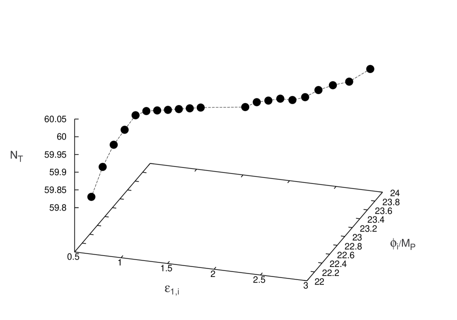
Figure 6: Initial conditions in concordance with the observed CMB quadrupole.

By keeping the value of $\epsilon_{1,i}$ fixed and finding the value of $\phi_{i}/M_{p}$ that gives the desired result for $\ell=2$, we found that as long as $\epsilon_{1,i}>1$, this happened always at a value of $\phi_{i}/M_{p}$ that gave the same amount of total inflation. Once $\epsilon_{1,i}<1$ we did not find the same effect.

By increasing instead the value of the initial scale to be considered for the mode integration by a factor of 60, one can reduce the values of the quadrupole and octopole arriving to values as low as 346.7 for $\ell=2$ and 344.7 for $\ell=3$. The values are the lowest ones obtained even if one uses bigger scales. In some of those cases the interpolation again gives negative values for the output of the primordial power spectra and for other values of $k_{min}$, which could be bigger or smaller, gives a positive output throughout the whole interpolation process. The quadrupole and octopole could no be fit at the same time.

For all the models that fit the quadrupole and octopole by trying different initial conditions, there is a range of $N_{*}$ or equivalently, of pivot scales in which the inflationary observables $r,n_{s},dn_{s}/dlnk$ are inside the $1\sigma,2\sigma,1\sigma$ intervals respectively, for WMAP7 with running and tensors, but not the amplitude of scalar perturbations, which turns out to be very small : $2.11\times 10^{-9}$ in the best of cases, even for those initial conditions with $\epsilon_{1,i}<1$. For the octopole on the contrary, the amplitude is too big : $3.31\times 10^{-9}$.

IV.4 Mode Integration results

Some comments on the results of the mode integration are made in this subsection. We have mentioned before that for a fixed initial value of the field, the bigger $\epsilon_{1,i}$ is or closer to 3, the less amount of total inflation produced by the model there is. If one keeps fixed instead the value of the scalar field, in order to have more inflation produced, the value of $\epsilon_{1,i}$ has to be decreased. That is, $\epsilon_{1,i}$ and $\phi_{i}/M_{p}$ are correlated and the only free parameter is the total amount of inflation produced $N_{T}$. For a fixed amount of total inflation,the bigger $\epsilon_{1,i}$ is, the bigger the initial value of the field must be in order to compensate.

For the mode integration of perturbations, we fixed the initial value of the scale factor to 1 at the beginning of inflation. As in this scenario there is an epoch of noninflationary expansion, we discarded the number of $e$-foldings during that time and reset it to 0 at the beginning of inflation.

In Figs. 7 and 8 we present examples for the primordial scalar and tensor power spectra as obtained from a mode-by-mode integration and compared to the corresponding slow-roll predictions.

Figure 7: Scalar power spectrum for the initial condition $\epsilon_{1,i}=2.93$, $\phi_{i}/M_{p}=24.67$, $\lambda=1\times 10^{-12}$. The main plot shows the scales in the x-axis in GeV, the subplot in Mpc^-1.

Figure 8: Tensor power spectrum for the initial condition $\epsilon_{1,i}=2.93$, $\phi_{i}/M_{p}=24.67$, $\lambda=1\times 10^{-12}$. The main plot shows the scales in the x-axis in GeV, the subplot in Mpc^-1.

We can observe oscillations in the amplitude of the scalar and tensor perturbations. We have seen before that the initial value of the first mode to be integrated is already very close to horizon crossing due to the way it is chosen for this scenario. This means, that we are still able to observe the sub horizon oscillations of the solutions in Eq. (5) before the growing mode dominates. In ws , it is said that those oscillations disappear by considering an initial condition for the scale factor deeper into a previous epoch of radiation domination. We are not considering this situation here. However, we have checked that if one chooses a bigger initial scale to do the mode integration, the cutoff and oscillatory behavior observed before disappear completely and the mode integration and slow-roll spectra are the same for all scales. That is, one obtains pure power-law spectra.

V summary and discussion

The idea of considering a limited amount of inflationary expansion as a modification of the chaotic inflation scenario implies a choice of initial conditions that have observable consequences. In this scenario, the kinetic energy dominates before the onset of inflation and consequently violates the slow-roll conditions at horizon crossing of observable modes before the system joins the inflationary attractor.

The best-fit power spectrum of scalar perturbations shows a sharp cutoff on large scales. This however, does lead to a significant suppression of the angular CMB power at the largest angular scales. The reason is that the cutoff in a $\lambda\phi^{4}$ model with just enough $e$-foldings turns out to be at scales that are too large to account for a lack of power in the CMB at the largest angles. However, one can obtain values very close to those of the reported quadrupole and octopole by considering bigger values of the initial scale to be integrated, and also by tuning the initial conditions to find them separately. This, however, causes higher multipoles to have much higher values than observed. However these results are only applicable for the $\lambda\phi^{4}$ potential.

The results of the mode integration for the tensor modes show that they have less power, as expected, than the scalars and their power spectrum also shows a sharp cutoff at large scales.

An interesting point concerning the initial conditions of the inflaton and $\epsilon_{1}$ is that the Monte Carlo integration gives predictions of best-fit values only for those intervals specified in the priors. It does not give information about the physical significance of the region explored, unless that information is contained in the amount of independent samples given by the simulation for different distributions. We have seen that values $\epsilon_{1,i}\approx 3$ give bigger numbers of independent samples.

The Monte Carlo integration confirms in the sense mentioned above, that a natural initial condition for this scenario corresponds to the first horizon flow function being close to 3. We have already seen that an initial epoch of kinetic energy domination naturally leads to this initial condition.

We have been able to prove with the results obtained by the Monte Carlo integration, that the $\lambda\phi^{4}$ potential is inside current observational constraints for single-field models of inflation.

The implementation of this scenario still lacks the consideration that the initial conditions for the perturbations cannot be in the Bunch–Davies vacuum and that the equations of motion for the background are approximated by a flat homogeneous Universe. Both should be reconsidered in order to have consistency with the fact that there is kinetic energy domination at the beginning of inflation. However, as a first approach, we could obtain enough information of the main behavior for the inflationary observables and the predictions for the CMB anisotropies given by this scenario. One should be able now to apply it to different potentials and explore more general situations and their consequences.

VI acknowledgments

This research was supported by the DFG cluster of excellence ”Origin and Structure of the Universe”. We thank the advice and help with the numerics of Jürgen Engels, Rossella Falcone, Tommaso Giannantonio, Zong-Kuan Guo, Martin Kilbinger, Julien Lesgourgues, Alexey Mints, Aravind Natarajan, David Parkinson, Christophe Ringeval, Jussi Valiviita and Wessel Valkenburg. E. R. acknowledges the use of the Linux Cluster of the Leibniz-Rechenzentrum der Bayerischen Akademie der Wissenschaften and the help of Reinhold Bader and Orlando Rivera. We used the CAMB and COSMOMC packages as well as WMAP 7-yr data from the LAMBDA server.

References

- (1) E. Komatsu et al. (WMAP Collaboration), Astrophys. J. Suppl. 192, 18 (2011).
- (2) A. D. Linde, Phys. Lett. 129B, 177 (1983).
- (3) C. R. Contaldi, M. Peloso, L. Kofman and A. Linde, J. Cosmol. Astropart. Phys. 07 (2003) 002.
- (4) D. Boyanovsky, H. J. de Vega and N. G. Sanchez, Phys. Rev. D 74, 123007 (2006); C. Destri, H. J. de Vega and N. G. Sanchez, Phys. Rev. D 78, 023013 (2008); F. J. Cao, H. J. de Vega and N. G. Sanchez, Phys. Rev. D 78, 083508 (2008); C. Destri, H. J. de Vega and N. G. Sanchez, Phys. Rev. D 81, 063520 (2010).
- (5) I. C. Wang and K. W. Ng, Phys. Rev. D 77, 083501 (2008).
- (6) B. A. Powell and W. H. Kinney, Phys. Rev. D 76, 063512 (2007).
- (7) J. F. Donoghue, K. Dutta and A. Ross, Phys. Rev. D 80, 023526 (2009).
- (8) D. J. Schwarz and E. Ramirez, arXiv:0912.4348.
- (9) E. Ramirez and D. J. Schwarz, Phys. Rev. D 80, 023525 (2009).
- (10) A. Lewis, A. Challinor, and A. Lasenby, Astrophys. J. 538, 473 (2000).
- (11) A. Lewis and S. Bridle, Phys. Rev. D 66, 103511 (2002).
- (12) D. J. Schwarz, C. A. Terrero-Escalante, and A. A. Garcia, Phys. Lett. B 517, 243(2001) .
- (13) W. H. Kinney, Phys. Rev. D 66, 083508 (2002); A. R. Liddle, Phys. Rev. D 68, 103504 (2003); N. Agarwal and R. Bean, Phys. Rev. D 79, 023503 (2009).
- (14) A. D. Linde, Contemp. Concepts Phys. 5, 1 (2005); A. D. Linde, Particle Physics and Inflationary Cosmology, (Harwood Academic Publishers, Chur, Switzerland, 1990), chap. 9.
- (15) V. F. Mukhanov, H. A. Feldman and R. H. Brandenberger, Phys. Rept. 215, 203 (1992).
- (16) S. M. Leach, A. R. Liddle, J. Martin and D. J. Schwarz, Phys. Rev. D 66, 023515 (2002).
- (17) J. Lesgourgues, A. A. Starobinsky and W. Valkenburg, J. Cosmol. Astropart. Phys. 01 (2008) 010.
- (18) A. Gelman, D. B. Rubin, Statist. Sci., 7, 457 (1992).
- (19) G. Hinshaw, A. J. Banday, C. L. Bennett, K. M. Górski, A. Kogut, C. H. Lineweaver, G. .F. Smoot, and E. L. Wright, Astrophys. J. Lett. 464, L25 (1996); D. N. Spergel et al. (WMAP Collaboration), Astrophys. J. Suppl. Ser. 148, 175 (2003).
- (20) C. J. Copi, D. Huterer, D. J. Schwarz and G. D. Starkman, Mon. Not. R. Astron. Soc. 399, 295 (2009).
-
(21)
D. J. Schwarz, G. D. Starkman, D. Huterer
and C. J. Copi, Phys. Rev. Lett. 93, 221301 (2004); C. Copi, D. Huterer, D. Schwarz and G. Starkman, Phys. Rev. D 75, 023507 (2007). -
(22)
D. Boyanovsky, C. Destri, H. J. De Vega and
N. G. Sanchez, Int. J. Mod. Phys. A 24, 3669 (2009). - (23) A. Bernui and W. S. Hipolito-Ricaldi, Mon. Not. R. Astron. Soc. 389, 1453 (2008).
- (24) A. E. Gumrukcuoglu, C. R. Contaldi and M. Peloso, J. Cosmol. Astropart. Phys. 11 (2007) 005, arXiv:astro-ph/0707.4179; A. E. Gumrukcuoglu, C. R. Contaldi and M. Peloso, astro-ph/0608405.
- (25) F. Ferrer, S. Rasanen and J. Valiviita, J. Cosmol. Astropart. Phys. 10 (2004) 010.
- (26) C. Gordon and W. Hu, Phys. Rev. D 70, 083003 (2004).