Quantum astrometric observables I: time delay in classical and quantum gravity

Abstract

A class of diffeomorphism invariant, physical observables, so-called astrometric observables, is introduced. A particularly simple example, the time delay, which expresses the difference between two initially synchronized proper time clocks in relative inertial motion, is analyzed in detail. It is found to satisfy some interesting inequalities related to the causal structure of classical Lorentzian spacetimes. Thus it can serve as a probe of causal structure and, in particular, of violations of causality. A quantum model of this observable as well as the calculation of its variance due to vacuum fluctuations in quantum linearized gravity are sketched. The question of whether the causal inequalities are still satisfied by quantized gravity, which is pertinent to the nature of causality in quantum gravity, is raised, but it is shown that perturbative calculations cannot provide a definite answer. Some potential applications of astrometric observables in quantum gravity are discussed.

I Introduction

The issue of physical observables in both classical and quantum theories of gravity has been a topic of long standing interest both practically and theoretically. Practically, precise models for tracking the positions of objects on scales from Solar System to cosmological require input from general relativity. Such models go under the generic name of relativistic astrometry Soffel (1989). Also, models of the very early Universe rely on incorporating quantum gravitational effects in order to predict potentially observable signatures in current cosmological observations (Sec. 5.7 of Woodard (2009)). Theoretically, the algebra of physical observables, with each observable a mathematical model of an experimental outcome, is an integral part of a complete classical or quantum theory of gravity Bergmann (1961); Rovelli (1991); Lusanna and Pauri (2006); Dittrich (2006); Dittrich and Tambornino (2007); Pons et al. (2010). In each of these cases, one has to confront the problem that, while physical observables are expected to be invariant under spacetime diffeomorphisms, in the usual formulation of general relativity everything is described in terms of tensor fields, which are covariant but not invariant under spacetime diffeomorphisms.

A resolution of the problem of physical observables would then involve two parts. First, one has to explicitly describe a sufficiently large class of spacetime diffeomorphism-invariant (or diff-invariant) quantities expressed in terms of tensor fields. Second, one has to identify elements of this class that correspond to outcomes of some experiments of interest. The literature on this subject is extensive Bergmann (1961); Rovelli (1991); Lusanna and Pauri (2006); Dittrich (2006); Dittrich and Tambornino (2007); Giddings et al. (2006); Pons et al. (2010) (see also references therein), but no solution has been entirely successful. To illustrate the difficulties, consider the following two examples. A simple-to-describe class of diff-invariant quantities consists of the spacetime integrals of the form

$$\int_{M}f(g,\phi)\,v_{g},$$ (1)

where $M$ is the entire spacetime, $f$ is some smooth spacetime scalar defined only in terms of the metric $g$ and other dynamical fields $\phi$, and $v_{g}$ is the metric volume form. Unfortunately, even ignoring the issue of convergence of such integrals, this class of diff-invariant quantities is not rich enough to describe the outcomes of any experiments that we are likely to perform (since such experiments would necessarily be localized in a finite region of spacetime). The other example is more abstract. Consider (formally) the physical phase space of general relativity defined as the quotient by spacetime diffeomorphisms of the space of solutions of Einstein’s equations. Ostensibly, any function on this space is a diff-invariant quantity, and hence a physical observable. Moreover, all physical observables are so captured. However, due to the abstract nature of this construction, it is not possible to assign a clear physical meaning to any element of this class. There is, a priori, no effective way to specify an individual element of this class or to carry out practical calculations with it.

The aim of this work is to take a pragmatic approach to the explicit construction of physical observables and apply it to more theoretical problems like studying the causal structure of quantum gravity. From a theoretical point of view, the abstract notion of a physical observable, sketched in the previous paragraph, as a function on the physical phase space is quite satisfactory. The main problem remaining is to identify observables of interest and given them a physical interpretation in terms of a modeled experimental outcome. A natural way of addressing this difficulty, inspired by the methods used in practical problems like relativistic astrometry, is to start with a potential experiment in mind and construct a sufficiently detailed mathematical model of it. Such a model should include sufficiently many dynamical variables representing parts of the experimental apparatus such that the desired measurement outcome can be modeled using the relative configurations of these variables. The result is a mathematical model of a measurement outcome, in other words a physical observable. This observable, by virtue of its operational definition, should then be a diff-invariant quantity and thus an element of the algebra of functions on the physical phase space of the theory. Now though, fortunately, since we started out by modeling an experiment, its physical interpretation is clear.

A mathematical model of an experiment interacting with dynamical gravity is likely to make reference to solutions of geodesic or wave equations on unspecified (indeed dynamical) metric backgrounds. Coupled with the large variety of experiments that could be imagined and modeled, a remaining practical difficulty is that the resulting physical observable is still specified only implicitly and may not be immediately amenable to practical calculations. It appears that this problem can only be overcome on a case by case basis. For the particular observable considered in this work, the time delay, this difficulty is overcome by appealing to perturbation theory and providing explicit formulas, based on an exact implicit definition, in terms of one-dimensional integrals over linear metric perturbations about Minkowski space.

The idea of using operationally or “relationally” defined observables in gravitational theories is not entirely novel. It has been previously considered in Rovelli (2002, 2004); Dittrich (2006). Unfortunately, that work has remained at a rather abstract level and did not make use of sufficiently realistic experimental models, thus keeping the physical interpretation of the constructed observables somewhat moot. The previous works that used ideas most similar to ours are Ford (1995), Ohlmeyer (1997), and . Unfortunately, the original work of Ford (1995) and its follow-ups Yu and Ford (1999); Borgman and Ford (2004); Thompson and Ford (2006), while exhibiting a clear physical interpretation, left many mathematical loose ends. In particular, the issues of diff-invariance (or gauge invariance) and regularization were not treated entirely satisfactorily, both of which are explicitly addressed in this work, see Secs. V.2.3 and VI.3.2. Another work in a similar spirit is Tsamis and Woodard (1992), especially at the technical level, though with a different physical motivation. On the other hand, the original work Woodard (1984) gives several different motivations for the technical calculations, including an approach very similar to that of this paper in terms of the construction of diff-invariant, physically meaningful gravitational observables. At the technical level, the main departure of this work from that of Woodard (1984); Tsamis and Woodard (1992) is in the use of smeared observables to regularize divergences appearing due to the use of geodesics of idealized, point-like particles, see Sec. VII.3.

In Sec. II, we operationally define the time delay physical observable (or rather a family of related observables). Section III gives an exact, though implicit, mathematical model for this physical observable in a theory of gravity coupled to a minimal amount of matter modeling the experimental apparatus. Section IV contains an analysis of why the time delay is an observable interesting for studying the causal structure of gravity. In particular, two important inequalities are derived directly from the Lorentzian character of the metric field. Section V, using technical results on the perturbative solution of the geodesic and parallel transport equations presented in the Appendix, gives an explicit formula for the time delay in linearized gravity. Sections VI and VII sketch how the time delay should be defined as a quantum observable and how explicit calculations in linearized quantum gravity can capture some aspects of causal structure of quantum gravity. Due to the added complexity of quantum mechanics, these two sections are naturally less detailed than the preceding ones. The issues discussed in these sections will be addressed in more detail elsewhere. Section VIII concludes with a discussion of the results and an outlook to future work.

II Operational description and gauge invariance

The time delay observable is defined by the following experimental protocol, Fig. 1 (which is of course only an idealization of a real experiment). Consider a laboratory in inertial motion (free fall). The laboratory carries a clock that measures the proper time along its trajectory. The laboratory also carries an orthogonal frame, which is parallel-transported along the lab’s worldline. (The frame could be Fermi-Walker-transported if the motion were not inertial.) At a moment of the experimenter’s choosing, the lab ejects a probe in a predetermined direction, fixed with respect to the lab’s orthogonal frame and with a predetermined relative velocity. The probe then continues to move inertially and carries its own proper time clock. The two clocks are synchronized to $0$ at the ejection event $O$. After ejection, the probe continuously broadcasts its own proper time (time stamped signals), in all directions using an electromagnetic signal (which hence travels at the speed of light). At a predetermined proper time interval $s$ after ejection, event $Q$, the lab records the probe signal and its emission time stamp $\tau(s)$, sent from event $P$. Call $s$ the reception time, $\tau(s)$ the emission time and the difference

$$\delta\tau(s)=s-\tau(s)$$ (2)

the time delay.

Figure 1: Geometry of the experimental protocol defining the reception time $s$, emission time $\tau(s)$, and the time delay $\delta\tau(s)=s-\tau(s)$. The synchronization/ejection point is $O$. The signal emission point is $P$ and the signal reception point is $Q$.

The time delay $\delta\tau(s)$ as well as the emission and reception time are presumed to have been measured with negligible inaccuracy. Of course, that is a severe idealization. For it to be reasonable, the magnitude of $\delta\tau(s)$ must exceed the noise from the intrinsic inaccuracies in the probe and lab instruments (clocks, gyroscopes, ejection mechanism, transmission and recording uncertainties, etc.). Given the smallness of both the classical and quantum contributions to $\delta\tau(s)$ (which are suppressed by all of the following: magnitude of light speed, smallness of spacetime curvature, and smallness of $\hbar$), is unlikely to be reasonable in our own Universe, at least for naïve ways to realize this experimental setup.

However, there is no a priori reason for not being able to perform such measurements successfully with (significantly) more clever or improved experimental techniques, or in a universe with different values of some of the fundamental constants. A successful theory of quantum gravity should be able to yield quantitative predictions (for any universe) for this and related observables. Some set of these observables may actually be practically measurable in our own Universe. As such, the time delay, by virtue of its simplicity and ease of physical interpretation, serves as a useful benchmark for dealing with whatever practical difficulties are likely come up in calculations involving similar, but perhaps more realistic, observables.

III Classical mathematical model

A significantly idealized mathematical model of the experiment described in the preceding section, in the classical theory, consists of the geometrical objects collected in the following definition.

Definition 1.

A lab-equipped spacetime $(M,g,O,e^{a}_{i})$ consists of an oriented, Lorentzian, time-oriented, globally hyperbolic, $n$-dimensional spacetime $(M,g)$, a point $O\in M$ and an oriented orthonormal frame $e^{a}_{i}\in T_{O}M$, with $a$ an abstract tensor index and $i=0,1,\ldots,n$, where $e^{a}_{0}$ is timelike and future-directed.

See Sec. 2.4 of Wald (1984) for the distinction between abstract and coordinate tensor indices. Physically, the point $O$ represents the spacetime event when the probe is ejected from the lab. The vector $e^{a}_{0}$ is tangent to the lab’s worldline and $e^{a}_{i}$, $i=1,2,\ldots,n$ is the oriented spatial frame carried by the lab. Note that the restrictions on the Lorentzian geometry of $(M,g)$ may not all be necessary. Also, in this work we only consider the case $n=4$.

Of course, due to the background independence of gravitational physics, the measurements carried out in spacetimes related by diffeomorphisms (i.e., gauge transformations) must be identical. It is thus useful to introduce the following notion of equivalence.

Definition 2.

Two lab-equipped spacetimes $(M,g,O,e^{a}_{i})$ and $(M^{\prime},g^{\prime},O^{\prime},e^{\prime a}_{i})$ are gauge equivalent if there exists a diffeomorphism $\chi\colon M\to M^{\prime}$ such that $\chi_{*}g=g^{\prime}$, $\chi(O)=O^{\prime}$ and $\chi_{*}e^{a}_{i}=e^{\prime a}_{i}$, where $\chi_{*}$ denotes the differential push-forward.

An observable is modeled mathematically by a function on the space of lab-equipped spacetimes. The time delay observable is defined by implementing the protocol outlined in the preceding section. First, we need the following further definitions.

Definition 3.

The lab worldline, $Q(s)=\exp_{O}(su)$, is the geodesic passing through $O$ with tangent vector $u^{a}=e^{a}_{0}$. Here $\exp_{O}\colon T_{O}M\to M$ is the usual geodesic exponential map.

The probe worldline, $P(t)=\exp_{O}(tv)$, is the geodesic passing through $O$ with tangent vector $v^{a}=v^{i}e^{a}_{i}$, with $v^{i}\in\mathbb{R}^{1,3}$ a timelike, future-directed, unit vector, chosen independent of the spacetime geometry.

The signal worldline, $Z(t,\lambda)$, is the null geodesic emanating from a point on the probe worldline, $Z(t,1)=P(t)$, and intersecting the lab worldline, $Z(t,0)=Q(s)$, with the earliest possible $s$ (alternatively, if $s$ is fixed, then $t$ is chosen to be the latest possible).

The values of $t$ and $s$ connected by $Z$ are functionally related. This relationship defines the time delay observable.

Definition 4.

If $t$ and $s$ are such that $P(t)$ and $Q(s)$ are connected by $Z(t,\lambda)$, they are referred to as a pair of emission and reception times. The functional relationship between them is denoted

$$t=\tau_{v}(s),$$ (3)

where $\tau_{v}(s)$ is called the recorded emission time and the difference

$$\delta\tau_{v}(s)=s-\tau_{v}(s),$$ (4)

is called the time delay.

By construction, the following theorem holds.

Theorem 1.

Given two gauge-equivalent lab-equipped spacetimes $(M,g,O,e^{a}_{i})$ and $(M^{\prime},g^{\prime},O^{\prime},e^{\prime a}_{i})$, the corresponding time delays (keeping $s$ and $v^{i}$ fixed) are equal:

$$\delta\tau_{v}(s)=\delta\tau^{\prime}_{v}(s).$$ (5)

In other words, the time delay (as well as as any function thereof, such as the recorded emission time) constitutes a genuine (diffeomorphism-invariant) physical observable on lab-equipped spacetimes. When the context is clear, we will omit the explicit dependence of $\delta\tau_{v}(s)$ on $v$ or $s$.

IV Causal inequalities

The time delay is interesting in more ways than just being an explicit example of a physical observable sensitive to the ambient gravitational field. The experimental protocol defining it can be thought of as designed to test the impossibility of superluminal signal propagation and the geodesic character of the lab worldline. In particular, under quite generic assumptions related to the Lorentzian character of spacetime geometry, the time delay satisfies inequalities that would be violated if the above-mentioned tests were to fail. A careful examination of a mathematical model of such tests for classical spacetimes can serve as a benchmark to understand possible outcomes of such tests in any proposed theory of quantum spacetime.

IV.1 Maximality of light speed

In curved spacetimes, it is impossible to objectively compare the speed of light at different spacetime events. Due to general covariance, any experiment to measure the local speed of light, calibrated at spacetime event $x$ to return the value $1$, will return the same value $1$ at any other spacetime event $y$, provided it was parallel-transported there. Therefore any such experiment must perform measurements in finite regions of spacetime.

In the case of the time delay experiment, since light is used to send the signals, the local speed of signal propagation cannot by definition exceed that of light. However, to take into account possible nontrivial global geometry, we adopt the following definition of (apparent) superluminal signal propagation. Consider a pair of emission-reception times $(\tau,s)$. If there exists another pair $(\tau^{\prime},s^{\prime})$ such that $\tau^{\prime}<\tau$ (signal emitted later than $t^{\prime}$) and $s^{\prime}>s$ (signal arrived earlier than $s^{\prime}$), then the later signal must have travelled superluminally, cf. Fig. 2. In classical Lorentzian geometries without closed causal curves we can prove that this never happens.

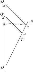
Figure 2: Illustration of the conclusion of Theorem 2. Successive emission times $\tau<\tau$ imply successive reception times $s<s^{\prime}$. The dashed line represents a case, ruled out by the theorem, where the signal might appear superluminal.

Theorem 2.

In a lab-equipped spacetime $(M,g,O,e^{a}_{i})$ we have the following implication between inequalities satisfied by pairs $(\tau(s),s)$ and $(\tau(s^{\prime}),s^{\prime})$ of emission-reception times:

$$\tau(s^{\prime})<\tau(s)~{}\implies~{}s^{\prime}<s.$$ (6)

In particular, when $\tau(s)$ is smooth, we have $\frac{\mathrm{d}}{\mathrm{d}s}\tau(s)>0$.

Essentially, this theorem says that a signal that is emitted later, with respect to the probe, also arrives later, with respect to the lab.

Proof.

Let the two signals be emitted from chronologically successive points $P^{\prime}$ and $P$, and received at points $Q^{\prime}$ and $Q$, respectively. Since $P^{\prime}$ and $P$ are part of the same worldline, $P$ clearly belongs to the set of all points that can be reached from $P^{\prime}$ by future-directed timelike curves, $P\in I^{+}(P^{\prime})$. The points $Q$ and $Q^{\prime}$ are also connected by a timelike curve, though we do not assume in which precedence order, therefore $Q$ must belong to either $I^{+}(Q^{\prime})$ or $I^{-}(Q^{\prime})$. At the same time, by the definition of $Q$, it can be reached by a piecewise smooth, non-spacelike, future-directed curve $P^{\prime}PQ$. Since $P^{\prime}PQ$ is obviously not a null geodesic, Prop. 4.5.10 of Hawking and Ellis (1973) implies that $Q$ and $P^{\prime}$ can be joined by a (future-directed) timelike curve, $Q\in I^{+}(P^{\prime})\subset\operatorname{int}J^{+}(P^{\prime})$. By definition, $Q^{\prime}$ is reached from $P^{\prime}$ by a future-directed null geodesic, such that there is no later point $P^{\prime\prime}$ on the probe worldline with the same property. This implies that $Q^{\prime}\in\partial J^{+}(P^{\prime})$. Otherwise, $Q^{\prime}\in I^{+}(P^{\prime})$, hence $P^{\prime}\in I^{-}(Q^{\prime})$, hence any point $P^{\prime\prime}\in\partial J^{-}(Q^{\prime})$ that is also on the probe worldline violates the preceding hypothesis. But all the timelike curves from $\partial J^{+}(P^{\prime})$ to $\operatorname{int}J^{+}(P^{\prime})\ni Q$ can only be future directed, of which the one reaching $Q$ from $Q^{\prime}$ is a special case, hence $Q\in I^{+}(Q^{\prime})$. This shows that $Q^{\prime}$ chronologically precedes $Q$ or $s^{\prime}<s$. ∎

IV.2 Geodesic extremality

The twin “paradox” is a well-known phenomenon in special relativity: the proper time between two timelike separated events is maximized by a straight line (inertial motion). Its generalization to curved spacetime is generally true only locally: a timelike geodesic maximizes proper time among causal curves close to it (provided it has no conjugate points). Under some conditions on the spacetime or under some extra restrictions on the class of allowed causal curves, geodesic extremality can also hold globally. This includes the special geometry of the time delay experiment. As we shall see below, the time delay observable is also sensitive to some violations of the geodesic extremality. Such violations mimic a breakdown of the equivalence principle (objects no longer fall on geodesics in the absence of external forces).

Figure 3: Illustration of the proof of Theorem 3. The auxiliary dashed curve interpolates between $OQ$ and $OP$, as $\lambda$ varies from $0$ to $1$. As it does so, its proper time length $T(\lambda)$ is shown to decrease monotonically, thus implying $\tau(s)<s$.

Theorem 3.

In a lab-equipped spacetime $(M,g,O,e^{a}_{i})$ (where the lab and probe worldlines are smoothly deformable into each other in a sense to be precised in the proof) a pair $(\tau(s),s)$ of emission-reception times satisfies the inequality

$$\tau(s)<s\quad\text{or equivalently}\quad\delta\tau(s)<0.$$ (7)

Proof.

The basic strategy of the proof is to construct a one-parameter family of piecewise geodesic curves that interpolate between the lab worldline $OQ$ and the probe-signal worldline $OPQ$, while their proper time lengths decrease monotonically, cf. Fig. 3. The existence of the specific interpolation constructed below is the extra technical hypothesis alluded to in the statement of the theorem.

Suppose that the $PQ$ geodesic is affinely parametrized as $Z(\lambda)$, where $Z(0)=Q$ and $Z(1)=P$. Denote also $P_{\lambda}=Z(\lambda)$. Then the family $OP_{\lambda}Q$ clearly interpolates between $OQ$ and $OPQ$, where $OP_{\lambda}$ is a timelike geodesic connecting these points and $P_{\lambda}Q$ is the segment $Z([0,\lambda])$. Since the $P_{\lambda}Q$ segment is null, only the $OP_{\lambda}$ segment contributes to the proper time $T(\lambda)$ along $OP_{\lambda}Q$. Since $T(0)=s$ and $T(1)=\tau(s)$, the proof is concluded as soon as we show that $\frac{\mathrm{d}}{\mathrm{d}\lambda}T(\lambda)<0$, which we do below.

We adapt the calculation of the first variation of the proper time length of a piecewise geodesic curve from Prop. 4.5.4 of Hawking and Ellis (1973). Let $Y(t,\lambda)$ denote the geodesic family $OP_{\lambda}$, parametrized such that $Y(0,\lambda)=O$ and $Y(1,\lambda)=Z(\lambda)$. $Y(t,\lambda)$ is assumed to be smooth in both arguments by the smooth deformability hypothesis of the theorem. Denote $\dot{Y}^{a}=\frac{\partial}{\partial t}Y(t,\lambda)$, $Y^{\prime a}=\frac{\partial}{\partial\lambda}Y(t,\lambda)$ and $f=[-g_{ab}(Y(t,\lambda))\dot{Y}^{a}\dot{Y}^{b}]^{1/2}$. Also, for the purposes of the calculation below, pick a coordinate chart $x^{\alpha}$ and replace the Latin abstract tensor indices by Greek coordinate indices.

$$f^{\prime} =-f^{-1}\left[g_{\alpha\beta}\dot{Y}^{\prime\alpha}\dot{Y}^{\beta}+\frac{1}{2}g_{\alpha\beta,\gamma}Y^{\prime\gamma}\dot{Y}^{\alpha}\dot{Y}^{\beta}\right]$$ (8)

$$=-\dot{Y}^{\prime\gamma}g_{\gamma\beta}\frac{\dot{Y}^{\beta}}{f}-Y^{\prime\gamma}\frac{1}{2}g_{\alpha\beta,\gamma}\frac{\dot{Y}^{\alpha}\dot{Y}^{\beta}}{f}$$ (9)

$$=-\frac{\partial}{\partial t}\left(g_{\alpha\beta}Y^{\prime\alpha}\frac{\dot{Y}^{\beta}}{f}\right)$$ (10)

$$\quad{}+fY^{\prime\gamma}\left[\frac{1}{f}\frac{\partial}{\partial t}\left(g_{\gamma\beta}\frac{\dot{Y}^{\beta}}{f}\right)-\frac{1}{2}g_{\alpha\beta,\gamma}\frac{\dot{Y}^{\alpha}\dot{Y}^{\beta}}{f^{2}}\right]$$

$$=-\frac{\partial}{\partial t}\left(g_{ab}Y^{\prime a}\frac{\dot{Y}^{b}}{f}\right).$$ (11)

Note that the bracketed term vanished because it is precisely the geodesic condition (Eq. 87.3a of Landau and Lifshitz (1980)) and $Y(t,\lambda)$ is a geodesic for fixed $\lambda$. At $t=0$, we have $Y^{\prime a}=0$, while at $t=1$, we have $Y^{\prime a}=Z^{\prime a}$, which is a past-directed null vector.

$$T^{\prime}(\lambda) =\frac{\partial}{\partial\lambda}\int_{0}^{1}\mathrm{d}{t}\,[-g_{ab}\dot{Y}^{a}\dot{Y}^{b}]^{1/2}=\int_{0}^{1}\mathrm{d}{t}\,f^{\prime}$$ (12)

$$=-\int_{0}^{1}\mathrm{d}{t}\,\frac{\partial}{\partial t}\left(g_{ab}Y^{\prime a}\frac{\dot{Y}^{b}}{f}\right)$$ (13)

$$=-g_{ab}Z^{\prime a}\frac{\dot{Y}^{b}}{f}<0.$$ (14)

The latter inequality follows because $\dot{Y}^{a}/f$ is a future-directed timelike unit vector and $Z^{\prime a}$ is a past-directed null vector, hence their inner product is positive. Armed with this inequality, it immediately follows that

$$s-\tau(s)=T(0)-T(1)=-\int_{0}^{1}\mathrm{d}\lambda\,T^{\prime}(\lambda)>0,$$ (15)

which completes the proof. ∎

V Explicit calculation in classical linearized gravity

The time delay observable, while well-defined from its description in the preceding sections, has so far been defined only implicitly. Unfortunately, it would be very difficult to obtain an explicit expression for it, except in highly symmetric spacetimes, where the required geodesics can be computed explicitly. In particular, in Minkowski space, as is done below, it can be computed by elementary means. Fortunately, for small perturbations of Minkowski space, an explicit expression for the time delay can be found at linear order. Such an expression would be especially needed for the calculation of quantum averages and fluctuations, as sketched in Sec. VII.

The calculations are carried out in the tetrad formalism. While linearized gravity calculations are usually carried out in the more familiar metric variables, there are a few reasons to consider tetrads. Using tetrads opens the door to a kind of improved perturbation theory, where the metric keeps its Lorentzian signature at every step of the approximation. This line of investigation, as briefly brought up in Sec. VIII, will be pursued elsewhere. Another advantage of tetrads is that they are needed in the standard way of formulating fermions on curved spacetime.

First, we explicitly compute the time delay in Minkowski space and check the causal inequalities. Then, using the results of the perturbative solution of the geodesic and parallel transport equations of the Appendix, we compute the explicit expression for the time delay at linear order in the deviation from Minkowski space.

V.1 Minkowski space

Consider Minkowski space $(M=\mathbb{R}^{4},\eta,0,\hat{x}^{a}_{i})$, with $\eta=\mathrm{diag}(-1,1,1,1)$, as a lab-equipped spacetime. Without loss of generality, we can take an arbitrary inertial coordinates $x^{i}$ on $(M,\eta)$ and use their origin $0$ as the synchronization point and the vectors $\hat{x}^{a}_{i}=(\partial/\partial x^{i})^{a}$ as the reference tetrad. The dual tetrad is $\hat{x}^{i}_{a}=(\mathrm{d}x^{i})_{a}$ and satisfies the identities $\hat{x}^{a}_{i}\hat{x}_{a}^{j}=\delta_{i}^{j}$ and $\hat{x}^{a}_{i}\hat{x}_{b}^{i}=\delta^{b}_{a}$. The Minkowski metric is $\eta_{ab}=\eta_{ij}\hat{x}^{i}_{a}\hat{x}^{j}_{b}$.

The lab and probe worldlines are parametrized, respectively, as $x^{i}(s)=su^{i}$ and $x^{i}(t)=tv^{i}$, $i=0,1,2,3$, where $u^{i}=(1,0,0,0)$. Suppose that the relative speed of the two timelike vectors $u^{a}=u^{i}\hat{x}^{a}_{i}$ and $v^{a}=v^{i}\hat{x}^{a}_{i}$ is given by the positive hyperbolic rapidity $\theta$, $v_{\mathrm{rel}}=\tanh\theta$, then we have $u\cdot v=\eta_{ab}u^{a}v^{b}=\eta_{ij}u^{i}v^{j}=-\cosh\theta$. The values of $s$ and $t$ which may be connected by light signals are constrained by

$$\eta_{ij}(su^{i}-tv^{i})(su^{j}-tv^{j}) =0$$ (16)

$$-s^{2}-2st(u\cdot v)-t^{2} =0$$ (17)

$$s^{2}-2st\cosh\theta+t^{2} =0$$ (18)

$$(se^{\theta}-t)(se^{-\theta}-t) =0.$$ (19)

The retarded solution is then

$$\tau_{\mathrm{cl}}(s)=t=se^{-\theta}.$$ (20)

The subscript stands for “classical,” as it will serve in Sec. VII as the classical background expectation for quantum fluctuations. This expression clearly satisfies the causal inequalities obtained in the previous section:

$$\tau_{\mathrm{cl}}(s) =se^{-\theta}<s,$$ (21)

$$\frac{\mathrm{d}}{\mathrm{d}s}\tau_{\mathrm{cl}}(s) =e^{-\theta}>0.$$ (22)

Note that $\theta>0$ since the probe is moving away from the lab. The null vector connecting the emission and absorption points is

$$w^{i}=su^{i}-tv^{i}=s(u^{i}-e^{-\theta}v^{i}).$$ (23)

Another useful identity is

$$v^{i}=e^{\theta}(u^{i}-w^{i}/s).$$ (24)

V.2 Approximately Minkowski space

V.2.1 Tetrad formalism

Consider another lab-equipped spacetime $(M,g,0,\hat{e}^{a}_{i})$, where we have kept the same underlying manifold $M$ and synchronization point $O=0$ as in Minkowski space. On the other hand, we express the new metric as $g_{ab}=\eta_{ij}e^{i}_{a}e^{j}_{b}$, where $e^{i}_{a}$ and $e^{a}_{i}$ is a new dual pair of orthonormal tetrads,

$$e^{a}_{i}e^{b}_{j}g_{ab}=\eta_{ij},~{}e^{a}_{i}e_{a}^{j}=\delta_{i}^{j},~{}e^{a}_{i}e_{b}^{i}=\delta_{a}^{b}.$$ (25)

Using the Minkowski tetrad $\hat{x}^{a}_{i}$ on $M$ as a reference, any other one can be obtained by a local general linear transformation

$$e^{a}_{i}=\bar{T}^{i^{\prime}}_{i}\hat{x}^{a}_{i^{\prime}},~{}e^{i}_{a}=T^{i}_{i^{\prime}}\hat{x}^{i^{\prime}}_{a},$$ (26)

where $T$ and $\bar{T}$ are spacetime-dependent invertible matrices, such that $\bar{T}=T^{-1}$. Similarly, any lab frame $\hat{e}^{a}_{i}$ can be obtained by another general linear transformation at $O$,

$$\hat{e}^{a}_{i}=(T_{O})^{i^{\prime}}_{i}\hat{x}^{a}_{i^{\prime}}.$$ (27)

The possible discrepancy between the lab frame and the spacetime tetrad at $O$ is

$$\hat{e}^{a}_{i}=L^{i^{\prime}}_{i}e^{a}_{i^{\prime}},\quad L^{i^{\prime}}_{i}=(T_{O})^{i^{\prime}}_{j}T^{j}_{i},$$ (28)

where $L$ is clearly a Lorentz transformation, $L^{i^{\prime}}_{i}L^{j^{\prime}}_{j}\eta_{i^{\prime}j^{\prime}}=\eta_{ij}$.

If this new lab-equipped spacetime is approximately Minkowski, then both $T^{i}_{i^{\prime}}$ and $L^{i^{\prime}}_{i}$ must be close to the identity matrix. This is conveniently expressed by first parametrizing them as $T=\exp(h)$ and $L=\exp(h_{O})$, and then requiring that $h$ and $h_{O}$ are close to $0$. The smallness requirement aside, $h$ and $h_{O}$ could be, respectively, an arbitrary matrix and an arbitrary skew-adjoint matrix, $\eta_{ik}(h_{O})^{k}_{j}=-\eta_{kj}(h_{O})^{k}_{i}$. Then the metric is

$$g_{ab} =\eta_{ij}e^{a}_{i}e^{b}_{j}=\eta_{ij}T^{i}_{i^{\prime}}T^{j}_{j^{\prime}}\hat{x}_{a}^{i^{\prime}}\hat{x}_{b}^{j^{\prime}}$$ (29)

$$=\eta_{ab}+(\eta_{i^{\prime}j}h^{i}_{i^{\prime}}+\eta_{ij^{\prime}}h^{j}_{j^{\prime}})\hat{x}_{a}^{i^{\prime}}\hat{x}_{b}^{j^{\prime}}+\mathcal{O}(h^{2})$$ (30)

$$=\eta_{ab}+\tilde{h}_{ab}.$$ (31)

The last two equations describe the relationship between the deviations $h^{i}_{j}$ and $\tilde{h}_{ab}$ from Minkowski space, in the tetrad and metric formalisms respectively,

$$\tilde{h}_{ab}=2h_{(ij)}\hat{x}^{i}_{a}\hat{x}^{j}_{b}+\mathcal{O}(h^{2}),\quad\text{where}\quad h_{ij}=\eta_{ij^{\prime}}h^{j^{\prime}}_{j}.$$ (32)

A worldline $\gamma(t)$ is described by its coordinates $\gamma^{i}(t)=x^{i}(\gamma(t))$. Its tangent vector is denoted $\dot{\gamma}(t)^{a}$. Knowledge of the tangent vector allows one to recover the curve as follows

$$\int_{t_{1}}^{t_{2}}\mathrm{d}{t}\,\dot{\gamma}^{a}(t)(\mathrm{d}{x}^{i})_{a}=\int_{\gamma(t_{1})}^{\gamma(t_{2})}\mathrm{d}{x}^{i}=\gamma^{i}(t_{2})-\gamma^{i}(t_{1}).$$ (33)

For convenience, all curves are affinely parametrized from $0$ to $1$. Thus, the length of a timelike geodesic is equal to the length of its initial tangent vector.

A geodesic $\gamma(t)$ is completely specified by its point of origin $\gamma(0)$ and its initial tangent vector $\dot{\gamma}^{a}(0)$, while a $\gamma$-parallel-transported vector $v^{a}(t)$ is specified by its initial value $v^{a}(0)$ at $\gamma(0)$. Again, for convenience in further calculations, all such initial data are specified with reference to some given curve $\beta$, with $\beta(0)=O$. Namely, the point of origin is $\gamma(0)=\beta(1)$, the initial tangent vector $\dot{\gamma}^{a}(0)$ is the $\beta$-parallel-transported image of a vector $\dot{\gamma}^{a}_{O}=\dot{\gamma}^{i}_{O}\hat{e}^{a}_{i}$, and the initial value $v^{a}(0)$ is the $\beta$-parallel-transported image of a vector $v^{a}_{O}=v^{i}_{O}\hat{e}^{a}_{i}$ (cf. Fig. 7). The geodesic and parallel transport equations are written down and solved to order $\mathcal{O}(h)$ in the Appendix.

V.2.2 Geodesic triangle construction

All curves considered in this section are perturbations of piecewise linear paths, which are piecewise geodesic in Minkowski space. In particular, at zeroth order in $h$, the sides of the geodesic triangle formed by the worldlines of the lab, the probe, and the signal form an ordered sequence of spacetime segments $(V,W,U)$, as illustrated in Fig. 4. Namely, $V$ stretches from $O$ to $P$, $W$ stretches from $P$ to $Q$, and $U$ stretches from $Q$ back to $O$. Using the convention of the last paragraph of the preceding section, each of the $(V,W,U)$ segments can be specified as starting from the end point of the preceding one (note that the order corresponds to counterclockwise starting from $O$ in Fig. 4) with the respective tangent vectors $(tv^{a},w^{a},-su^{a})$. Because Minkowski space is flat, it is clear that the segments $VWU$ form a closed triangle by virtue of their tangent vectors adding up to zero.

In approximately Minkowski space, we wish to describe a perturbed version of the above construction. Namely, a sequence of geodesic segments $(\tilde{V},\tilde{W},\tilde{U})$, connected from end to end, with the respective images $(\tilde{t}\tilde{v}^{a},\tilde{w}^{a},-\tilde{s}\tilde{u}^{a})$ of their initial tangent vectors parallel-transported to $O$. We take $\tilde{u}^{a}$ and $\tilde{v}^{a}$ to be unit vectors, hence $\tilde{s}$ and $\tilde{t}$ are the proper time lengths of the corresponding segments. To be consistent with the experimental protocol described in Secs. II and III, we must take $\tilde{s}=s$ and $\tilde{v}=v^{i}\hat{e}^{a}_{i}$, require that $\tilde{w}^{a}$ is null, require that the geodesic triangle closes (the end point of $U$ is in fact $O$), and finally that the tangent to $U$ at $O$ is $-su^{i}\hat{e}^{a}_{i}$ (which is also the parallel-transported image along the $VWU$ triangle, in other words a holonomy image, of $-\tilde{s}\tilde{u}^{a}$):

$$\tilde{s} =s,$$ (34)

$$\tilde{t} =e^{\tilde{r}}t,$$ (35)

$$\tilde{v}^{a} =v^{i}\hat{e}^{a}_{i}=e^{a}_{i}\exp(h_{O})^{i}_{j}v^{j},$$ (36)

$$\tilde{u}^{a} =e^{a}_{i}[\exp(p_{U})\exp(p_{W})\exp(p_{V})]^{i}_{j}(h_{O})^{j}_{k}u^{k},$$ (37)

$$\tilde{w}^{a} =e^{a}_{i}\exp(\tilde{q})^{i}_{j}w^{j},$$ (38)

where we have used the notation $\exp(p_{\gamma})$ for the parallel transport operator along $\gamma$, Eq. (98), while $\tilde{r}$ is a scalar and $\exp(\tilde{q})$ a Lorentz transformation ($\eta_{ik}\tilde{q}^{k}_{j}=-\eta_{kj}\tilde{q}^{k}_{i}$), both yet to be determined. Note that $\tilde{q}^{i}_{j}$ does not parametrize $\tilde{w}^{a}$ uniquely, as $\exp(q)$ could always be premultiplied by another Lorentz transformation fixing $w^{k}$, but it does contain three non-arbitrary parameters. The only condition left to be satisfied is the closure of the $VWU$ triangle (equating the end point of $U$ with $O$), which provides four equations. These four equations can be used to solve for the remaining undetermined parameters, one in $\tilde{r}$ and three in $\tilde{q}^{i}_{j}$. Since we are working at linear order, we only need the leading terms in the expansion of these unknowns

$$\tilde{q}^{i}_{j}=q^{i}_{j}+\mathcal{O}(h^{2}),\quad\tilde{r}=r+\mathcal{O}(h^{2}).$$ (39)

Using the perturbative solution of the geodesic and parallel transport equations obtained in the Appendix (Eqs. (104) and (108)), at linear order, the triangle closure condition can be written out explicitly as

$$0 =(tv^{i}+rtv^{i}+J^{i}_{V,\varnothing})$$ (40)

$$\quad{}+(w^{i}+q^{i}_{j}w^{j}+J^{i}_{W,V})$$

$$\quad{}+(-su^{i}+H^{i}_{j}su^{j}+J^{i}_{U,VW})$$

$$=rtv^{i}+q^{i}_{j}w^{j}+H^{i}_{j}su^{j}+J^{i},$$ (41)

where, using the notation of Eqs. (131) and (132), we have defined

$$\eta_{ik}H^{k}_{j}=H_{ij} =(H_{(V,W,U)})_{ij},$$ (42)

$$\eta_{ik}J^{k}=J_{i} =(J_{(V,W,U)})_{i}.$$ (43)

The expression in parentheses vanishes due to the closure of the zeroth-order geodesic triangle. Also, contracting the closure condition with $w^{i}$ makes the term with $q$ vanish (due to its antisymmetry). The solution for $r$ is then

$$r=-\frac{w^{i}J_{i}+w^{i}H_{ij}su^{j}}{\tau_{\mathrm{cl}}(s)v\cdot w}.$$ (44)

The detailed structure of the defining expression for $r$ in Eq. (44) can be deduced from the structure of the expressions for the $H$ and $J$ terms, given explicitly in Eqs. (117) and (120). It can be described as follows. Both $H$ and $J$ consist of a sum of terms associated to the segments of the $VWU$ triangle. A term associated to segment $X$ consists of a tensor, built up from the vectors $u^{i}$, $v^{i}$ and $w^{i}$, contracted with a (possibly iterated) line integral over $X$, where the integrand consists of the perturbation $h_{ij}$, possibly with several derivatives applied to it. Schematically, this structure can be expressed as

$$r\sim\sum_{X}r_{X,m,k}\int_{X}^{(m)}\mathrm{d}{t}\nabla^{k}h,$$ (45)

where all tensor indices have are suppressed and iterated integrals are represented using the notation from Eqs. (111)–(115). There is at most one derivative ($k\leq 1$) and integration over a spacetime segment is iterated at most twice ($m\leq 1$). In a bit more detail, though leaving the tensor contractions aside, the structure of the $H$ and $J$ terms can be expressed as follows

$$H \sim\sum_{X=V,U,W}(\leavevmode\hbox{\includegraphics[scale={.75}]{sing-arrow}})_{X},$$ (46)

$$J \sim\sum_{X=V,U,W}\left[(\leavevmode\hbox{\includegraphics[scale={.75}]{doub-arrow}})_{X}+\sum_{Y<X}(\leavevmode\hbox{\includegraphics[scale={.75}]{sing-arrow}})_{Y}\right],$$ (47)

$$(\leavevmode\hbox{\includegraphics[scale={.75}]{sing-arrow}})_{X} \sim\int_{X}\nabla h,$$ (48)

$$(\leavevmode\hbox{\includegraphics[scale={.75}]{doub-arrow}})_{X} \sim\int_{X}h+\int_{X}^{(1)}\nabla h,$$ (49)

where the order between the segments is counterclockwise starting from $O$, as in Figs. 4 and 5. The geometry of the various terms is illustrated in Figs. 4 and 5. This information is used in Sec. VII.4.

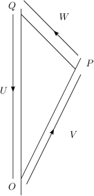
Figure 4: Schematic structure of the $H$-term in $r$, Eq. (46). Notation follows Eqs. (46)–(49).

Figure 5: Schematic structure of the $J$-term in $r$, Eq. (47). Notation follows Eqs. (46)–(49).

V.2.3 Time delay and gauge invariance

As proven in Theorem 1, the time delay is a gauge-invariant observable. From the formula

$$\tau(s)=\tilde{t}=e^{\tilde{r}}\tau_{\mathrm{cl}}(s)=\tau_{\mathrm{cl}}(s)+r\tau_{\mathrm{cl}}(s)+\mathcal{O}(h^{2}),$$ (50)

that relates the linearized gravity correction $r\tau(s)$, Eq. (44), to the Minkowski space result $\tau_{\mathrm{cl}}(s)$, Eq. (20), it is obvious that $r$ should be invariant under linearized gauge transformations. This can be checked explicitly using the gauge transformation formulas, Eqs. (126) and (130), for the terms making up $H_{ij}$ and $J_{i}$. As a consequence, which is given at the bottom of the Appendix, the closure of the $VWU$ triangle in Minkowski space implies the individual gauge invariances of both $H_{ij}$ and $J_{i}$, and hence of $r$.

The last remark deserves some emphasis. There have been many attempts to try to achieve some sort of explicit and complete classification of gauge-invariant observables of general relativity Bergmann (1961); Rovelli (1991); Dittrich (2006); Lusanna and Pauri (2006); Pons et al. (2010). So far, no such complete classification is known. Even in the case of a partial classification, such lists of gauge-invariant observables are often obtained without direct physical interpretation. The strategy of this paper has been different. The idea was to first establish an operational definition of an observable, in terms of the thought experiment described in Sec. II, second to establish a mathematical model thereof, which would naturally be gauge-invariant though perhaps only defined implicitly, and third to use an approximation method (linear-order perturbation theory, in this case) to obtain an explicit expression for the observable. The result of this strategy is an explicit (linearly) gauge-invariant expression for an observable $r$ and a physical interpretation of it as an approximation to the outcome of a clearly described thought experiment. It is of course highly likely that an exhaustive classification of gauge-invariant observables, for the simpler problem of linearized gravity, would have identified explicit expressions like $H_{ij}$ and $J_{i}$, but it is at the same time highly doubtful that they would be accompanied by the clear physical interpretation we have managed to associated to their particular combination in (44).

It is also worth noting that the works of Ford et al. Ford (1995); Yu and Ford (1999); Borgman and Ford (2004); Thompson and Ford (2006) and Roura and Arteaga [13] worked in a particular gauge and with more restricted experiment geometries. Thus they did not obtain the same general gauge-invariant expressions that we have derived here. However, similar expressions, expanded even to quadratic order, were obtained in the work of Tsamis and Woodard Tsamis and Woodard (1992).

VI Sketch of quantum mathematical model

Ideally, to be able to theoretically describe quantum effects, the thought experiment protocol described in Sec. II should be translated into a mathematical model within a quantum theory that encompasses both the gravitational field and the experimental apparatus described in the protocol. A naïve attempt to do this is obstructed by several difficulties: (a) the lack of a uniformly accepted (or at the very least sufficiently general) quantum theory of gravity, (b) the identification of a time observable in quantum mechanics, and (c) the difficulties in modeling measurements in quantum mechanics. Fortunately, we can propose pragmatic solutions to each of these problems, as discussed below.

VI.1 Quantum linearized gravity

While it is true that there is no uniformly accepted theory of quantum gravity, there are some common standards that are expected to be met by the final version of any proposal. One such routine benchmark is the ability to reproduce classical general relativity in the appropriate limit. It is worth noting that under very general circumstances (in the absence of strong curvatures), the dynamics of the gravitational field in general relativity can be very closely approximated by the dynamics of linearized gravity, also known as the theory of (linear) gravitational waves. Our experience to date overwhelmingly demonstrates that the quantum theory of any field whose dynamics may be approximated by a linear theory, be it a “fundamental” field as in elementary particle physics or an “effective” field as in condensed matter theory, is well-approximated by the Fock quantization of the approximate linear theory. By inductive reasoning, we presume that any proposed theory of quantum gravity should also be benchmarked by its ability to reproduce quantum linearized gravity. Therefore, pragmatically, we restrict ourselves to the Fock quantization of the linearized gravity field on Minkowski space as the approximate quantum theory of gravity for the purposes of the mathematical model of the time delay observable.

VI.2 Time in quantum mechanics

It is often repeated physics lore that there is no observable in quantum mechanics corresponding to time, which naturally leads one to wonder whether it is even possible to model time measurements in quantum mechanics. This argument is originally due to Pauli (p.63, footnote 2 of Pauli (1980)). Fortunately, when precisely stated, it is much less restrictive than one is first lead to believe Hilgevoord (2002); Muga and Leavens (2000); Olkhovsky (2009); Brunetti et al. (2010). The crux of this argument is a contradiction that stems from the following hypotheses. Suppose we have a quantum mechanical system with Hamiltonian $\hat{H}$, whose spectrum is bounded from below, and an operator observable $\hat{T}$, whose commutation relation with $\hat{H}$ is precisely of the form $[\hat{T},\hat{H}]=i\hbar$, as would be appropriate for a “time observable” $\hat{T}$ (together with appropriate continuity and functional analytical conditions). Then, an appeal to the Stone-von Neumann uniqueness theorem (Theorem VIII.14 in Reed and Simon (1981)) establishes a contradiction, as, according to the theorem, both $\hat{T}$ and $\hat{H}$ must have continuous unbounded spectra. Thus, there cannot exist such an observable $\hat{T}$ corresponding to time. However, there are at least two physically reasonable ways to circumvent this conclusion. One is to drop the hypothesis that $\hat{H}$ is bounded from below. While this requirement is important for the global, long-term stability of physical systems, its not necessary in some approximate descriptions meant to describe the dynamics of some system for bounded time intervals. Two common examples are a particle in a linear potential and a harmonic oscillator with an inverted potential. The other is to relax the commutation relation condition to $[\hat{T},\hat{H}]\approx i\hbar$, where the correction terms that restore equality may be higher order in $\hbar$ or may be small in another way when restricted to a physically relevant subspace of possible states. An example is a particle on a circle, whose dynamics dictate uniform motion, so that its position can serve as an approximate “cyclic time” observable, like the position of the hand of an analog clock. Many more examples are discussed in Hilgevoord (2002); Muga and Leavens (2000); Olkhovsky (2009) and the references therein.

VI.3 Modeling quantum measurements

VI.3.1 Classical vs quantum measurements

The remaining obstacle is overcome by constructing a fairly explicit, though still rough, model of a measurement, where the system of interest (gravitational field, lab, probe, signal), the measurement devices (proper time clocks) and recording devices are all taken into account. The details of this setup are described below, following some of the ideas of Page and Wootters (1983); Gambini et al. (2009) on the use of physical clocks in quantum systems. The conclusion can be formulated as follows. After the reception and emission times of a signal have been measured by the lab and individually stored, the states and the dynamics of the storage devices stabilize and decouple from the rest of the system, as well as from each other, in the asymptotic future. Then, in the asymptotic future, the corresponding “readout” observables $\hat{S}$ (recorded reception time) and $\hat{T}$ (recorded emission time) commute and thus define a joint (classical) probability distribution $\rho(\sigma,t)=\langle\delta(\hat{S}-\sigma)\delta(\hat{T}-t)\rangle$, where the expectation value is taken with respect to the (Heisenberg) state of the total system, which we will refer to as the quantum gravitational vacuum. Mathematically, this probability distribution $\rho(\sigma,t)$ may be referred to as either the joint spectral density of the quantum gravitational vacuum with respect to the operators $\hat{S}$ and $\hat{T}$. In more physical terms, $\rho(\sigma,t)$ is the absolute value squared of the wave function of the quantum gravitational vacuum projected onto the variables $\sigma$ and $t$.

Recall that the main output the classical mathematical model of the measurement of the time delay observable is the functional relation $t=\tau(s)$, which can be seen as a special case of a joint probability distribution $\rho_{\mathrm{cl}}(\sigma,t)=\delta(\sigma-s)\delta(t-\tau(\sigma))$, where $s$ is the predetermined time when the laboratory makes the measurements. This classical probability distribution is so “sharp” because we take as a classical state a definite configuration of the gravitational field. More generally, in the framework of classical statistical mechanics, we can take any probability measure $d\rho(g)$ on the space of gauge equivalence classes of the configurations of lab-equipped spacetimes. The main output of the classical mathematical model of the time delay measurement in this state is then the probability distribution $\rho_{\mathrm{cl}}(\sigma,t)=\int d\rho(g)\,\delta(\sigma-s)\delta(t-\tau_{g}(\sigma))$, where the dependence of the emission time $\tau_{g}(s)$ on the equivalence class $g$ of lab-equipped spacetime configurations is indicated through a subscript. Thus, considering quantum mechanics as an extension (or rather deformation) of classical statistical mechanics, it is not surprising that the main output of a quantum mathematical model of a measurement of the time delay observable is the probability distribution $\rho(\sigma,t)$. Of course, being the result of a quantum measurement, the distribution $\rho(\sigma,t)$ depends on more details of the measurement (such as the order in which the measurements were carried out) than the classical distribution $\rho_{\mathrm{cl}}(\sigma,t)$.

VI.3.2 Dynamical apparatus model

The full system included in the model consists of the following dynamical subsystems: the gravitational field $\hat{g}$, the lab and probe worldline coordinates $\hat{y}_{l}$ and $\hat{y}_{p}$, the lab and probe proper time clocks $\hat{\tau}_{l}$ and $\hat{\tau}_{p}$, the time registers $\hat{S}$ and $\hat{T}$ in the lab, the coordinates of the signal particles $\hat{z}$, and the time stamp $\hat{\tilde{\tau}}$ carried by each signal particle. The spacetime is presumed to have a fixed foliation by level sets of a time function $t$. The gravitational field is taken to be completely gauge fixed, for instance using the transverse, traceless, and $t$-compatible radiation conditions (Sec. 4.4b of Wald (1984)). All worldlines can then be parametrized by $t$ as well. The dynamics of the full system, describing its evolution with respect to time $t$, is specified by a Hamiltonian

$$\hat{H}=\hat{H}_{\mathrm{sub}}+\hat{H}_{\mathrm{geom}}+\hat{H}_{\mathrm{meas}},$$ (51)

which is composed of $\hat{H}_{\mathrm{sub}}$ describing the independent dynamics of the subsystems, of $\hat{H}_{\mathrm{geom}}$ describing the necessary interactions or external interventions to effect the geometry of the experimental setup, and of $\hat{H}_{\mathrm{meas}}$ describing the coupling between the recording devices and the rest of the system during the measurement.

Since we are mostly concerned here with a quantum model of measurement of the clock readings, we will concentrate only on $\hat{H}_{\mathrm{meas}}$ and specify $\hat{H}_{\mathrm{sub}}$ and $\hat{H}_{\mathrm{geom}}$ mostly verbally.

The dynamics of the gravitational field follow the appropriate gauge fixed Hamiltonian, a term in $\hat{H}_{\mathrm{sub}}$ derived from the Einstein-Hilbert action. The precise details of the implementation of this idea are irrelevant for this discussion, as long as the corresponding dynamics about the quantum gravitational vacuum can be approximated by the dynamics of linearized gravity about the Fock vacuum. This assumption is the basis of the calculation sketched in Sec. VII.

The worldlines of various particles are described by their spatial coordinates as functions of the global time $t$, $\hat{y}^{i}_{l}(t)$, $\hat{y}^{i}_{p}(t)$, and $\hat{z}^{i}(t)$. The dynamics of these variables follow from the appropriate terms in $\hat{H}_{\mathrm{sub}}$. The lab and probe worldlines are timelike geodesics, with an appropriate term in $\hat{H}_{\mathrm{geom}}$ providing a kick to the probe at event $O$ to give it a fixed relative velocity with respect to the lab. (The fact that $O$ lies on the lab worldline can be used as one of the gauge-fixing conditions.) To imitate the action of a continuously emitted signal field (like the electromagnetic field), the multiplicity of signal particles are indexed by a time $t^{\prime}$ and a unit $3$-vector $\mathbf{n}$. The dynamics as specified by terms in $\hat{H}_{\mathrm{sub}}$ and $\hat{H}_{\mathrm{geom}}$ should be as follows. The worldline $\hat{z}^{i}_{(t^{\prime},\mathbf{n})}(t)$ follows the probe worldline until the time $t=t^{\prime}$, after which point the worldline of $\hat{z}^{i}_{(t^{\prime},\mathbf{n})}(t)$ becomes null with direction determined by $\mathbf{n}$. (This is a kind of eikonal approximation, which replaces a massless field by a large collection of massless particles.) The initial state of each of these particles is presumed to be of a localized wave packet form, with negligible wave packet spread on time scales comparable to the geometry of the experiment.

There are two potential problems in constructing a detailed quantum model implementing the above requirements. While it is not difficult to write down a classical version of such $\hat{H}_{\mathrm{sub}}+\hat{H}_{\mathrm{geom}}$, the generalization to quantum mechanics is not unique, due to the usual operator ordering ambiguities. The standard solution of this problem is to parametrize these ambiguities and realize that different choices of these parameters correspond to physically different models. Thus, the fixation of these parameters must be part of the full specification of the detailed model. Fortunately, these ordering ambiguities are generically expected to be suppressed by powers of $\hbar$. Moreover, we assume that their parametrization may be tuned to maximize the validity of the approximations used in Sec. VII. The second problem is that coupling point particles to fields generically leads to singular dynamics. (The singularities inherent in the naive interaction of a classical point electron with its own electromagnetic field is a classical example of this difficulty.) However, this issue can be dealt with straightforwardly by spatial smearing of the particle-metric field interaction terms. The spatial extent of the smearing becomes another parameter whose value is to be chosen as to minimize the impact of the smearing on the rest of the discussion. Alternatively, the interaction term could be modified in a more sophisticated way, without introducing non-local smearing, for instance along the lines suggested by the recent work on classical point particles coupled to their self-force Poisson et al. (2011) or by appealing to intrinsic quantum uncertainty of the center of mass coordinates as in Göklü et al. (2009).

The state spaces for the clock and time register subsystems can be presumed to be completely internal (i.e., divorced from spacetime coordinates) and thus can be subject to even further simplifications. The time register subsystems $\hat{S}$, $\hat{T}$ and $\hat{\tilde{\tau}}_{(t^{\prime},\mathbf{n})}$ should be very stable, thus their contribution to $\hat{H}_{\mathrm{sub}}$ should be approximately zero. On the other hand, the clock variables $\hat{\tau}_{l}(t)$ and $\hat{\tau}_{p}(t)$ should evolve approximately monotonically, with rates set by their local proper time. This can be accomplished by a contribution to $\hat{H}_{\mathrm{sub}}$ of the form $\dot{\hat{\tau}}_{l}\hat{P}_{\tau_{l}}+\dot{\hat{\tau}}_{p}\hat{P}_{\tau_{p}}$, where $\hat{P}_{\tau_{l}}$ and $\hat{P}_{\tau_{p}}$ are respectively canonically conjugate to $\hat{\tau}_{l}$ and $\hat{\tau}_{p}$, while $\dot{\hat{\tau}}_{l}$ and $\dot{\hat{\tau}}_{p}$ stand for the appropriate expressions in terms of $\dot{\hat{y}}^{i}_{l}$, $\dot{\hat{y}}^{i}_{p}$ and $\hat{g}$. Note that this choice of Hamiltonian circumvents Pauli’s impossibility argument by virtue of being unbounded from below.

Finally, $\hat{H}_{\mathrm{meas}}$ is chosen to implement the idea of weak measurement Braginsky and Khalili (1995). The idea of weak measurement can be described as follows. Suppose there is a quantum variable $\hat{q}$ whose value we wish to measure and record in another variable $\hat{Q}$, belonging to a recording device subsystem. Suppose that $\hat{P}$ is canonically conjugate to $\hat{Q}$ and that $\hat{Q}$ suffers negligible evolution on its own. Then the value of $\hat{Q}$ can be measured at any convenient time after the weak measurement took place, thus allowing us to infer (subject to quantum uncertainties) the value of $\hat{q}$ at the time of measurement. The measurement itself can be modeled using the interaction Hamiltonian $f_{\mathrm{trig}}(t)\hat{q}\hat{P}$, where $f_{\mathrm{trig}}(t)$ is a trigger factor, which is non-zero only during the time interval when the measurement is supposed to take place. The operators $\hat{q}(t)$ and $\hat{P}(t)$ are presumed to commute at equal times, as they belong to independent subsystems, so their ordering of the interaction Hamiltonian is unambiguous. If this interval is of length $\Delta t$ and during it $f_{\mathrm{trig}}(t)\approx f_{0}$ is approximately constant, we can see that this interaction Hamiltonian effects the evolution

$$Q_{\mathrm{after}} =e^{i\int\mathrm{d}{t}\,f_{\mathrm{trig}}(t)qP}Q_{\mathrm{before}}e^{-i\int\mathrm{d}{t}\,f_{\mathrm{trig}}(t)qP}$$ (52)

$$=Q_{\mathrm{before}}+\int\mathrm{d}{t}\,f_{\mathrm{trig}}(t)q$$ (53)

$$\approx Q_{\mathrm{before}}+\Delta tf_{0}q(t_{0}),$$ (54)

where the last approximation holds provided $t_{0}$ was part of the measurement time interval and $\hat{q}(t)$ and $\hat{P}(t)$ evolved negligibly during it. In general, the trigger $f_{\mathrm{trig}}$ need not be a scalar, and may itself be a operator that commutes with both $\hat{q}(t)$ and $\hat{P}(t)$. Also while each pair of factors commutes at equal times, in general, they will not commute at unequal times (even with themselves). Thus, the evolution effected by the interaction will involve the time-ordered exponential of the interaction Hamiltonian and will look more complicated than Eq. (52). However if the interaction Hamiltonian can be considered as a small perturbation, then at linear order $\hat{Q}_{\mathrm{after}}$ will look the same as Eq. (54).

With the above discussion in mind, we set the measurement interaction Hamiltonian to

$$\hat{H}_{\mathrm{meas}}=\delta[\hat{\tau}_{l}-s]\dot{\hat{\tau}}_{l}\\ {}\times\left[\hat{\tau}_{l}\hat{P}_{S}+\int\mathrm{d}{t^{\prime}}\mathrm{d}{\mathbf{n}}\,\delta^{3}[\hat{z}_{(t^{\prime},\mathbf{n})}-\hat{y}_{l}]\hat{\tilde{\tau}}_{(t^{\prime},\mathbf{n})}\hat{P}_{T}\right].$$ (55)

Note that the factors in each product commute at equal times (recall that $\dot{\hat{\tau}}_{l}$ is not canonically conjugate to $\hat{\tau}_{l}$), so their ordering in $\hat{H}_{\mathrm{meas}}$ is unambiguous. The extra factor of $\dot{\hat{\tau}}_{l}(t)$ is there to ensure that $\hat{H}_{\mathrm{meas}}$ is defined independent of the choice of the background time $t$. Under the hypotheses explained in the previous paragraph, the asymptotic future values of $\hat{S}$ and $\hat{T}$ operators can be approximated as

$$\hat{S}^{+} =\lim_{t\to\infty}\hat{S}(t)$$ (56)

$$\approx\hat{S}_{\mathrm{before}}+\int\mathrm{d}{t}\,\delta[\hat{\tau}_{l}(t)-s]\dot{\hat{\tau}}_{l}(t)\hat{\tau}_{l}(t)$$ (57)

$$T^{+} =\lim_{t\to\infty}\hat{T}(t)$$ (58)

$$\approx\hat{T}_{\mathrm{before}}+\int\mathrm{d}{t}\,\delta[\hat{\tau}_{l}(t)-s]\dot{\hat{\tau}}_{l}(t),$$ (59)

$$\qquad{}\times\int\mathrm{d}{t^{\prime}}\mathrm{d}\mathbf{n}\,\delta^{3}[\hat{z}_{(t^{\prime},\mathbf{n})}(t)-\hat{y}_{l}(t)]\hat{\tilde{\tau}}_{(t^{\prime},\mathbf{n})}(t).$$

Provided $\hat{S}_{\mathrm{before}}$ and $\hat{T}_{\mathrm{before}}$ have zero expectation value, the measurements of $\hat{S}^{+}$ and $\hat{T}^{-}$ the above asymptotic limits provide unbiased estimates of the remaining terms, which can be interpreted respectively as the reception and emission times defined in the time delay experimental protocol.

We conclude this analysis by noting that, provided that any potential uncertainties can be neglected or modeled and subtracted, it is reasonable to assume that the spectral density of the quantum gravitational vacuum with respect to $\hat{S}$ can be well-approximated by

$$\langle\delta(\hat{S}^{+}-\sigma)\rangle\approx\delta(\sigma-s).$$ (60)

It follows that it is then also reasonable to assume that the joint spectral density of the quantum gravitational vacuum with respect to $\hat{S}^{+}$ and $\hat{T}^{+}$ will be well-approximated by

$$\rho(\sigma,t)=\langle\delta(\hat{S}^{+}-\sigma)\delta(\hat{T}^{+}-t)\rangle\approx\delta(\sigma-s)\rho_{s}(t).$$ (61)

The probability distribution $\rho_{s}(t)$ then has the interpretation of the spectral density of the quantum gravitational vacuum with respect to the quantum emission time operator observable $\hat{\tau}(s)$, where the quantum emission time observable can then be identified as $\hat{\tau}(s)=\hat{T}^{+}$. The quantum time delay observable is then simply $\delta\hat{\tau}(s)=s-\hat{\tau}(s)$.

At this point it is worth considering a bit more precisely how the probability distributions of Eqs. (60) and (61) relate to those that would be obtained by a physically realized experiment following the same operational protocol. Above, we have explicitly stated that these expressions are expected to be applicable provided all sources of quantum (or classical) fluctuations other than the quantum gravitational vacuum are neglected. How can this neglect be reasonable? These neglected sources are numerous, as for instance discussed in the later Sec. VII.3. Moreover, by now, the study of uncertainties in measurements of space and time intervals induced by quantum fluctuations of the internal states of a measurement apparatus is classical subject, going back to a seminal paper of Salecker and Wigner Salecker and Wigner (1958). These effects can be quite large compared to the Planck-scale effects (Sec. VII.4) that we are concerned with here.

The main difference between the effects we neglect and the effect that we actually study is that the former depend primarily on the internal physics of the apparatus, while the latter depends crucially on the dynamical quantum gravitational field. That is, the effect that we study is genuinely due to quantum gravity, while those we neglect are not. If we are concerned with a question of principle, which is to account for all possible sources contributing to the variance of the time delay or time emission observables described earlier, it is not sufficient to include only the internal apparatus sources or only the quantum gravitational effects (independent of their relative size), it is in fact necessary to consider both of them. The internal apparatus fluctuation sources have already been studied extensively in the literature spawned by the original work Salecker and Wigner (1958). On the other hand, genuine quantum gravitational effects have received much less attention (a review of the relevant literature was given in the Introduction) and are hence the main focus of the current work. Since these contributions to the observational variance are separate, they can be analyzed separately and, at the leading perturbative order, contribute essentially additively.

When restored, the effects of quantum fluctuations of the internal dynamics of the clocks and recording devices used in described measurement models replace the sharp $\delta$-function in Eq. (60), as well as in the analogous equation for $\hat{T}^{+}$, by a broader probability distribution $\rho_{\text{int}}(\sigma-s)$. The joint probability distribution (61) would also be broadened broadened by convolution with $\rho_{\text{int}}$ in both the $\sigma$ and $t$ arguments.

Finally, the calculations outlined in this paper do more than answer a question of principle. As previously mentioned, they serve as a toy model for resolving the challenges inherent in the problem of observables in quantum gravity. So the lessons learned here, may be applicable to a situation like early Universe cosmology, which is a more likely source of physically measurable quantum gravitational effects Woodard (2009).

VII Sketch of calculation in quantum linearized gravity

The point of the preceding section was to motivate that the output of an explicit quantum calculation should be a probability distribution $\rho_{s}(t)$, which should be interpreted as the spectral density of the time register $\hat{T}$ with respect to the quantum gravitational vacuum (projected onto the $s$-eigensubspace of the time register $\hat{S}$). Phenomenologically, dropping the subscript $s$ since no other probability distribution would be considered from now on, $\rho(t)$ should be interpreted as the statistical distribution of measurement outcomes for an ensemble of repeated measurements of the emission time $\hat{\tau}(s)$ (reproducing the geometry of the experiment for each repetition). Again, motivated by the discussion of the preceding section, we propose that, within the linearized gravity approximation and keeping all available parameters tuned to minimize all influences on the measurement of emission time other than the effects of the gravitational field, the role of the observable $\hat{T}$ should be played by the linearized expression (50) with the classical graviton field everywhere replaced by the quantized graviton field (with one caveat to be discussed below) and the role of the quantum gravitational vacuum should be played by the Poincaré-invariant Fock vacuum of the graviton field. Within this proposal, the probability distribution $\rho(t)$ can be computed explicitly. We leave the details of this calculation to be presented elsewhere  and only discuss some general aspects of it that can be deduced from dimensional analysis and the nature of perturbative calculations.

VII.1 Gaussian spectral density

In linearized gravity on Minkowski space, we interpret the Poincaré-invariant Fock vacuum $|0\rangle$ as the quantum gravitational vacuum and the operator $\hat{\tau}(s)$ as the quantum emission time. From the preceding discussion, our goal is to evaluate the spectral density $\rho(t)$ of $|0\rangle$ with respect to $\hat{\tau}(s)$. This simplified problem has an explicit solution. A linear field theory is essentially a collection of harmonic oscillators and, by construction, the Fock vacuum is a Gaussian state (with zero mean) with respect to the oscillator variables. In other words, the Fock vacuum is also Gaussian with respect to any observable linear in the graviton field $\hat{h}(x)$, such as $\hat{\tau}(s)$. Therefore, the sought probability distribution $\rho(t)$ is Gaussian. It is fully determined by its mean, which is just the classical Minkowski space expression (20), and its variance, which can be obtained from the expectation value $\langle 0|\hat{\tau}(s)^{2}|0\rangle$.

It is clear that the calculation of the probability distribution $\rho(t)$ is reduced to evaluating a single vacuum expectation value given above. Recall that the emission time is invariant with respect to gauge transformations that fix the synchronization point $O$ and the lab tetrad frame at it. However, due to the Poincaré invariance of the Fock vacuum, the expectation value $\langle 0|\hat{\tau}(s)^{2}|0\rangle$, which combines the observable and the state, is actually invariant under arbitrary gauge transformations and no longer depends on the special choice of synchronization point or lab tetrad frame.

VII.2 Causal inequalities and perturbation theory

In Sec. IV, we found that the time delay and emission time observables obey some causal inequalities. The validity of these inequalities relies mainly on the Lorentzian character of the metric tensor and the geodesic character of inertial motion. Therefore, classically, violations of these inequalities would be evidence of superluminal signal propagation or violation of the equivalence principle. Thus we can naturally take the following objective criterion for the presence of causality violation in quantum theory: violation of causal inequalities by the spectral density of the quantum gravitational with respect to the time delay observable.

Quantum theory is famous for tunneling phenomena. For example, a quantum state may be such that a measurement may find a particle (though likely with only small probability) in a region that is classically forbidden to it. Similarly, we would like to investigate whether the causal inequalities are strictly obeyed in the quantum theory or are subject to violations via “quantum tunneling.” A definite answer to this question would go a long way toward informing the debate on whether any quantum theory of gravity necessarily entails causality violations Wheeler (1962); Kent (2009). While it would be very difficult to settle this debate, in large part due to the breadth of the subject matter, as stated. However, an explicit example of a quantum gravitational theory without causality violation would force a weakening of the “necessarily entails” clause. Equally, a fairly conservative (no extra matter, no extra dimensions, no causality violation in the classical limit, though taken only in a linear approximation) example of a quantum gravitational model with causality violation would strengthen the evidence for the “any” clause.

Unfortunately, as should become immediately obvious, the perturbative calculations outlined in this section are not conclusive enough to establish whether causality violation actually takes place or not. In short, since the spectral density is expected to be Gaussian (as discussed in Sec. VI),

$$\rho(t)\sim\exp\left(-\frac{(t-\tau_{\mathrm{cl}})^{2}}{2(\Delta\tau)^{2}}\right),$$ (62)

with some mean $\tau_{\mathrm{cl}}$ and variance $(\Delta\tau)^{2}$, all real values of $t$ acquire a non-zero probability of being measured. Thus, the causal bounds on $t$ are clearly violated, as illustrated in Fig. 6. However, the responsibility for this violation can be ultimately traced back to the perturbative approximation rather than to the quantum theory. Recall that classically, as discussed in Sec. IV, the proofs of these causal bounds crucially relied on the Lorentzian character of the metric, as well as on the detailed behavior of geodesics in Lorentzian spacetimes. Neither of these properties survives in perturbation theory. One can find classical field configurations of $h_{ij}(x)$ for which the linearized classical expression for $\tau(s)$ violates the causal inequalities as well. For these field configurations $h_{ij}(x)$ would have to be of the same order as the background metric $\eta$, which is precisely the regime where perturbation theory is no longer applicable.

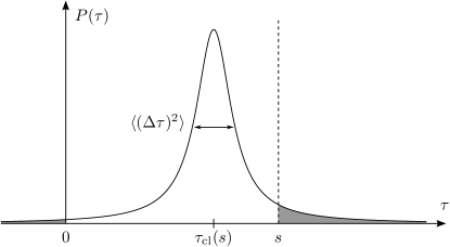
Figure 6: Spectral density of the linearized quantum gravitational vacuum with respect to the emission time $\tau(s)$. In a linear field theory, the spectral density is expected to be Gaussian, with mean $\tau_{\mathrm{cl}}(s)$ and variance $\langle(\Delta\tau)^{2}\rangle$. The mean is the emission time in Minkowski space, Eq. (20). This probability distribution clearly penetrates the shaded region, which is forbidden by classical causal inequalities.

In conclusion, the perturbatively calculated $\rho(t)$ may be presumed to give accurate results around the interval $[\tau_{\mathrm{cl}}-\Delta\tau,\tau_{\mathrm{cl}}+\Delta\tau]$, but not for larger or smaller values. Unfortunately, the information needed to decide whether causal inequalities are actually violated requires the knowledge of $\rho(t)$ precisely in the regions where the perturbative approximation is no longer expected to be valid.

VII.3 Finite measurement resolution

The detailed calculation of the vacuum fluctuation of $\hat{\tau}(s)$ immediately presents a problem: it is infinite. This infinity can be traced back to the singularity of the two-point function

$$G(x-y)=\langle\hat{h}(x)\hat{h}(y)\rangle\sim\frac{1}{(x-y)^{2}}$$ (63)

in the coincidence limit $x\to y$. This infinity has a straightforward physical interpretation, which at the same time suggests a meaningful regularization of the divergence.

Any realistic measurement of the quantum field $\hat{h}(x)$ is carried out by a detector with finite spatial and temporal resolution. Thus, no measurement is ever sensitive directly to the field evaluated at a single spacetime point $x$, rather measurements are typically sensitive to smeared fields Bohr and Rosenfeld (1950); Bergmann and Smith (1982)

$$\tilde{h}(x)=\langle\!\langle\hat{h}(x-z)\rangle\!\rangle=\int\mathrm{d}{z}\,\hat{h}(x-z)g(z),$$ (64)

where $g(z)$ is a smooth test function peaked in the neighborhood of $0$, and $\langle\!\langle{\cdots}\rangle\!\rangle$ denotes the smearing with respect to $g(z)$. The smearing function $g(z)$ may be interpreted as the detector sensitivity profile, which clearly depends on how the measurement was carried out. The vacuum fluctuation of the smeared field at $x$ is then always finite

$$\langle\tilde{h}(x)^{2}\rangle =\int\mathrm{d}{z_{1}}\mathrm{d}{z_{2}}\,G(x-z_{1}+z_{2})g(z_{1})g(z_{2})$$ (65)

$$=\int\mathrm{d}{z}\,G(x-z)\tilde{g}(z)$$ (66)

$$\sim\langle\!\langle\frac{1}{(x-z)^{2}}\rangle\!\rangle$$ (67)

$$\sim\frac{1}{\mu^{2}},$$ (68)

where $\tilde{g}(z)=(g*g)(z)$ is the convolution of $g(z)$ with itself, by abuse of notation $\langle\!\langle{\cdots}\rangle\!\rangle$ also denotes smearing with respect to $\tilde{g}(z)$, and $\mu$ is the length scale over which $g(z)$ has appreciable support, which is the spatiotemporal resolution of the detector. Physically, this estimate means that the root-mean-square noise in a detector, due to quantum fluctuations, grows as inversely proportional to its resolution (Bohr and Rosenfeld (1950) and Secs. 10.9.1–2 of Mandel and Wolf (1995)). Such fluctuations are vividly illustrated in the context of quantum optics in Fig. 2.1 of Leonhardt (1997).

Since we are working with an idealized model of physical measurement, it is natural that the quantum fields entering into the expression for the emission time $\hat{\tau}(s)$ should be smeared. Unfortunately, the details of precisely how the smearing is to be done are quite complicated. They in general depend on all the aspects of the experiment: the resolutions of the proper time clocks, the coupling of the lab and probe centers of mass to the gravitational field in geodesic motion, sharpness of the signals transmitted by the probe, etc. For the purposes of this discussion, we do not need such detailed information, as for simplicity we would only be interested in the asymptotic limit of perfect detector resolution $\mu\to 0$. This limit is obviously divergent, so we can settle for the leading term in an expansion in inverse powers of $\mu$. Therefore, we simply assume that all occurrences of the point field $\hat{h}_{ij}(x)$ are replaced by the smeared field $\tilde{h}(x)$, Eq. (64). That is, the smearing function $g(z)$ is the same everywhere, independent of $x$. The only thing we assume about $g(z)$ is that it is regular enough to render the vacuum fluctuation of $\hat{\tau}(s)$ finite and that it is peaked only at the origin, with appreciable support over a region of size $\mu$, so that we can estimate its moments as

$$\langle\!\langle z^{k}\rangle\!\rangle\sim\mu^{k},$$ (69)

where $z^{k}$ represents any homogeneous expression of order $k$ in the components of $z$. It is worth noting that, as stated, this smearing convention breaks background Lorentz invariance. This is clearly unphysical. Nevertheless, we make this assumption in the current and some future calculations for the purposes of working out their general structure. A more physical smearing convention should be re-examined in the future alongside with more realistic models of lab, probe, and signal subsystems.

It is worth noting at this point that the works of Ford et al. Ford (1995); Yu and Ford (1999); Borgman and Ford (2004); Thompson and Ford (2006) took a completely different approach to the regularization of divergences arising from the singularities of the graviton two-point function. In particular, they treated several scenarios that produced fluctuations different from Minkowski space (finite temperature state, squeezed vacuum, extra compactified dimensions), which were regularized by subtracting the divergent Minkowski, Poincaré-invariant vacuum result. Thus these previous calculations computed the deviation of the quantum fluctuations from that of Minkowski space, but did not directly address Minkowski space results themselves, unlike we do in this work.

VII.4 Dimensional analysis

Looking at the structure of the explicit expression for the linearized correction $r\tau_{\mathrm{cl}}(s)$ to the emission $\tau(s)$, Eq. (50), it is fairly obvious that a detailed calculation of the variance $\langle\tilde{r}^{2}\rangle$ of the smeared correction $\tilde{r}$, where each occurrence of the classical field $h(x)$ is simply replaced by the smeared quantum field $\tilde{h}(x)$, will be quite involved. The expression for $r$, whose structure is illustrated at the end of Sec. (V.2.2), contains on the order of $10$ terms. Therefore, the number of terms in $\tilde{r}^{2}$ will be of order $100$. Each of these terms consists of two (possibly iterated) integrals over spacetime segments over (possibly iterated) derivatives of the smeared $\langle\!\langle G(z)\rangle\!\rangle$ graviton two-point function. The total number of nested integrations for each term is five (5), which includes two (2) from the spacetime segment and three (3) from smearing. Using symmetry, one or two integrations may be made trivial. However, it is unavoidable that each of the order $100$ is a high-dimensional integral. Moreover, the integrands are distributions, rather than continuous functions, whose singularities are ultimately traceable to the light-cone and coincidence singularities of the graviton two-point functions. The high dimensionality of the integrals and the distributional character of the integrands makes it very difficult to treat them numerically. On the other hand, the integrands of these order $100$ terms may have many different algebraic structures, preventing the evaluation of a single master analytical expression that could be uniformly applied to all of them. Splitting each term into simpler pieces and considering all possible cases of algebraic structures easily leads to thousands of individual integrals to be evaluated analytically. There is little choice but to resort to hybrid numerical-analytical calculations automated using computer algebra software. These detailed calculations are in progress and their results will be reported elsewhere [32]. In the rest of this section we concentrate on some intermediate, qualitative results that may be obtained by straightforward dimensional analysis.

Taking dimensionful constants into account, and keeping in mind that the field $h(x)$ is itself dimensionless, the unsmeared graviton two-point functions has the form

$$\langle\hat{h}(x)\hat{h}(y)\rangle=G(x-y)\sim\frac{\ell_{p}^{2}}{(x-y)^{2}},$$ (70)

where the denominator of the last expression is the spacetime interval squared, $(x-y)^{2}=\eta_{ij}(x-y)^{i}(x-y)^{j}$, and the numerator is the Planck length squared, $\ell_{p}^{2}=G\hbar/c^{3}$. What is important here is that $G(z)/\ell_{p}^{2}\sim 1/z^{2}$ is a homogeneous function of $z$ of degree $-2$ and hence of length dimension $[G(z)/\ell_{p}^{2}]=-2$. The scales $\mu$ and $\ell_{p}$ and the components of $z$ itself all have length dimension $[z]=[\mu]=[\ell_{p}]=1$. On the other hand, a derivative with respect to $z$ has length dimension $[\nabla]=-1$. Generically it has the effect $\nabla z^{n}\sim z^{n-1}$. Using the convention from the Appendix, the spacetime segment integrals are all affinely parametrized from $0$ to $1$ and hence are dimensionless, $[\int_{X}]=0$. On the other hand, integration over a spacetime segment has the generic effect $\int_{X}z^{n}\sim z^{n+1}/s$, where $s$ is the length scale of the segment $X$, $[s]=1$, and $z$ on the right hand side corresponds to the coordinates of the segment’s end points.

Without smearing, the expectation value $\langle r^{2}\rangle$ is infinite. Smearing introduces a regulating length scale $\mu$, the detector resolution. Therefore, the smeared expectation value $\langle\tilde{r}^{2}\rangle$ should diverge as $\mu\to 0$. The details of the approach of $\mu$ to $0$ in general depend on the details of the smearing functions. Fortunately, a kind of universality among all well-behaved localized smearing functions can be obtained by concentrating on the leading terms in an expansion of the result in inverse powers of $\mu$.

From the structure of the explicit expression for $r$, keeping in mind that derivatives worsen singularities while integrals improve them, the most singular contribution should come from the terms with the greatest number of derivatives and the least number of integrals. Namely, $r\sim r_{X}\int_{X}\nabla h$, where $r_{X}$ is some tensorial coefficient dependent on the geometry of the segment $X$. Note that, since both $r$ and $h$ are dimensionless, the tensorial coefficient $r_{X}$ must have length dimension $[r_{X}]=1$ and be of order $s$ in magnitude, due to the standard affine parametrization of the integral over $X$. In fact, it should be of size $s$, which is the length scale of the spacetime segment $X$. The leading-order contribution to the smeared variance of $r$ can then be estimated as follows:

$$\langle\tilde{r}^{2}\rangle \sim\left\langle\left(\sum_{X}r_{X}\int_{X}\nabla\tilde{h}\right)^{2}\right\rangle$$ (71)

$$\sim s^{2}\langle\!\langle\int_{X}\int_{Y}\nabla^{2}G(z)\rangle\!\rangle$$ (72)

$$\sim s^{2}\langle\!\langle\int_{X}\int_{Y}\nabla^{2}\frac{\ell_{p}^{2}}{z^{2}}\rangle\!\rangle$$ (73)

$$\sim s^{2}\langle\!\langle\int_{X}\int_{Y}\frac{\ell_{p}^{2}}{z^{4}}\rangle\!\rangle$$ (74)

$$\sim s^{2}\langle\!\langle\frac{\ell_{p}^{2}}{s^{2}z^{2}}\rangle\!\rangle\sim\langle\!\langle\frac{\ell_{p}^{2}}{z^{2}}\rangle\!\rangle\sim\frac{\ell_{p}^{2}}{\mu^{2}}$$ (75)

Detailed calculations show that many terms do have this scaling behavior, but also that terms of the form $(\ell_{p}^{2}/\mu^{2})\log(\mu/s)$ and $(\ell_{p}^{2}/\mu^{2})(s/\mu)$ show up at intermediate stages as well. While the appearance of logarithmic scaling is not unusual in quantum calculations, the last term is somewhat surprising and, if uncanceled in the final result, may cast serious doubt on the validity of the linearized approximation in the regimes of very large $s/\mu$ ratios. This ratio corresponds to that of the spatial and temporal extent of the experiment to the resolution of the detectors involved.

From Eq. (50), the perturbative correction to the emission time $\tau(s)$ and the time delay $\delta\tau(s)$ scale like $sr$, and so the quantum variances of $\hat{\tau}(s)$ and $\delta\hat{\tau}(s)$ should scale like $s^{2}\langle\tilde{r}^{2}\rangle$, since $\langle\tilde{r}\rangle=0$. From this and the possible leading-order contributions to the smeared variance of $r$ we can deduce the root-mean-square size of fluctuations expected in observations of the time delay due to the fluctuations of the quantum gravitational vacuum shown in Table 1. Let us contrast two possible experimental contexts. In the laboratory context, the spatiotemporal extent of the experiment (with time-length conversion via the speed of light) is expected to be $s\sim 1~{}\mathrm{m}\sim 10^{-9}~{}\mathrm{s}$, while in the cosmological one $s\sim 1~{}\mathrm{Mpc}$. Recall that a megaparsec is $1~{}\mathrm{Mpc}\sim 10^{22}~{}\mathrm{m}\sim 10^{14}~{}\mathrm{s}$. For the detector resolution scale, we select $\mu\sim 1~{}\mathrm{nm}\sim 10^{-18}~{}\mathrm{s}$. This is of the order of the wavelength of X-rays, which are consistently available in both contexts. The Planck scale as usual is $\ell_{p}\sim 10^{-35}~{}\mathrm{m}\sim 10^{-44}~{}\mathrm{s}$.

Table 1: Estimates for the root-mean-square size of quantum fluctuations in observations of the time delay for different possible leading-order behaviors in $\mu\to 0$.

Context	$s$	$\mu$	$\frac{s\ell_{p}}{\mu}$	$\frac{s\ell_{p}}{\mu}\log(\frac{s}{\mu})^{1/2}$	$\frac{s^{3/2}\ell_{p}}{\mu^{3/2}}$
laboratory	$1$ m	$1$ nm	$10^{-35}$ s	$10^{-34}$ s	$10^{-30}$ s
cosmological	$1$ Mpc	$1$ nm	$10^{-12}$ s	$10^{-11}$ s	$10^{3}$ s

All of the above estimates, except one, are well below the sensitivity or noise thresholds of the current state of the art of experimental and observational technology. So it is not surprising that kind of effect has yet to be observed. Clearly, if the largest of the above estimates were correct, we would have observed this effect long ago due to the very large fluctuations in the arrival times of high frequency photons from distant galaxies. Of course, since that result is only preliminary and comes from the least understood part of intermediate calculations, it has to be taken with a grain of salt. But it does highlight the fact that the linearized approximation employed in the calculations described above may not be valid on large timescales. This is not an unusual feature of perturbation theory. For example, it was noticed long ago in celestial mechanics that there exist perturbative terms that scale with positive powers of time, so-called secular terms, in otherwise non-perturbatively stable systems Giacaglia (1972). This remark also offers some hope that if, in fact, the perturbation expansion in our calculations breaks down on large time scales that this problem could be repaired using the methods already developed for dealing with secular perturbative terms in celestial mechanics or other fields.

VIII Discussion

We have operationally defined a particular physical observable, the time delay $\delta\tau(s)$ [as well as the related emission time $\tau(s)$], and have provided both exact, implicit and approximate, explicit mathematical models for it. The time delay satisfies two important inequalities (stemming from the maximality of light speed and from local geodesic extremality) directly related to the causal structure of classical Lorentzian spacetimes. Thus, it is sensitive to the causal structure of classical dynamical gravity. Moreover, we have sketched how the same operational definition can be used to define a quantum time delay observable and how to compute its variance due to quantum fluctuations of the quantum gravitational vacuum, in linearized gravity, given the usual Fock quantization of the graviton field.

This work opens up many potential lines of investigation. Foremost among them, is the completion of the detailed calculation of the variance of the time delay due to the quantum fluctuations of the quantum gravitational vacuum. That work is in progress and will be reported on elsewhere [32].

An important issue that needs to be explored is the detailed construction of a quantum model of the measurement apparatus sketched in Sec. VI. This model should take into account the quantum dynamics of the center of mass motions of the probe and laboratory, a more detailed representation of the time stamped signal transmitted by the probe, and of the weak measurements of the relevant clock and signal systems. Some existing literature may be helpful in refining these models Göklü et al. (2009); Gambini et al. (2009); Page and Wootters (1983); Braginsky and Khalili (1995).

The triangular geometry of the time delay experiment is one of the simplest possible. However, there is no conceptual obstacle to generalizing the same methodology to more complex geometries, including piecewise geodesic motion with more components and even accelerated motion. It is also natural to capture other effects of the fluctuating gravitational field on the signal, such as angular blurring and other image effects at the reception of the signal by the lab. These effects were previously considered in Thompson and Ford (2006), though with caveats similar to those given in the Introduction while discussing Ford (1995).

It is clear that a whole class of physical observables of manageable mathematical complexity and with clear physical interpretation can be constructed using the same methodology. This class can be aptly named astrometric observables or quantum astrometric observables, when referring to them in the quantum context.

Yet another important generalization is to background geometries other than Minkowski space. Cosmological and black hole backgrounds are of particular importance. For instance, a similar calculation could model the fluctuation in the arrival time of photons from distant galaxies due to the intrinsic quantum fluctuation in the cosmological quantum state of the graviton field. Such fluctuations would contribute to the spread of the arrival times of photons from distant $\gamma$-ray bursts Abdo et al. (2009). Undoubtedly, the final observational data compounds many effects, including the likely more dominant astrophysical ones and those due to in transit scattering. However, a thorough understanding of quantum fluctuations in astrometric observables in linearized gravity (or related approximations) is necessary before the observational data could be used to infer the existence of exotic effects like violation of local Lorentz invariance, spacetime discreteness or granularity, modified dispersion relations, etc. Abdo et al. (2009); Amelino-Camelia et al. (1998); Hossenfelder and Smolin (2010), since the model of quantum gravity considered in the present calculation exhibits none of these features. Also, the behavior of light signals and inertial or accelerated probes in the vicinity of a black hole can be used to give an operational meaning to the location of its horizon. The fluctuations of some quantum astrometric observables could then be used to unambiguously study the inferred quantum fluctuations of the black hole horizon.

A limitation of the proposed method of calculating the quantum vacuum fluctuation of the time delay (or any other astrometric observable) in quantum linearized gravity is the inability of perturbation theory to address questions involving strong fields, like the question of whether the quantum theory respects or violates the causal inequalities discussed in Sec. IV. Unfortunately, in the physically relevant case of four-dimensional spacetime, the only effective calculational tool we have is perturbative quantum field theory. Perhaps an improved perturbation theory in the spirit of the Magnus expansion Blanes et al. (2009) can be used to keep the signature of the metric tensor Lorentzian while still using perturbative methods, so that the causal inequalities are not immediately violated already at the classical level. On the other hand, the time delay and astrometric observables in general can be defined equally well in any spacetime dimension. This opens up the possibility of adapting the quantum calculation to the two- and three-dimensional versions of general relativity, which can be solved exactly. A family of classical observables of 3-dimensional gravity that could be said to fall into the astrometric category have been identified and expressed in variables that are appropriate for treatment in the quantum theory in Meusburger (2009). The quantum calculations have yet to be carried out.

Finally, since astrometric observables are defined in a way independent of the underlying model of quantum gravity, their behavior could in principle be studied in any of the popular (or even not so popular) proposed theories of quantum gravity. It is often the case that it is difficult to compare calculations between these different theories, due to the very different underlying mathematical frameworks. It would be very interesting to see if quantum astrometric observables can serve as a benchmark suite to compare the predictions of each of these theories on equal footing.

*

Appendix A Perturbative solution of geodesic and parallel transport equations

Let $e^{a}_{i}$ be a tetrad field, as described in Sec. V.2.1. Let $\gamma(t)$ be a parametrized spacetime curve and $v_{\alpha}^{a}(t)$, $\alpha=0,1,2,3$, an orthonormal tetrad along it. Its components $v^{i}_{\alpha}(t)$ in the basis of the spacetime tetrad are given by $v^{a}_{\alpha}(t)=v^{i}_{\alpha}(t)e^{a}_{i}(\gamma(t))$. The pair $(\gamma,v^{a}_{\alpha})$ is a geodesic with a parallel-transported orthonormal frame on it if it satisfies the following conditions

$$\dot{\gamma}(t)^{a} =v^{a}_{0}(t),$$ (76)

$$\dot{\gamma}(t)^{a}\nabla_{a}v^{c}_{\alpha}(t) =0.$$ (77)

When the spacetime dual tetrad field is expressed in terms of a reference inertial coordinate dual tetrad $\hat{x}^{i}_{a}$ (Eq. (26)) as $e^{i}_{a}=T^{i}_{j}\hat{x}^{j}_{a}$, the geodesic and parallel transport equations are expressed in tetrad components as follows

$$\dot{\gamma}^{i} =v^{a}_{0}\hat{x}^{i}_{a}=v^{j}_{0}\bar{T}^{i}_{j},$$ (78)

$$\dot{v}^{k}_{\alpha} =-v^{i}_{0}\omega\indices{{}_{i}^{k}{}_{j}}v^{j}_{\alpha}$$

where $\eta_{kk^{\prime}}\omega\indices{{}_{i}^{k^{\prime}}{}_{j}}=\omega_{ikj}=\omega_{i[kj]}$ are the Ricci rotation coefficients (Sec 3.4b of Wald (1984)). The Ricci rotation coefficients can be computed in terms of the transformation matrix $T^{i}_{j}$. Below, $\partial_{a}=\hat{x}^{i}_{a}\partial_{i}$ denotes the coordinate derivative, $\Gamma^{c}_{ab}$ the usual Christoffel tensor, encoding the difference between $\nabla_{a}$ and $\partial_{a}$, and $\Gamma_{cab}=g_{cc^{\prime}}\Gamma^{c}_{ab}$.

$$\omega_{ikj} =e_{kc}e_{i}^{a}\nabla_{a}e_{j}^{c}$$ (79)

$$=e_{kc}e_{i}^{a}\partial_{a}e_{j}^{c}+e_{kc}e_{i}^{a}\Gamma^{c}_{ab}e_{j}^{b}$$ (80)

$$=e_{kc}e_{i}^{a}\partial_{a}e_{j}^{c}+e_{i}^{a}e_{j}^{b}e_{k}^{c}\Gamma_{cab}.$$ (81)

Each term on the right hand side is evaluated separately below and expressed in terms of a single quantity $\alpha_{ikj}$.

$$\alpha_{ikj} =\bar{T}^{i^{\prime}}_{i}(\partial_{i^{\prime}}T^{l}_{j^{\prime}}\eta_{lk})\bar{T}^{j^{\prime}}_{j}$$ (82)

$$e_{kc}e_{i}^{a}\partial_{a}e_{j}^{c} =\bar{T}^{i^{\prime}}_{i}(\partial_{a}\bar{T}^{j^{\prime}}_{j})T^{l}_{l^{\prime}}\eta_{lk}\hat{x}^{l^{\prime}}_{c}\hat{x}_{i^{\prime}}^{a}\hat{x}_{j^{\prime}}^{c}$$ (83)

$$=\bar{T}^{i^{\prime}}_{i}(\partial_{i^{\prime}}\bar{T}^{l^{\prime}}_{j})T^{l}_{l^{\prime}}\eta_{lk}$$ (84)

$$=-\bar{T}^{i^{\prime}}_{i}\bar{T}^{j^{\prime}}_{j}(\partial_{i^{\prime}}T^{l^{\prime\prime}}_{j^{\prime}})\bar{T}^{l^{\prime}}_{l^{\prime\prime}}T^{l}_{l^{\prime}}\eta_{lk}$$ (85)

$$=-\bar{T}^{i^{\prime}}_{i}(\partial_{i^{\prime}}T^{l}_{j^{\prime}}\eta_{lk})\bar{T}^{j^{\prime}}_{j}=-\alpha_{ikj},$$ (86)

$$e_{i}^{a}e_{j}^{b}e_{k}^{c}\Gamma_{cab} =\frac{1}{2}e_{i}^{a}e_{j}^{b}e_{k}^{c}(\partial_{a}g_{bc}+\partial_{b}g_{ac}-\partial_{c}g_{ab})$$ (87)

$$=\frac{1}{2}\bar{T}^{i^{\prime}}_{i}\bar{T}^{j^{\prime}}_{j}\bar{T}^{k^{\prime}}_{k}$$ (88)

$$\qquad{}\times\left[\partial_{i^{\prime}}g_{j^{\prime}k^{\prime}}+\partial_{j^{\prime}}g_{i^{\prime}k^{\prime}}-\partial_{k^{\prime}}g_{i^{\prime}j^{\prime}}\right]$$

$$=\frac{1}{2}\bar{T}^{i^{\prime}}_{i}\bar{T}^{j^{\prime}}_{j}\bar{T}^{k^{\prime}}_{k}\left[\partial_{i^{\prime}}(T^{J}_{j^{\prime}}\eta_{JK}T^{K}_{k^{\prime}})\right.$$ (89)

$$\qquad\left.{}+\partial_{j^{\prime}}(T^{I}_{i^{\prime}}\eta_{IK}T^{K}_{k^{\prime}})-\partial_{k^{\prime}}(T^{I}_{i^{\prime}}\eta_{IJ}T^{J}_{j^{\prime}})\right]$$

$$=\frac{1}{2}\left[\alpha_{ikj}+\alpha_{ijk}+\alpha_{jik}\right.$$ (90)

$$\qquad\left.{}+\alpha_{jki}-\alpha_{kij}-\alpha_{kji}\right],$$

$$\omega_{ikj} =-\alpha_{ikj}+\frac{1}{2}\left[\alpha_{ikj}+\alpha_{ijk}+\alpha_{jik}\right.$$ (91)

$$\qquad\left.{}+\alpha_{jki}-\alpha_{kij}-\alpha_{kji}\right]$$

$$=\frac{1}{2}\left[-\alpha_{ikj}+\alpha_{ijk}+\alpha_{jik}\right.$$ (92)

$$\qquad\left.{}+\alpha_{jki}-\alpha_{kij}-\alpha_{kji}\right]$$

$$=-3\alpha_{[ikj]}+2\alpha_{[j|i|k]}$$ (93)

$$=-\alpha_{i[kj]}+\alpha_{j(ik)}-\alpha_{k(ij)}.$$ (94)

The alternative expressions for $\omega_{ikj}$ in terms of $\alpha_{ikj}$ are provided for convenience. When $T=\exp(h)$, and $h$ is considered to be small, the linear-order expression for $\alpha$ in terms of $h$ is

$$\alpha_{ikj}=\partial_{i}h^{l}_{j}\eta_{lk}+\mathcal{O}(h^{2})=\partial_{i}h_{kj}+\mathcal{O}(h^{2}).$$ (95)

Figure 7: A geodesic $\gamma$ is defined by its initial point $\gamma(0)$ and initial tangent vector $\dot{\gamma}(0)$. The initial point itself is specified as the final point $\gamma(0)=\beta(1)$ of another curve $\beta$ which starts at the origin. The initial tangent vector can then be specified by its inverse image $\dot{\gamma}_{0}\in T_{O}M$ under parallel transport along $\beta$.

The geodesic (78) and parallel transport (A) equations can be jointly transformed into a system of integral equations

$$\gamma(t)^{i} =\gamma(0)^{i}+\int_{0}^{t}\mathrm{d}{t^{\prime}}\,\bar{T}(\gamma(t^{\prime}))^{i}_{j}v_{0}^{j}(t^{\prime}),$$ (96)

$$v^{k}_{\alpha}(t) =T\exp\left[-\int_{0}^{t}\mathrm{d}{t^{\prime}}v_{0}(t^{\prime})^{i}\omega(\gamma(t^{\prime}))\indices{{}_{i}^{k}{}_{j}}\right]v_{\alpha}^{j}(0),$$ (97)

$$=\exp(p_{\gamma}(t))^{k}_{j}v_{\alpha}^{j}(0),$$ (98)

where $T\exp({\cdots})$ denotes the time-ordered exponential and the parallel propagator $\exp(p_{\gamma}(t))^{k}_{j}$ is defined implicitly by the last equation. For brevity, we also use the notation $p_{\gamma}=p_{\gamma}(1)$. In this form, the solution can be directly expanded to any desired order in $\mathcal{O}(h)$. The solutions are parametrized by the initial data $\gamma(0)^{i}$ and $v_{\alpha}^{i}(0)$, with $\dot{\gamma}^{i}(0)=v_{0}^{i}(0)$.

The initial data are specified as described in Sec.V.2.1. Namely, given a curve $\beta$ starting at the origin, $\beta(0)=O$, we have $\beta^{i}(1)=\gamma^{i}(0)$ and $v_{\alpha}^{i}(0)=\exp(p_{\beta})^{i}_{j}L^{j}_{k}v_{O,\alpha}^{k}$, for some vectors $v_{O,\alpha}^{k}\hat{e}^{a}_{k}=L^{j}_{k}v_{O,\alpha}^{k}e^{a}_{j}$ in the tangent space at $O$.

Suppose that at zeroth order we are given $\beta(t)=\beta_{0}(t)+\beta_{1}(t)+\mathcal{O}(h^{2})$, $\gamma(t)=\gamma_{0}(t)+\mathcal{O}(h)$, and $\exp(p)^{k}_{j}=\delta^{k}_{j}+\mathcal{O}(h)$. To linear order, the parallel propagator is expanded as

$$\exp(p_{\gamma}(t))^{k}_{j} =\delta^{k}_{j}+(H_{\gamma_{0}}(t))^{k}_{j}+\mathcal{O}(h^{2}),$$ (99)

$$(H_{\gamma_{0}}(t))_{kj} =\eta_{ki}(H_{\gamma_{0}}(t))^{i}_{j}$$ (100)

$$=-\int_{0}^{t}\mathrm{d}{t^{\prime}}\,\dot{\gamma}_{0}^{i}(t^{\prime})\omega(\gamma_{0}(t^{\prime}))_{ikj},$$ (101)

$$H_{\gamma_{0}} =H_{\gamma_{0}}(1).$$ (102)

Recall that $L=\exp(h_{O})$. The tetrad components of the parallel-transported vector $v_{\alpha}^{a}$ at $\gamma(1)$ are then

$$v_{\alpha}^{i}(1) =\exp(p_{\gamma})^{i}_{j}\exp(p_{\beta})^{j}_{k}\exp(h_{O})^{k}_{l}v_{O,\alpha}^{l}$$ (103)

$$=v_{O,\alpha}^{i}+(h_{O})^{i}_{j}v_{O,\alpha}^{j}+(H_{\beta_{0}}+H_{\gamma_{0}})^{i}_{j}v_{O,\alpha}^{j}$$ (104)

$$\qquad{}+\mathcal{O}(h^{2}).$$

For the coordinates of the geodesic curve, the linear-order solution is [recall that $\bar{T}=\exp(-h)$ and $L=\exp(h_{O})$]

$$\gamma^{i}(1) =\beta^{i}(1)+\int_{0}^{1}\mathrm{d}{t^{\prime}}\,\exp(-h(\gamma(t^{\prime})))^{i}_{j}\exp(p_{\gamma}(t^{\prime}))^{j}_{k}\exp(p_{\beta})^{k}_{l}\exp(h_{O})^{l}_{m}v_{O,0}^{m}$$ (105)

$$=\beta_{0}^{i}(1)+\beta_{1}^{i}(1)+\int_{0}^{1}\mathrm{d}{t^{\prime}}\,\left[-h^{i}_{j}(\gamma_{0}(t^{\prime}))+(H_{\gamma_{0}}(t^{\prime}))^{i}_{j}+(H_{\beta_{0}})^{i}_{j}+(h_{O})^{i}_{j}\right]v_{O,0}^{j}+\mathcal{O}(h^{2})$$ (106)

$$=\beta_{0}^{i}(1)+\beta_{1}^{i}(1)-\int_{0}^{1}\mathrm{d}{t^{\prime}}h^{i}_{j}(\gamma_{0}(t^{\prime}))v_{O,0}^{j}-\int_{0}^{1}\mathrm{d}{t^{\prime}}\int_{0}^{t^{\prime}}\mathrm{d}{t^{\prime\prime}}\dot{\gamma}_{0}^{k}(t^{\prime\prime})\omega(\gamma_{0}(t^{\prime\prime}))\indices{{}_{k}^{i}{}_{j}}v_{O,0}^{j}$$ (107)

$$\qquad{}+(H_{\beta_{0}})^{i}_{j}v_{O,0}^{j}+(h_{O})^{i}_{j}v_{O,0}^{j}+\mathcal{O}(h^{2}),$$

$$=\beta_{0}^{i}(1)+\beta_{1}^{i}(1)+(J_{\gamma_{0},\beta_{0}})^{i}+\mathcal{O}(h^{2}),$$ (108)

$$(J_{\gamma_{0},\beta_{0}})_{i} =\eta_{ij}(J_{\gamma_{0},\beta_{0}})^{j}$$ (109)

$$=-\int_{0}^{1}\mathrm{d}{t^{\prime}}h_{ij}(\gamma_{0}(t^{\prime}))v_{O,0}^{j}-\int_{0}^{1}\mathrm{d}{t^{\prime}}\int_{0}^{t^{\prime}}\mathrm{d}{t^{\prime\prime}}\dot{\gamma}_{0}^{k}(t^{\prime\prime})\omega(\gamma_{0}(t^{\prime\prime}))_{kij}v_{O,0}^{j}+(H_{\beta_{0}})_{ij}v_{O,0}^{j}+(h_{O})_{ij}v_{O,0}^{j}.$$ (110)

For the purposes of this paper, all the zeroth-order curves $\beta_{0}(t)$ or $\gamma_{0}(t)$ are piecewise straight line segments in Minkowski space. Given a straight line segment $X(t)$, we denote its point of origin and end point by $x_{1}=X(0)$ and $x_{2}=X(1)$ respectively. The standard affine parametrization is $X(t)=(1-t)x_{1}+tx_{2}$. The segment’s standard tangent vector is denoted $x=x_{2}-x_{1}$. At zeroth order, the $\beta$-parallel-transported image of $x^{i}$ at $O$ is just $v_{O,0}^{i}=x^{i}$. It is convenient to use the following notation and identities for integration over line segments:

$$\int_{X}^{(n)}\mathrm{d}{t}f =\int_{0}^{1}\mathrm{d}{t_{0}}\int_{0}^{t_{0}}\mathrm{d}{t_{1}}\cdots\int_{0}^{t_{n-1}}\mathrm{d}{t_{n}}\,f(X(t_{n}))$$ (111)

$$=\int_{0}^{1}\mathrm{d}{t}\,\frac{(1-t)^{n}}{n!}f(X(t)),$$ (112)

$$\int_{X}\mathrm{d}{t}\,f =\int^{(0)}_{X}\mathrm{d}{t}\,f,$$ (113)

$$[f]_{x_{1}}^{x_{2}} =\int_{X}\mathrm{d}{t}\,x^{i}\partial_{i}f=f(x_{2})-f(x_{1}),$$ (114)

$$\int^{(n)}_{X}\mathrm{d}{t}\,x^{i}\partial_{i}f =-\frac{1}{n!}f(x_{1})+\int^{(n-1)}_{X}\mathrm{d}{t}\,f.$$ (115)

For definiteness, suppose that $\gamma_{0}$ is a single segment $X$, whose point of origin is the end point of $\beta_{0}$, a piecewise linear path $Y$, whose segments are indexed by $N$ and denoted $Y_{N}$. Then we can write the expressions for $H_{X}$, $H_{Y}$ and $J_{X,Y}$ more concretely as

$$A^{i}B^{j}(H_{X})_{ij} =A^{i}B^{j}\int_{X}\mathrm{d}{t}\,x^{k}[\partial_{k}h_{[ij]}-\partial_{j}h_{(ki)}+\partial_{i}h_{(kj)}]$$ (116)

$$=A^{i}B^{j}[h_{[ij]}]_{x_{1}}^{x_{2}}+2A^{[i}B^{j]}x^{k}\int_{X}\mathrm{d}{t}\,\partial_{i}h_{(kj)},$$ (117)

$$(H_{Y})_{ij} =\sum_{N}(H_{Y_{N}})_{ij},$$ (118)

where the expression for $H_{Y_{N}}$ is the same, only with $X$ replaced by $Y_{N}$, and

$$A^{i}(J_{X,Y})_{i} =-A^{i}\int_{X}\mathrm{d}{t}\,h_{ij}x^{j}+A^{i}\int^{(1)}_{X}\mathrm{d}{t}\,x^{k}[\partial_{k}h_{[ij]}-\partial_{j}h_{(ki)}+\partial_{i}h_{(kj)})]x^{j}+A^{i}(H_{Y})_{ij}x^{j}+A^{i}(h_{O})_{ij}x^{j}$$ (119)

$$=A^{i}x^{j}(h_{O})_{ij}-A^{i}x^{j}h_{[ij]}(x_{1})+A^{i}x^{j}[h_{[ij]}]_{O}^{x_{1}}$$ (120)

$$\qquad{}-A^{i}x^{j}\int_{X}\mathrm{d}{t}\,h_{(ij)}+2A^{[i}x^{j]}x^{k}\int^{(1)}_{X}\partial_{i}h_{(kj)}+\sum_{N}2A^{[i}x^{j]}y_{N}^{k}\int_{Y_{N}}\mathrm{d}{t}\,\partial_{i}h_{(kj)}$$

$$=A^{i}x^{j}[(h_{O})_{ij}-h_{[ij]}(O)]-A^{i}x^{j}\int_{X}\mathrm{d}{t}\,h_{(ij)}+2A^{[i}x^{j]}x^{k}\int^{(1)}_{X}\mathrm{d}{t}\,\partial_{i}h_{(kj)}+\sum_{N}2A^{[i}x^{j]}y_{N}^{k}\int_{Y_{N}}\mathrm{d}{t}\,\partial_{i}h_{(kj)}.$$ (121)

Given the above explicit formulas for $H_{X}$ and $J_{X,Y}$. We can consider how they transform under gauge transformations. In the tetrad formalism, gauge transformations are generated by arbitrary local Lorentz transformations (tetrad rotations that do not change the metric) and arbitrary spacetime diffeomorphisms. In the linearized tetrad formalism, the most general gauge transformation takes the form $h_{ij}\mapsto h_{ij}+\partial_{j}C_{i}+D_{ij}$ and $(h_{O})_{ij}\mapsto-\partial_{[j}C_{i]}+D_{ij}$, where $D_{ji}=-D_{ij}$. Under such a variation we have the following identities:

$$\delta h_{ij} =\partial_{j}C_{i}+D_{ij},$$ (122)

$$\delta(h_{O})_{ij} =2\partial_{[j}C_{i]}+D_{ij},$$ (123)

$$A^{i}B^{j}(\delta H_{X})_{ij} =A^{i}B^{j}[\partial_{[j}C_{i]}+D_{ij}]_{x_{1}}^{x_{2}}+A^{[i}B^{j]}\int_{X}\mathrm{d}{t}\,[x^{k}\partial_{k}\partial_{k}C_{j}+x^{k}\partial_{i}\partial_{j}C_{k}]$$ (124)

$$=A^{i}B^{j}[\partial_{[j}C_{i]}+D_{ij}]_{x_{1}}^{x_{2}}+A^{[i}B^{j]}[\partial_{i}C_{j}]_{x_{1}}^{x_{2}}$$ (125)

$$=A^{i}B^{j}[D_{ij}]_{x_{1}}^{x_{2}},$$ (126)

$$A^{i}(\delta J_{X,Y})_{i} =A^{i}x^{j}[2\partial_{[j}C_{i]}(O)-\partial_{[j}C_{i]}(O)-B_{ij}(O)]-\frac{1}{2}A^{i}x^{j}\int_{X}\mathrm{d}{t}\,[\partial_{j}C_{i}+\partial_{i}C_{j}]$$ (127)

$$\qquad{}+A^{[i}x^{j]}x^{k}\int^{(1)}_{X}\mathrm{d}{t}\,[\partial_{i}\partial_{k}C_{j}+\partial_{i}\partial_{j}C_{k}]+\sum_{N}A^{[i}x^{j]}y^{k}_{N}\int_{Y_{N}}\mathrm{d}{t}\,[\partial_{i}\partial_{k}C_{j}+\partial_{i}\partial_{j}C_{k}]$$

$$=A^{i}x^{j}[\partial_{[j}C_{i]}(O)-B_{ij}(O)]-\frac{1}{2}A^{i}[C_{i}]_{x_{1}}^{x_{2}}+A^{[i}x^{j]}[\partial_{i}C_{j}]_{O}^{x_{1}}-\frac{1}{2}A^{i}x^{j}\int_{X}\mathrm{d}{t}\,\partial_{i}C_{j}$$ (128)

$$\qquad{}-A^{[i}x^{j]}\partial_{i}C_{j}(x_{1})+A^{[i}x^{j]}\int_{X}\mathrm{d}{t}\,\partial_{i}C_{j}$$

$$=A^{i}x^{j}[\partial_{[j}C_{i]}(O)-B_{ij}(O)]-A^{[i}x^{j]}\partial_{i}C_{j}(O)-A^{i}[C_{i}]_{x_{1}}^{x^{2}}$$ (129)

$$=A^{i}x^{j}[2\partial_{[j}C_{i]}(O)-B_{ij}(O)]-A^{i}[C_{i}]_{x_{1}}^{x_{2}}.$$ (130)

Suppose that we have a sequence of segments $(X)$ that starts at $O$ and forms a closed loop, $\sum_{X}x^{i}=0$. We can naturally form pairs $(X,Y)$ where the segments $Y_{N}$ of $Y$ consist of elements of $(X)$ that precede $X$. Then we can define

$$(H_{(X)})_{ij} =\sum_{X}(H_{X})_{ij},$$ (131)

$$(J_{(X)})_{i} =\sum_{X}(J_{X,Y})_{i}.$$ (132)

From the above transformation properties, it is clear that $H_{(X)}$ and $J_{(X)}$ are invariant under all gauge transformations, $A^{i}B^{j}(\delta H_{(X)})_{ij}=0$ and $A^{i}(\delta J_{(X)})_{i}=0$. The terms that depend only on the values of $C$ and $D$ at $O$ cancel because their sum is proportional to $\sum_{X}x^{i}$ and the remaining terms cancel because they form a cyclic telescoping sum. These invariant quantities are actually used in Sec. V.2.2 in the expression for the correction to the time delay in approximately Minkowski spacetime.

References

- Soffel (1989) M. H. Soffel, Relativity in Astrometry, Celestial Mechanics and Geodesy, Astronomy and Astrophysics Library (Springer-Verlag, Berlin, 1989).
- Woodard (2009) R. P. Woodard, Reports on Progress in Physics 72, 126002 (2009), arXiv:0907.4238 .
- Bergmann (1961) P. G. Bergmann, Reviews of Modern Physics 33, 510 (1961).
- Rovelli (1991) C. Rovelli, Classical and Quantum Gravity 8, 297 (1991).
- Lusanna and Pauri (2006) L. Lusanna and M. Pauri, General Relativity and Gravitation 38, 229 (2006), arXiv:gr-qc/0407007 .
- Dittrich (2006) B. Dittrich, Classical and Quantum Gravity 23, 6155 (2006), arXiv:gr-qc/0507106 .
- Dittrich and Tambornino (2007) B. Dittrich and J. Tambornino, Classical and Quantum Gravity 24, 757 (2007).
- Pons et al. (2010) J. M. Pons, D. C. Salisbury, and K. A. Sundermeyer, Journal of Physics: Conference Series 222, 012018 (2010), arXiv:1001.2726 .
- Giddings et al. (2006) S. Giddings, D. Marolf, and J. Hartle, Physical Review D 74, 064018 (2006), arXiv:hep-th/0512200 .
- Rovelli (2002) C. Rovelli, Physical Review D 65, 124013 (2002), arXiv:gr-qc/0110035 .
- Rovelli (2004) C. Rovelli, Quantum Gravity, Cambridge Monographs on Mathematical Physics (Cambridge University Press, Cambridge, England, 2004).
- Ford (1995) L. H. Ford, Physical Review D 51, 1692 (1995).
- Ohlmeyer (1997) S. Ohlmeyer, The measurement of length in linear quantum gravity, Master’s thesis, DESY, Hamburg (1997).
- Note (1) A. Roura and D. Arteaga (private communication).
- Yu and Ford (1999) H. Yu and L. H. Ford, Physical Review D 60, 084023 (1999), arXiv:gr-qc/9904082 .
- Borgman and Ford (2004) J. Borgman and L. H. Ford, Physical Review D 70, 064032 (2004), arXiv:gr-qc/0307043 .
- Thompson and Ford (2006) R. T. Thompson and L. H. Ford, Physical Review D 74, 024012 (2006), arXiv:gr-qc/0601137 .
- Tsamis and Woodard (1992) N. C. Tsamis and R. P. Woodard, Annals of Physics (N.Y.) 215, 96 (1992).
- Woodard (1984) R. P. Woodard, Invariant formulation of and radiative corrections in quantum gravity, Ph.D. thesis, Harvard University, Cambridge, MA. (1984).
- Wald (1984) R. M. Wald, General Relativity (University Of Chicago Press, Chicago, 1984).
- Hawking and Ellis (1973) S. W. Hawking and G. F. R. Ellis, The Large Scale Structure of Space-Time, Cambridge Monographs on Mathematical Physics (Cambridge University Press, Cambridge, England, 1973).
- Landau and Lifshitz (1980) L. D. Landau and E. M. Lifshitz, The Classical Theory of Fields, 4th ed., Course of Theoretical Physics Series, Vol. 2 (Butterworth-Heinemann, Oxford, 1980).
- Pauli (1980) W. Pauli, General Principles of Quantum Mechanics (Springer, New York, 1980) original edition from 1933.
- Hilgevoord (2002) J. Hilgevoord, American Journal of Physics 70, 301 (2002).
- Muga and Leavens (2000) J. G. Muga and C. R. Leavens, Physics Reports 338, 353 (2000).
- Olkhovsky (2009) V. S. Olkhovsky, Advances in Mathematical Physics 2009, 859710 (2009).
- Brunetti et al. (2010) R. Brunetti, K. Fredenhagen, and M. Hoge, Foundations of Physics 40, 1368 (2010), arXiv:0909.1899 .
- Reed and Simon (1981) M. Reed and B. Simon, Methods of Modern Mathematical Physics I: Functional Analysis (Academic Press, New York, 1981).
- Page and Wootters (1983) D. N. Page and W. K. Wootters, Physical Review D 27, 2885 (1983).
- Gambini et al. (2009) R. Gambini, R. A. Porto, J. Pullin, and S. Torterolo, Physical Review D 79, 041501 (2009), arXiv:0809.4235 .
- Poisson et al. (2011) E. Poisson, A. Pound, and I. Vega, Living Reviews in Relativity 14 (2011), arXiv:1102.0529 .
- Göklü et al. (2009) E. Göklü, C. Lämmerzahl, A. Camacho, and A. Macias, Classical and Quantum Gravity 26, 225010 (2009), arXiv:0908.0034 .
- Braginsky and Khalili (1995) V. B. Braginsky and F. Y. Khalili, Quantum Measurement, edited by K. S. Thorne (Cambridge University Press, Cambridge, England, 1995).
- Salecker and Wigner (1958) H. Salecker and E. P. Wigner, Physical Review 109, 571 (1958).
- Note (2) B. Bonga and I. Khavkine (in preparation).
- Wheeler (1962) J. A. Wheeler, Geometrodynamics, Topics of Modern Physics, Vol. 1 (Academic Press, London, 1962).
- Kent (2009) A. Kent, “A Proposed Test of the Local Causality of Spacetime,” in Quantum Reality, Relativistic Causality, and Closing the Epistemic Circle: Essays in Honour of Abner Shimony (Springer, New York, 2009) pp. 369–378, arXiv:gr-qc/0507045 .
- Bohr and Rosenfeld (1950) N. Bohr and L. Rosenfeld, Physical Review 78, 794 (1950).
- Bergmann and Smith (1982) P. Bergmann and G. Smith, General Relativity and Gravitation 14, 1131 (1982).
- Mandel and Wolf (1995) L. Mandel and E. Wolf, Optical Coherence and Quantum Optics (Cambridge University Press, Cambridge, England, 1995).
- Leonhardt (1997) U. Leonhardt, Measuring the Quantum State of Light, Cambridge Studies in Modern Optics (Cambridge University Press, Cambridge, England, 1997).
- Giacaglia (1972) G. E. O. Giacaglia, Perturbation Methods in Non-Linear Systems, Applied Mathematical Sciences (Springer, New York, 1972).
- Abdo et al. (2009) A. A. Abdo et al., Nature (London) 462, 331 (2009).
- Amelino-Camelia et al. (1998) G. Amelino-Camelia, J. Ellis, N. E. Mavromatos, D. V. Nanopoulos, and S. Sarkar, Nature (London) 393, 763 (1998).
- Hossenfelder and Smolin (2010) S. Hossenfelder and L. Smolin, Physics in Canada 66, 99 (2010), arXiv:0911.2761 .
- Blanes et al. (2009) S. Blanes, F. Casas, J. A. Oteo, and J. Ros, Physics Reports 470, 151 (2009).
- Meusburger (2009) C. Meusburger, Classical and Quantum Gravity 26, 055006 (2009).