A method for visual identification of small sample subgroups and potential biomarkers

Abstract

In order to find previously unknown subgroups in biomedical data and generate testable hypotheses, visually guided exploratory analysis can be of tremendous importance. In this paper we propose a new dissimilarity measure that can be used within the Multidimensional Scaling framework to obtain a joint low-dimensional representation of both the samples and variables of a multivariate data set, thereby providing an alternative to conventional biplots. In comparison with biplots, the representations obtained by our approach are particularly useful for exploratory analysis of data sets where there are small groups of variables sharing unusually high or low values for a small group of samples.

and

1 Introduction.

As the amount and variety of biomedical data increase, so does the hope of finding biomarkers, that is, substances that can be used as indicators of specific medical conditions. It can also be possible to detect new, subtle disease subtypes and monitor disease progression. In these latter cases an exploratory approach may be beneficial in order to detect previously unknown patterns. Exploratory analysis methods providing a visually representable result are particularly appealing since they allow the unparalleled power of the human brain to be used to find potentially interesting structures and patterns in the data. The inability to interpret objects in more than three dimensions has motivated the development of methods that create a low-dimensional representation summarizing the main features of the observed data. Probably the most well-known such method is Principal Components Analysis (PCA) [Pearson (1901); Hotelling (1933a, 1933b)] which provides the best approximation (measured by the Frobenius norm) of a given rank to a data matrix, and which is used extensively [see, e.g., Alter, Brown and Botstein (2000); Ross et al. (2003) for applications to gene expression data]. One particularly appealing aspect of PCA is that its formulation in terms of the singular value decomposition (SVD) provides also a low-dimensional representation of the variables, which is directly synchronized with the sample representation. This allows for a visually guided interpretation of the impact of each variable on the patterns seen among the samples. The joint visualization obtained by depicting both the sample and variable representations in the same plot is commonly referred to as a biplot [Gabriel (1971); Gower and Hand (1996)]. Biplots have been used for visualization and interpretation of many different types of data [e.g., Phillips and McNicol (1986); De Crespin de Billy, Dolédec and Chessel (2000); Chapman et al. (2001); Wouters et al. (2003); Park et al. (2008)].

The usefulness of PCA is dependent upon the assumption that the Euclidean distance between the variable profiles of a pair of samples provides a good measure of the dissimilarity between the samples. It is easy to imagine situations where this is not true, for example, if two samples should be considered similar if they show similar, unusually high or low values on only a small subset of the variables irrespective of the values of the rest of the variables, or if the samples are distributed along a nonlinear manifold. Furthermore, to be extracted by the first few principal components, which are usually used for visualization and interpretation, a pattern must encode a substantial part of the variance in the data set. This means that small groups of samples may be difficult to extract visually, even if they share a characteristic variable profile.

To address the shortcomings of PCA and allow accurate visualization of more complex sample configurations, a variety of generalizations and alternatives to PCA have been proposed, such as projection pursuit [Friedman and Tukey (1974); Huber (1985)], kernel PCA [Schölkopf, Smola and Müller (1998)] and other manifold learning methods such as Isomap [Tenenbaum, de Silva and Langford (2000)], Locally Linear Embedding [Roweis and Saul (2000)] and Laplacian Eigenmaps [Belkin and Niyogi (2003)]. Most of these methods do not automatically provide a related variable representation, which makes it more difficult to formulate hypotheses concerning the relationship between the variables and the patterns seen among the samples. In particular, this is true for methods based on Multidimensional Scaling (MDS), which create a low-dimensional sample representation based only on a given matrix of dissimilarities between the samples.

In this paper we present CUMBIA (Computational Unsupervised Method for BIvisualization Analysis), an exploratory MDS-based method for creating a common low-dimensional representation of both the samples and the variables of a data set. We use the term “bivisualization” to denote both the process of creating low-dimensional sample and variable visualizations and the resulting joint representations. When using CUMBIA, we define a measure of the dissimilarity between a sample and a variable, and use this to calculate sample–sample and variable–variable dissimilarities. All dissimilarities are put into a common dissimilarity matrix. Finally, we apply classical MDS to obtain a joint low-dimensional sample and variable representation. In this way, we obtain a biplot-like result where the relations between samples and variables can be readily explored. We apply CUMBIA to a synthetic data set as well as real-world data sets, and show that it provides useful bivisualizations which are often more informative than the biplots obtained by conventional methods for data sets containing small sample clusters sharing exceptional values for relatively few variables. In many cases, PCA will fail to find these groups because they do not encode enough of the variance in the data. We therefore believe that the proposed method may be a valuable complement to existing methods for hypothesis generation and visual exploratory analysis of multivariate data sets.

2 Related work.

The approach described in this paper provides a joint visualization of both samples and variables, which is particularly useful for data sets containing small groups of samples sharing extreme values of few variables. To our knowledge, this problem has not been specifically addressed by previously proposed methods. In this section we compare our approach to some existing methods for finding and visualizing “interesting” variable combinations and corresponding sample groups.

Constructing a biplot when the sample representation is obtained by PCA is straightforward, as will be shown in Section 3.1. The nonlinear biplot was introduced by Gower and Harding (1988) to generalize this result to more general sample representations. For a sample representation obtained by a given ordination method, such as PCA or MDS (based on a specific dissimilarity measure), Gower and Harding construct the variable representation by letting one variable at a time vary in a “pseudo-sample,” while keeping the values of the other variables fixed at their mean values across the original samples. Then, the (usually nonlinear) trajectory of the pseudo-sample in the original sample representation is taken as a representation of the variable. These trajectories can often be interpreted in much the same way as ordinary coordinate axes. The approach described in our paper is different from that in Gower and Harding (1988), since both samples and variables are treated on an equal footing in the MDS and, hence, all dissimilarities are used to obtain the low-dimensional representations. Moreover, the nonlinear biplots may be hard to interpret when the number of variables is large.

CUMBIA provides a joint low-dimensional representation of samples and variables which highlights other patterns than conventional multivariate visualization methods and where small groups of related objects are often readily visible. Biclustering methods [e.g., Cheng and Church (2000); Getz, Levine and Domany (2000); Dhillon (2001); Tanay, Sharan and Shamir (2002); Wang et al. (2002); Ben-Dor et al. (2003); Bergmann, Ihmels and Barkai (2003); Madeira and Oliveira (2004); Bisson and Hussain (2008); Rege, Dong and Fotouhi (2008); Lee et al. (2010)] have been proposed in different applications with the explicit aim of extracting subsets of samples (documents) and genes (words), so-called biclusters, such that the variables in a subset are strongly related across the corresponding sample subset. Some of the biclustering methods adopt a weighted bipartite graph approach [Dhillon (2001); Tanay, Sharan and Shamir (2002)]. Such an approach lies as the foundation also for CUMBIA. There are, however, important differences between biclustering methods and CUMBIA. The genes in a bicluster are extracted to exhibit similar profiles across the samples in the bicluster, while the variable clusters found by CUMBIA are highly expressed in the closely related samples compared to the rest. Furthermore, biclustering algorithms aim to provide an exhaustive collection of significant biclusters, while visualization methods like the one we propose provide a visual representation of the most important features of the entire data set. This representation immediately allows the researcher to find clusters, detect outliers and obtain insights into the structure of the data which can be used to generate hypotheses. A further potential advantage of visualization methods compared to clustering is the ability to put objects “in between” two clusters, and to visualize the relationship between different clusters. In summary, although they are somewhat similar, biclustering and CUMBIA have different objectives and therefore are not likely to give the same results.

Projection pursuit methods [Friedman and Tukey (1974); Huber (1985)] are designed to search for particularly “interesting” directions in a multivariate data set, where “interestingness” can be defined, for example, as multimodality or deviation from Gaussianity. PCA is one example of a projection pursuit method, where the interesting directions are those with maximal variance. In this special case, the optimal directions can be obtained by solving an eigenvalue problem but, in general, projection pursuit methods are iterative and the result may depend on the initialization. If the projections onto the extracted directions and the contributions of the variables to these are visualized simultaneously, the result can be interpreted to some extent like a biplot.

3 The CUMBIA algorithm.

In the following, we let $X\in\mathbb{R}^{N\times p}$ denote a data matrix, containing the measured values of $p$ random variables in $N$ samples. We denote the element in the $i$th row and $j$th column of a matrix $A$ by $A_{ij}$. Furthermore, the Frobenius norm of an $m\times n$ matrix $A$ is defined by

$$\|A\|_{F}^{2}=\sum_{i=1}^{m}\sum_{j=1}^{n}|A_{ij}|^{2}.$$

3.1 Biplots and the duality of the singular value decomposition.

In this section we will recapitulate how the singular value decomposition allows us to represent both the samples and the variables of a data set in lower-dimensional spaces. On a pair of such low-dimensional spaces we can define a bilinear real-valued function, which when applied to a sample and a variable immediately approximates the value for the variable in that sample. This bilinear function will then be used to create a dissimilarity measure relating samples and variables.

The singular value decomposition (SVD) of a matrix $X\in\mathbb{R}^{N\times p}$ with rank $r$ is given by

$$X=U\Lambda V^{T},$$

where $U=[u_{1},\ldots,u_{r}]\in\mathbb{R}^{N\times r}$, $V=[v_{1},\ldots,v_{r}]\in\mathbb{R}^{p\times r}$ and $\Lambda\in\mathbb{R}^{r\times r}$. The columns of $U$ and $V$ are pairwise orthogonal and of unit length (so $U^{T}U=V^{T}V=I_{r}$), and $\Lambda=\operatorname{diag}(\lambda_{1},\ldots,\lambda_{r})$ is a diagonal matrix containing the positive singular values of $X$ in decreasing order along the diagonal. We will denote $U_{s}=[u_{1},\ldots,u_{s}]$, $V_{s}=[v_{1},\ldots,v_{s}]$, $\Lambda_{s}=\operatorname{diag}(\lambda_{1},\ldots,\lambda_{s})$ for $s\leq r$. The SVD can be used to create a rank-$s$ approximation of $X$ by

$$X_{s}=U_{s}\Lambda_{s}V_{s}^{T}.$$

We note that $X_{r}=X$. The Eckart–Young theorem [Eckart and Young (1936)] states that this approximation is optimal in the sense that

$$\|X-X_{s}\|_{F}^{2}=\inf_{Y\in\mathbb{R}^{N\times p}|\operatorname{rank}(Y)=s}\|X-Y\|_{F}^{2}.$$

The error in the approximation is given by

$$\|X-X_{s}\|_{F}^{2}=\sum_{k=s+1}^{r}\lambda_{k}^{2}$$

[Eckart and Young (1936)]. Given a rank-$s$ approximation $X_{s}$ of a data matrix $X$, we want to visualize its rows and columns in $s$-dimensional spaces (typically $s=2$ or $3$). For a fixed $\alpha\in[0,1]$, we define $s$-dimensional spaces $\mathbf{V}_{s}$ and $\mathbf{U}_{s}$ as the span of the orthogonal columns of $V_{s}\Lambda_{s}^{1-\alpha}$ and $U_{s}\Lambda_{s}^{\alpha}$, respectively. Next, we rewrite $X_{s}$ as

$$X_{s}=(U_{s}\Lambda_{s}^{\alpha})(V_{s}\Lambda_{s}^{1-\alpha})^{T}.$$

This shows that the rows of $U_{s}\Lambda_{s}^{\alpha}$ can be seen as the coordinates for the approximated samples (the rows of $X_{s}$) in the space $\mathbf{V}_{s}$. Similarly, the rows of $V_{s}\Lambda_{s}^{1-\alpha}$ can be seen as the coordinates for the approximated variables in the space $\mathbf{U}_{s}$. Hence, we take the $N$ rows of $U_{s}\Lambda_{s}^{\alpha}$ as the $s$-dimensional representations of the samples, and the $p$ rows of $V_{s}\Lambda_{s}^{1-\alpha}$ as the $s$-dimensional representations of the variables. Choosing $\alpha=1$ corresponds to conventional PCA where the low-dimensional sample representation is given by the rows of $U_{s}\Lambda_{s}$ and the principal components (PCs) are the columns of $V_{s}$ [Cox and Cox (2001); Jolliffe (2002)]. With this choice of $\alpha$, the PCA representation provides an approximation of the Euclidean distances between the samples of the data set [Jolliffe (2002)]. Choosing instead $\alpha=0$ would approximate the Euclidean distances between the variables.

We next define bilinear functions $(\cdot,\cdot)_{s}\dvtx\mathbf{V}_{s}\times\mathbf{U}_{s}\rightarrow\mathbb{R}$, by

$$(\mathbf{a},\mathbf{b})_{s}:=\sum_{k=1}^{s}a_{k}b_{k},$$ (1)

where $\{a_{k}\}_{k=1}^{s}$ and $\{b_{k}\}_{k=1}^{s}$ are the coordinate sequences of $\mathbf{a}$ and $\mathbf{b}$ in $\mathbf{V}_{s}$ and $\mathbf{U}_{s}$, respectively. We note that the value for variable $\mathbf{w}_{j}$ in sample $\mathbf{s}_{i}$ can be computed as

$$X_{ij}=\sum_{k=1}^{r}(U\Lambda^{\alpha})_{ik}(V\Lambda^{1-\alpha})_{jk}=(\mathbf{s}_{i},\mathbf{w}_{j})_{r}$$ (2)

and approximated by

$$(X_{s})_{ij}=\sum_{k=1}^{s}(U_{s}\Lambda_{s}^{\alpha})_{ik}(V_{s}\Lambda_{s}^{1-\alpha})_{jk}=(\mathbf{s}_{i},\mathbf{w}_{j})_{s}$$ (3)

for $s\leq r$.

In classical biplots, the samples are represented by the rows of $U_{s}\Lambda_{s}^{\alpha}$ and the variables are represented by the rows of $V_{s}\Lambda_{s}^{1-\alpha}$ in the same low-dimensional plot [Cox and Cox (2001)]. Then it follows from (1) and (3) that the value of the variable $\mathbf{w}_{j}$ in the sample $\mathbf{s}_{i}$ can be approximated by taking the usual scalar product between the coordinate sequences for $\mathbf{s}_{i}$ and $\mathbf{w}_{j}$ [Gabriel (1971)]. This makes it possible to use the low-dimensional biplots to visually draw conclusions about the relationships between groups of samples and variables.

3.2 Creating a joint dissimilarity matrix for samples and variables.

Using the value of $(\mathbf{s}_{i},\mathbf{w}_{j})_{s}$ as a measure of the similarity between sample $\mathbf{s}_{i}$ and variable $\mathbf{w}_{j}$, we define the squared dissimilarity between $\mathbf{s}_{i}$ and $\mathbf{w}_{j}$ as

$$d^{2}_{s}(\mathbf{s}_{i},\mathbf{w}_{j})=\lambda_{1}-(\mathbf{s}_{i},\mathbf{w}_{j})_{s},$$ (4)

where $\lambda_{1}$ is the largest singular value of $X$ (this is a natural choice, making all dissimilarities nonnegative). We note that this is just one way of transforming a measure of similarity to a dissimilarity, and that there could be other possible transformations. To define the dissimilarities between two objects of the same type (i.e., two samples or two variables), we create a weighted bipartite graph. In this graph, each sample is connected to all variables, and each variable to all samples. The weight of an edge is taken as the dissimilarity between the corresponding nodes, calculated by (4). The dissimilarity $d_{s}(\mathbf{s}_{i},\mathbf{s}_{j})$ between two samples [or $d_{s}(\mathbf{w}_{i},\mathbf{w}_{j})$ between two variables] is then defined as the shortest distance between the corresponding nodes in the weighted graph. Together with (4), this yields a joint $(N+p)\times(N+p)$ dissimilarity matrix containing the dissimilarities between all pairs of objects. In this work, we restrict our attention to paths consisting of only two edges (i.e., going from one sample to another via only one variable, and vice versa), which will allow us to compute the sample–sample and variable–variable dissimilarities without actually creating the graph. By allowing more complex paths, two samples could be considered similar if they are both similar to a third sample, even if these similarities are due to completely different sets of variables. However, this may not be desirable in an application where the goal is to find biomarkers, since these should ideally be expressed very strongly in all samples in the corresponding group.

From (2), we note that if we choose $s=r$, the dissimilarity between a sample and a variable depends only on $\lambda_{1}$ and the expression value of the variable in that sample. If we choose $s<r$, (3) implies that the dissimilarity $d_{s}(\mathbf{s}_{i},\mathbf{w}_{j})$ is calculated from the approximated value of $X_{ij}$ obtained by SVD. Using $s<r$ may be an advantage from a noise reduction point of view, since we in this case discard the smallest singular values and represent the data matrix only by its dominant features. It is important to note that by using a very small value of $s$, we may discard a large part of the true signal as well.

3.3 Creating a low-dimensional representation of samples and variables.

To obtain a low-dimensional representation of the samples and variables from the dissimilarity matrix $D$, we apply classical MDS [Torgerson (1952)]. Classical MDS finds a low-dimensional projection with interpoint Euclidean distances collected in the matrix $\tilde{D}$, such that

$$\|C(D)-C(\tilde{D})\|_{F}$$

is minimized [Mardia (1978); Cox and Cox (2001)]. Here,

$$C(D)=-\tfrac{1}{2}JD^{2}J,$$

where $(D^{2})_{ij}=(D_{ij})^{2}$, $J=I_{n}-\frac{1}{n}\mathbf{1}\mathbf{1}^{T}$ with $\mathbf{1}$ denoting the column vector with all entries equal to one, and $n$ is the number of objects. The optimal representation is obtained by the top eigenvectors of $C(D)$, scaled by the square root of the corresponding eigenvalues. If $D$ is a Euclidean distance matrix, $C(D)$ is a corresponding inner product matrix and classical MDS returns the projections onto the principal components [Gower (1966)]. If $D$ does not correspond to distances in a Euclidean space, then $C(D)$ is not positive semidefinite and, hence, some eigenvalues of $C(D)$ are negative [Cox and Cox (2001)]. In this case it is common either to add a suitable constant to all off-diagonal entries of $D$, thereby making it correspond to a distance matrix in a Euclidean space [Cailliez (1983)], or to simply ignore the negative eigenvalues and compute the representation from the eigenvectors corresponding to the largest positive eigenvalues. In this paper we apply the latter approach.

Algorithm 1 summarizes the main steps of CUMBIA and a small schematic example is provided in the Supplementary Material.

Algorithm 1 CUMBIA

Input: Data matrix $X\in\mathbb{R}^{N\times p}$, number of paths to average over ($K$).

1. [5.]

2. Compute the dissimilarities for all sample–variable pairs using (4).

3. Create a weighted bipartite graph, where the weight of an edge between a sample and a variable is equal to the dissimilarity computed in step 1.

4. Compute the dissimilarities for all sample–sample and variable–variable pairs as distances in the graph. Average over the $K$ shortest paths.

5. Collect all dissimilarities in a common dissimilarity matrix and perform classical MDS.

6. Visualize the result in a few dimensions.

4 Practical considerations.

4.1 When will a pair of objects be considered similar?

From the construction of the dissimilarity (4) between samples and variables and the computation of sample–sample dissimilarities as graph distances it follows that two samples are considered similar if they share a high value for a single variable. This means that the proposed dissimilarity measure emphasizes mainly the large values in the data matrix $X$. Hence, as for PCA and many other multivariate techniques, the scale of the variables will influence the results. The data can be normalized to the same scale before these methods are applied, for example, by subtracting the mean value and dividing by the standard deviation of each variable to obtain a matrix of $z$-scores.

With the proposed dissimilarity measure, two identical samples will almost certainly have a positive dissimilarity with each other, which is somewhat counterintuitive. In this paper we put the dissimilarity between identical samples or variables to zero but other solutions are possible, such as multiplying the dissimilarity values with function values which are zero for identical objects and rise steeply toward one as the objects become more dissimilar. The function can be, for example, a sigmoidal function of the Euclidean distance between the objects. In many practical applications, identical or near-identical objects are very uncommon and, therefore, this is not likely to have a major impact on the results from real data sets.

It is important to note that from the construction of the bivisualization, it follows that it should be interpreted in terms of the relative distances between objects and not, as in conventional principal components biplots, in terms of the inner products between samples and variables.

4.2 Computational considerations.

Creating a graph with edges connecting every sample–variable pair and computing the distances in the graph can be a time-consuming task if the number of variables or samples is large. However, by the construction of the dissimilarity measure (4), the dissimilarity matrix can be computed directly from the matrix $X_{s}$ and the largest singular value of $X$ by

$$d_{s}(\mathbf{s}_{i},\mathbf{s}_{j}) = \min_{1\leq k\leq p}\bigl{(}\sqrt{\lambda_{1}-(X_{s}^{T})_{ki}}+\sqrt{\lambda_{1}-(X_{s}^{T})_{kj}}\bigr{)},$$

$$\eqntext{1\leq i,j\leq N,\ \mathbf{s}_{i}\neq\mathbf{s}_{j},}$$ (5)

$$d_{s}(\mathbf{w}_{i},\mathbf{w}_{j}) = \min_{1\leq k\leq N}\bigl{(}\sqrt{\lambda_{1}-(X_{s})_{ki}}+\sqrt{\lambda_{1}-(X_{s})_{kj}}\bigr{)},$$

$$\eqntext{1\leq i,j\leq p,\ \mathbf{w}_{i}\neq\mathbf{w}_{j},}$$ (7)

$$d_{s}(\mathbf{s}_{i},\mathbf{w}_{j}) = \sqrt{\lambda_{1}-(X_{s})_{ij}},\qquad 1\leq i\leq N,\ 1\leq j\leq p,$$

where we let $(X_{s})_{ki}$ denote the element in the $k$th row and $i$th column of $X_{s}$, and similarly for $X_{s}^{T}$. The self-dissimilarities are always put to zero. However, also the classical MDS has a high computational complexity, which implies that the number of samples and variables should not be too large. Hence, in large data sets such as genome-wide expression data sets a variable selection should be performed before applying CUMBIA. The variable selection can be guided by expert knowledge in the field. Alternatively, the algorithm can initially be applied, for example, to the probes from each chromosome individually or to random subsets of the variables.

4.3 Stability to outliers.

Since the visualization algorithm as described above depends only on the shortest path between two objects in the graph, it is sensitive to outliers, for example, large measurement errors for single variables. The stability can be increased by averaging over the $K$ shortest paths between any pair of samples (or variables), but it should be noted that choosing a large $K$ decreases the ability to detect very small sample and variable groups. Such a stabilization also permits a computationally efficient implementation, by replacing the $\min$ value in (4.2) by the average of the $K$ smallest values. It is possible to choose different values of $K$ for sample pairs and variable pairs.

4.4 Emphasizing both over- and underexpressed variables.

As described above, CUMBIA emphasizes the variables which are overexpressed in a group of samples, and these variables and samples are placed close to each other in the low-dimensional joint visualization. However, the dissimilarities between jointly underexpressed variables are also calculated based on their highest expression values. Since these may be very low, a group of variables which are jointly underexpressed may obtain large dissimilarities with each other. This means that these variables may not form a tight cluster located far from the corresponding samples, as in PCA. The method can be adjusted to emphasize also this type of relationship, by changing the calculation of the sample–sample and variable–variable dissimilarities (see the Supplementary Material for details).

5 Applications.

In order to illustrate and visually evaluate the characteristics of CUMBIA, we apply it to synthetic data as well as real-world data sets and compare the results to other methods. The first two examples illustrate the benefits of using CUMBIA for visualization of data sets where the nonrandom variation is attributable to a small group of variables being overexpressed in few samples, and the third example shows that CUMBIA performs well also in an example where the informative features encode a large part of the variance in the data set, which is the situation where PCA is most useful. Taken together, these examples suggest that CUMBIA can provide useful visualizations in many different situations and since the feature extraction is not guided by variance content, we can obtain other insights into the data structure than with, for example, PCA. In all examples, we compute the dissimilarity between pairs of samples (or pairs of variables) by averaging over the $K=3$ shortest paths in the graph. We use the original formulation of the algorithm, which means that we will focus on finding overexpressed variables. Furthermore, we use $s=r=\operatorname{rank}(X)$ to calculate the CUMBIA dissimilarity matrix (4.2), that is, we apply the method to the values in the original data matrix.

We compare the visualizations obtained by CUMBIA to the biplots obtained from PCA as well as results from a projection pursuit algorithm and the SAMBA biclustering method [Tanay, Sharan and Shamir (2002)]. We applied the projection pursuit method implemented in the FastICA package (version 1.1-11) [Hyvärinen and Oja (2000)] for R. This method searches for directions where the data show the largest deviation from Gaussianity. First, the data are whitened by projecting onto the leading $d$ principal components, and then the projection pursuit directions are sequentially extracted from the whitened data. Since these directions are not naturally ordered, we show all $d$ projection pursuit components and the corresponding sample representations in the Supplementary Figures. SAMBA was applied through the EXPANDER software (version 5.09) [Shamir et al. (2005)]. As noted in Section 2, the aim of the biclustering methods is slightly different than that of CUMBIA, and the comparison mainly serves as an illustration of the different knowledge that can be visually extracted using CUMBIA compared to these methods. More examples showing the effect of choosing different parameter values in CUMBIA are available in the Supplementary Material [Soneson and Fontes (2010)].

5.1 Synthetic data set.

We simulate a data matrix $X$ consisting of 60 samples and 1,500 variables by letting

$$x_{ij}\in\cases{\displaystyle\mathcal{N}(2,1),&\quad$1\leq i\leq 6$, $1\leq j\leq 25$,\cr\displaystyle\mathcal{N}(0,1),&\quad otherwise.}$$

Hence, there is a small group of 25 variables characterizing a group of six samples. Each variable is mean-centered and scaled to unit variance across all samples. Figure 1 shows the low-dimensional representations of samples and variables obtained by CUMBIA and PCA. We note that the small size of the related sample and variable group makes it impossible to extract clearly with PCA in the first three components. Even if more components are included, the two groups do not separate (data not shown). We use $d=10$ principal components to whiten the data before applying the projection pursuit algorithm. The small group of six samples is not visible in any of the projection pursuit components either (see the Supplementary Figures). In contrast, the first CUMBIA component discriminates the small sample group and the related variables from the rest. Scree plots for CUMBIA and PCA are available in the Supplementary Material. Applying SAMBA to the synthetic data set does not return any biclusters.

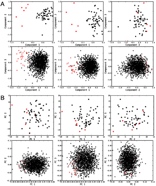
Figure 1: Low-dimensional representation of samples and variables from the synthetic data set, obtained by CUMBIA (panel A) and PCA (panel B). Sample representations are shown in the top row, and corresponding variable representations are shown below. Each subfigure shows the representation with respect to two of the three first components. Red markers represent the six samples and 25 variables which are simulated to be closely related. Black markers represent the other 54 samples and 1,475 variables in the data set (PC—principal component).

5.2 Microarray data set—human cell cultures.

Next, we consider a real microarray data set, from a study of gene expression profiles from 61 normal human cell cultures. The cell cultures are taken from five cell types in 23 different tissues or organs, in total 31 different tissue/cell type combinations. The data set was downloaded from the National Center for Biotechnology Informations (NCBI) Gene Expression Omnibus (GEO, http://www.ncbi. nlm.nih.gov/geo/, data set GDS1402). The original data set consists of 19,664 variables. We remove the variables containing missing values (2,741 variables) or negative expression values (another 517 variables), and the remaining values are $\log_{2}$-transformed.

To illustrate the ability of CUMBIA to detect small sample and variable clusters, we create a new data set from a subset of the variables in the microarray data set. We select two of the nontrivial sample subgroups, cardiac stromal cells ($N_{1}=3$) and umbilical artery endothelial cells ($N_{2}=6$). For each of these sample subgroups and for each variable, we perform a $t$-test contrasting the selected subgroup against all other samples. For each of the two subgroups, we include the 50 variables having the highest positive value of the $t$-statistic. We further extend the new data set with the 1,500 variables showing the least discriminative power (the lowest value of the $F$-statistic) in an $F$-test contrasting all 31 subgroups. Finally, all variables are mean centered and scaled to unit variance across the samples. The final data set now consists of $p=1\mbox{,}600$ variables and $N=61$ samples. This data set contains two relatively small sample groups, each of which is characterized by high values for a small subset of the variables. Furthermore, the vast majority ($93.75\%$) of the variables are not related to any of the predefined subgroups. Figure 2 shows the low-dimensional representations of the samples and variables obtained by CUMBIA (panel A) and PCA (panel B). The first two CUMBIA components successfully pick up the two small sample subgroups as well as the variables which are responsible for their close relation. These patterns do not encode enough variance to be seen in any of the three first principal components (panel B). In the projection onto the fourth and fifth principal components, the three cardiac stromal cell samples are visible as well as four of the six umbilical artery endothelial cells (data not shown). Clearly, by considering not only the variance of the extracted components as a measure of informativeness, CUMBIA highlights other features than PCA. Scree plots are available as the Supplementary Material. We used $d=10$ principal components for the whitening preceding the projection pursuit algorithm, which is able to detect the group of cardiac stromal cells, but the umbilical artery cells are considerably harder to extract (see the Supplementary Figures). The projection pursuit algorithm further finds one single umbilical artery cell occupying one component together with a group of underexpressed variables. By modifying the CUMBIA algorithm to search for both over- and underexpressed variables, we also find this pattern (see the Supplementary Material, Figure S2). For this data set, SAMBA returns 26 biclusters with significant overlaps. Eleven of these contain two of the cardiac stromal cells (but none of them contain all three). Eight biclusters contain at least two umbilical artery endothelial cell samples (one contains all six). Again, we note that the purpose of biclustering is not quite the same as the purpose of visualization which can also be seen in this example.

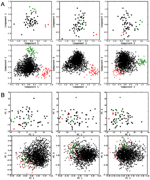
Figure 2: Low-dimensional representation of samples and variables from the human cell culture microarray data set, obtained by CUMBIA (panel A) and PCA (panel B). Red markers represent samples from the cardiac stromal cells ($N_{1}=3$), and the 50 variables with highest discriminative power for this sample group, respectively. Green markers similarly represent the umbilical artery endothelial cells ($N_{2}=6$) and the corresponding variables. Black markers represent samples from all other subgroups, and the 1,500 variables from the original data set which are least discriminating in an $F$-test contrasting all 31 tissue/cell type combinations in the data set.

5.3 MicroRNA data set—leukemia cell lines.

In the previous examples we have shown that for data sets where the main nonrandom variation is attributable to small groups of samples sharing extreme values for small groups of variables, CUMBIA can produce sample and variable visualizations that are more informative than those resulting from PCA and the applied projection pursuit algorithm. Now, we consider a data set containing measurements of 1,145 microRNAs in 20 human leukemia cell lines (unpublished data). The cell lines correspond to three different leukemia types; CML (chronic myeloid leukemia), AML (acute myeloid leukemia) and B-ALL (B-cell acute lymphoblastic leukemia). Figure 3 shows the visualizations obtained by CUMBIA and PCA. In this case, the feature distinguishing three of the CML samples (red markers) from the rest of the samples contains enough variance to be picked up by PCA. The discrimination of these samples is apparent also with CUMBIA, where furthermore the third component effectively discriminates the AML group (blue) from the B-ALL group (green). This effect is more readily visible than in the PCA visualization. The CML group is biologically heterogeneous which can also be seen in the visualizations. To facilitate the interpretation of the visualizations, we have colored all variables which are significantly higher expressed in one sample group than in the others. The heterogeneity of the CML group is reflected also here, in that some of the variables which are closely related to the three deviating CML samples are not significantly differentially expressed in the whole CML group. On the other hand, it is clear that the variables which have the most negative values on the third CUMBIA component are all highly expressed in the closely located AML samples (blue). Scree plots for CUMBIA and PCA are available in the Supplementary Material. We used $d=5$ principal components in the whitening for projection pursuit, and the resulting components are shown in the Supplementary Figures. In this case, the sample representations from projection pursuit results are not very different from those of CUMBIA, but the coupling between the salient sample groups and the corresponding discriminating variables is stronger with CUMBIA. In the absence of external annotations, this possibly enables formulating sharper and more correct hypotheses. Applying SAMBA to this data set returns 16 biclusters. Generally, from these biclusters it is difficult to extract information distinguishing the three leukemia subtypes.

Figure 3: Low-dimensional representation of samples and variables from the microRNA data set, obtained by CUMBIA (panel A) and PCA (panel B). Red markers represent samples from the CML subgroup, blue markers correspond to the AML group and green markers to the B-ALL group. Variables shown in one of these colors are significantly higher expressed in the corresponding sample group than in the other two (Student’s $t$-test, one-tailed $p<0.0005$, note that this information was not used to obtain the visualizations, but is merely displayed to facilitate the interpretation).

Taken together, the examples indicate that CUMBIA is a useful complement to existing visualization methods in different contexts. It can find features commonly detected by existing methods such as PCA and projection pursuit, but also features that are difficult to find with these methods.

6 Discussion and conclusions.

We have described CUMBIA: an unsupervised algorithm for exploratory analysis and simultaneous visualization of the samples and variables of a multivariate data set. The basis of the algorithm is classical multidimensional scaling (MDS), which is applied to a joint dissimilarity matrix and produces a common low-dimensional representation of samples and variables. The dissimilarity between a sample and a variable is based on the expression level of the variable in the sample; a higher expression level gives a lower dissimilarity. The dissimilarity between two samples (or two variables) is then defined by graph distances, influenced mainly by the variables (samples) with a high total expression level in the two samples (variables). By applying the method to a synthetic as well as real-world data sets, we have shown its ability to extract relevant sample and variable groups. Compared to PCA, which is commonly used for visualization of high-dimensional data, the proposed method is advantageous for extracting small related variable and sample subgroups. According to the proposed dissimilarity measure, two samples will be considered close if they share a high value of one or a small group of variables. This is in contrast to PCA, where the entire variable profiles are used to calculate the distance between a pair of samples. We believe that the proposed method may be a valuable complement to existing methods for exploratory analysis of multivariate data, to extract closely related sample clusters and immediately find the variables which are responsible for the discrimination. This group of variables can then be analyzed further and may constitute potential biomarkers for the corresponding sample group. As described in this paper, the proposed algorithm is mainly directed toward finding groups of samples sharing a high expression value of a, possibly small, group of variables, but can be adjusted to emphasize also jointly underexpressed variables.

By choosing different values of $K$ (the number of paths to average over in the calculation of the CUMBIA dissimilarities), it is possible to detect different structures. A small value of $K$ makes it possible to find very small sample and variable groups but makes the method sensitive to noisy data. With increasing $K$ the method becomes more robust, but it is also more difficult to detect the smallest groups. In an exploratory study, CUMBIA could be applied with different values of $K$ to find as many potentially relevant patterns as possible.

Putting the negative eigenvalues to zero in the classical MDS as we have done in this paper potentially discards interesting information, as discussed by Laub and Müller (2004). Interestingly, in the examples that we have given most eigenvalues are positive, but there is one large negative eigenvalue which corresponds to an eigenvector separating the sample objects from the variable objects. However, since we are mainly interested in the interaction between samples and variables, we focus on the largest positive eigenvalues of the inner product matrix and the corresponding eigenvectors.

The induced dissimilarities from CUMBIA may be potentially useful for clustering of samples and/or variables, for example, by hierarchical clustering [Sneath (1957); Hastie, Tibshirani and Friedman (2009)]. One would then expect small sample groups, characterized by few variables, to be clustered more closely than with hierarchical clustering based on, for example, Euclidean distance. The dissimilarities can potentially also be used for simultaneous feature and sample selection from the data set by backward feature elimination, in a manner similar, for example, to the “gene shaving” [Hastie et al. (2000)] and “recursive feature elimination” [Guyon et al. (2002)] procedures. This could be done in the following way. First, the joint CUMBIA dissimilarity matrix for the entire data set is calculated. Then, for each object (sample or variable), the mean value of the $K_{0}$ smallest dissimilarities between the object and all objects of the same type (i.e., samples or variables) are calculated for a suitable choice of $K_{0}$. A given fraction of the objects, consisting of those with the largest value of the mean dissimilarity score, can then be removed. This gives a new data matrix, with fewer samples and variables, to which the process may be applied. This algorithm provides a sequence of nested sample–variable biclusters. The optimal cluster size should be determined based on a suitably chosen optimality criterion. Furthermore, when a bicluster has been found, the included variables and samples may be removed from the data set and another, disjoint bicluster may be found from the resulting matrix.

Supplementary material [doi]10.1214/11-AOAS460SUPPA [url]http://lib.stat.cmu.edu/aoas/460/supplementA.pdf .pdf In the supplementary material we give a small schematic example showing the different steps of CUMBIA. Further, we show how to emphasize both over- and underexpressed variables in the visualization and how the choice of $K$ and $s$ affect the resulting visualization. We also provide scree plots obtained by CUMBIA and PCA for the three data sets studied in the paper. Supplementary figures—Projection pursuit results
[doi,text=10.1214/11-AOAS460SUPPB]10.1214/11-AOAS460SUPPB [url]http://lib.stat.cmu.edu/aoas/460/supplementB.pdf .pdf The supplementary figures show the result of the FastICA projection pursuit algorithm applied to the three data sets considered in the paper. Note that to facilitate the interpretation of the figures, the axes are ungraded and only the origin is marked.

References

- Alter, Brown and Botstein (2000) {barticle}[author] \bauthor\bsnmAlter, \bfnmO\binitsO., \bauthor\bsnmBrown, \bfnmP\binitsP. and \bauthor\bsnmBotstein, \bfnmD\binitsD. (\byear2000). \btitleSingular value decomposition for genome-wide expression data processing and modeling. \bjournalProc. Natl. Acad. Sci. USA \bvolume97 \bpages10101–10106. \endbibitem
- Belkin and Niyogi (2003) {barticle}[author] \bauthor\bsnmBelkin, \bfnmM\binitsM. and \bauthor\bsnmNiyogi, \bfnmP\binitsP. (\byear2003). \btitleLaplacian eigenmaps for dimensionality reduction and data representation. \bjournalNeural Comput. \bvolume15 \bpages1373–1396. \endbibitem
- Ben-Dor et al. (2003) {barticle}[author] \bauthor\bsnmBen-Dor, \bfnmA\binitsA., \bauthor\bsnmChor, \bfnmB\binitsB., \bauthor\bsnmKarp, \bfnmR\binitsR. and \bauthor\bsnmYakhini, \bfnmZ\binitsZ. (\byear2003). \btitleDiscovering local structure in gene expression data: The order-preserving submatrix problem. \bjournalJ. Comput. Biol. \bvolume10 \bpages373–384. \endbibitem
- Bergmann, Ihmels and Barkai (2003) {barticle}[author] \bauthor\bsnmBergmann, \bfnmS\binitsS., \bauthor\bsnmIhmels, \bfnmJ\binitsJ. and \bauthor\bsnmBarkai, \bfnmN\binitsN. (\byear2003). \btitleIterative signature algorithm for the analysis of large-scale gene expression data. \bjournalPhys. Rev. E \bvolume67 \bpages031902. \endbibitem
- Bisson and Hussain (2008) {binproceedings}[author] \bauthor\bsnmBisson, \bfnmG\binitsG. and \bauthor\bsnmHussain, \bfnmF\binitsF. (\byear2008). \btitleChi-Sim: A new similarity measure for the co-clustering task. In \bbooktitleProc. 2008 Seventh International Conference on Machine Learning and Applications \bpages211–217. \bpublisherIEEE Computer Society, \baddressLos Alamitos, CA. \endbibitem
- Cailliez (1983) {barticle}[author] \bauthor\bsnmCailliez, \bfnmF\binitsF. (\byear1983). \btitleThe analytical solution of the additive constant problem. \bjournalPsychometrika \bvolume48 \bpages305–308. \MR0721286 \endbibitem
- Chapman et al. (2001) {barticle}[author] \bauthor\bsnmChapman, \bfnmS\binitsS., \bauthor\bsnmSchenk, \bfnmP\binitsP., \bauthor\bsnmKazan, \bfnmK\binitsK. and \bauthor\bsnmManners, \bfnmJ\binitsJ. (\byear2001). \btitleUsing biplots to interpret gene expression patterns in plants. \bjournalBioinformatics \bvolume1 \bpages202–204. \endbibitem
- Cheng and Church (2000) {binproceedings}[author] \bauthor\bsnmCheng, \bfnmY\binitsY. and \bauthor\bsnmChurch, \bfnmG M\binitsG. M. (\byear2000). \btitleBiclustering of expression data. In \bbooktitleProc. ISMB’00 \bpages93–103. \bpublisherAAAI Press, \baddressMenlo Park, CA. \endbibitem
- Cox and Cox (2001) {bbook}[author] \bauthor\bsnmCox, \bfnmT F\binitsT. F. and \bauthor\bsnmCox, \bfnmM A A\binitsM. A. A. (\byear2001). \btitleMultidimensional Scaling, \bedition2nd ed. \bpublisherChapman & Hall, \baddressLondon. \endbibitem
- De Crespin de Billy, Dolédec and Chessel (2000) {barticle}[author] \bauthor\bparticleDe Crespin de \bsnmBilly, \bfnmV\binitsV., \bauthor\bsnmDolédec, \bfnmS\binitsS. and \bauthor\bsnmChessel, \bfnmD\binitsD. (\byear2000). \btitleBiplot presentation of diet composition data: An alternative or fish stomach contents analysis. \bjournalJ. Fish Biol. \bvolume56 \bpages961–973. \endbibitem
- Dhillon (2001) {binproceedings}[author] \bauthor\bsnmDhillon, \bfnmI S\binitsI. S. (\byear2001). \btitleCo-clustering documents and words using bipartite spectral graph partitioning. In \bbooktitleProc. KDD’01 \bpages269–274. \bpublisherACM, \baddressNew York. \endbibitem
- Eckart and Young (1936) {barticle}[author] \bauthor\bsnmEckart, \bfnmC\binitsC. and \bauthor\bsnmYoung, \bfnmG\binitsG. (\byear1936). \btitleThe approximation of one matrix by another of lower rank. \bjournalPsychometrika \bvolume1 \bpages211–218. \endbibitem
- Friedman and Tukey (1974) {barticle}[author] \bauthor\bsnmFriedman, \bfnmJ H\binitsJ. H. and \bauthor\bsnmTukey, \bfnmJ W\binitsJ. W. (\byear1974). \btitleA projection pursuit algorithm for exploratory data analysis. \bjournalIEEE Trans. Comput. \bvolumeC-23 \bpages881–890. \endbibitem
- Gabriel (1971) {barticle}[author] \bauthor\bsnmGabriel, \bfnmK R\binitsK. R. (\byear1971). \btitleThe biplot graphic display of matrices with application to principal component analysis. \bjournalBiometrika \bvolume58 \bpages453–467. \MR0312645 \endbibitem
- Getz, Levine and Domany (2000) {barticle}[author] \bauthor\bsnmGetz, \bfnmG\binitsG., \bauthor\bsnmLevine, \bfnmE\binitsE. and \bauthor\bsnmDomany, \bfnmE\binitsE. (\byear2000). \btitleCoupled two-way clustering analysis of gene microarray data. \bjournalProc. Natl. Acad. Sci. USA \bvolume97 \bpages12079–12084. \endbibitem
- Gower (1966) {barticle}[author] \bauthor\bsnmGower, \bfnmJ C\binitsJ. C. (\byear1966). \btitleSome distance properties of latent root and vector methods used in multivariate analysis. \bjournalBiometrika \bvolume53 \bpages325–338. \MR0214224 \endbibitem
- Gower and Hand (1996) {bbook}[author] \bauthor\bsnmGower, \bfnmJ C\binitsJ. C. and \bauthor\bsnmHand, \bfnmD J\binitsD. J. (\byear1996). \btitleBiplots, \bedition1st ed. \bpublisherChapman & Hall, \baddressLondon. \MR1382860 \endbibitem
- Gower and Harding (1988) {barticle}[author] \bauthor\bsnmGower, \bfnmJ C\binitsJ. C. and \bauthor\bsnmHarding, \bfnmS A\binitsS. A. (\byear1988). \btitleNonlinear biplots. \bjournalBiometrika \bvolume75 \bpages445–455. \MR0967583 \endbibitem
- Guyon et al. (2002) {barticle}[author] \bauthor\bsnmGuyon, \bfnmI\binitsI., \bauthor\bsnmWeston, \bfnmJ\binitsJ., \bauthor\bsnmBarnhill, \bfnmS\binitsS. and \bauthor\bsnmVapnik, \bfnmV\binitsV. (\byear2002). \btitleGene selection for cancer classification using support vector machines. \bjournalMach. Learn. \bvolume46 \bpages389–422. \endbibitem
- Hastie, Tibshirani and Friedman (2009) {bbook}[author] \bauthor\bsnmHastie, \bfnmT\binitsT., \bauthor\bsnmTibshirani, \bfnmR\binitsR. and \bauthor\bsnmFriedman, \bfnmJ\binitsJ. (\byear2009). \btitleThe Elements of Statistical Learning, \bedition2nd ed. \bpublisherSpringer, \baddressNew York. \MR2722294 \endbibitem
- Hastie et al. (2000) {barticle}[author] \bauthor\bsnmHastie, \bfnmT\binitsT., \bauthor\bsnmTibshirani, \bfnmR\binitsR., \bauthor\bsnmEisen, \bfnmM B\binitsM. B., \bauthor\bsnmAlizadeh, \bfnmA\binitsA., \bauthor\bsnmLevy, \bfnmR\binitsR., \bauthor\bsnmStaudt, \bfnmL\binitsL., \bauthor\bsnmChan, \bfnmW C\binitsW. C., \bauthor\bsnmBotstein, \bfnmD\binitsD. and \bauthor\bsnmBrown, \bfnmP\binitsP. (\byear2000). \btitle‘Gene shaving’ as a method for identifying distinct sets of genes with similar expression patterns. \bjournalGenome Biol. \bvolume1 \bpages1–21. \endbibitem
- Hotelling (1933a) {barticle}[author] \bauthor\bsnmHotelling, \bfnmH\binitsH. (\byear1933a). \btitleAnalysis of a complex of statistical variables into principal components. \bjournalJ. Educ. Psychol. \bvolume24 \bpages417–441. \endbibitem
- Hotelling (1933b) {barticle}[author] \bauthor\bsnmHotelling, \bfnmH\binitsH. (\byear1933b). \btitleAnalysis of a complex of statistical variables into principal components (continued from September issue). \bjournalJ. Educ. Psychol. \bvolume24 \bpages498–520. \endbibitem
- Huber (1985) {barticle}[author] \bauthor\bsnmHuber, \bfnmP\binitsP. (\byear1985). \btitleProjection pursuit. \bjournalAnn. Statist. \bvolume13 \bpages435–475. \MR0790553 \endbibitem
- Hyvärinen and Oja (2000) {barticle}[author] \bauthor\bsnmHyvärinen, \bfnmA\binitsA. and \bauthor\bsnmOja, \bfnmE\binitsE. (\byear2000). \btitleIndependent component analysis: Algorithms and applications. \bjournalNeural Netw. \bvolume13 \bpages411–430. \endbibitem
- Jolliffe (2002) {bbook}[author] \bauthor\bsnmJolliffe, \bfnmI T\binitsI. T. (\byear2002). \btitlePrincipal Component Analysis, \bedition2nd ed. \bpublisherSpringer, \baddressNew York. \MR2036084 \endbibitem
- Laub and Müller (2004) {barticle}[author] \bauthor\bsnmLaub, \bfnmJ\binitsJ. and \bauthor\bsnmMüller, \bfnmK-R\binitsK.-R. (\byear2004). \btitleFeature discovery in non-metric pairwise data. \bjournalJ. Mach. Learn. Res. \bvolume5 \bpages801–818. \MR2248000 \endbibitem
- Lee et al. (2010) {barticle}[author] \bauthor\bsnmLee, \bfnmM\binitsM., \bauthor\bsnmShen, \bfnmH\binitsH., \bauthor\bsnmHuang, \bfnmJ Z\binitsJ. Z. and \bauthor\bsnmMarron, \bfnmJ S\binitsJ. S. (\byear2010). \btitleBiclustering via sparse singular value decomposition. \bjournalBiometrics \bvolume66 \bpages1087–1095. \endbibitem
- Madeira and Oliveira (2004) {barticle}[author] \bauthor\bsnmMadeira, \bfnmS C\binitsS. C. and \bauthor\bsnmOliveira, \bfnmA L\binitsA. L. (\byear2004). \btitleBiclustering algorithms for biological data analysis: A survey. \bjournalIEEE/ACM Trans. Comput. Biol. Bioinform. \bvolume1 \bpages24–45. \endbibitem
- Mardia (1978) {barticle}[author] \bauthor\bsnmMardia, \bfnmK V\binitsK. V. (\byear1978). \btitleSome properties of classical multidimensional scaling. \bjournalComm. Statist. Theory Methods \bvolume7 \bpages1233–1241. \MR0514645 \endbibitem
- Park et al. (2008) {barticle}[author] \bauthor\bsnmPark, \bfnmM\binitsM., \bauthor\bsnmLee, \bfnmJ W\binitsJ. W., \bauthor\bsnmLee, \bfnmJ B\binitsJ. B. and \bauthor\bsnmSong, \bfnmS H\binitsS. H. (\byear2008). \btitleSeveral biplot methods applied to gene expression data. \bjournalJ. Statist. Plann. Inference \bvolume138 \bpages500–515. \MR2412601 \endbibitem
- Pearson (1901) {barticle}[author] \bauthor\bsnmPearson, \bfnmK\binitsK. (\byear1901). \btitleOn lines and planes of closest fit to systems of points in space. \bjournalPhil. Mag. (6) \bvolume2 \bpages559–572. \endbibitem
- Phillips and McNicol (1986) {barticle}[author] \bauthor\bsnmPhillips, \bfnmM S\binitsM. S. and \bauthor\bsnmMcNicol, \bfnmJ W\binitsJ. W. (\byear1986). \btitleThe use of biplots as an aid to interpreting interactions between potato clones and populations of potato cyst nematodes. \bjournalPlant Pathol. \bvolume35 \bpages185–195. \endbibitem
- Rege, Dong and Fotouhi (2008) {barticle}[author] \bauthor\bsnmRege, \bfnmM\binitsM., \bauthor\bsnmDong, \bfnmM\binitsM. and \bauthor\bsnmFotouhi, \bfnmF\binitsF. (\byear2008). \btitleBipartite isoperimetric graph partitioning for data co-clustering. \bjournalData Min. Knowl. Discov. \bvolume16 \bpages276–312. \MR2399022 \endbibitem
- Ross et al. (2003) {barticle}[author] \bauthor\bsnmRoss, \bfnmM E\binitsM. E., \bauthor\bsnmZhou, \bfnmX\binitsX., \bauthor\bsnmSong, \bfnmG\binitsG., \bauthor\bsnmShurtleff, \bfnmS A\binitsS. A., \bauthor\bsnmGirtman, \bfnmK\binitsK., \bauthor\bsnmWilliams, \bfnmW K\binitsW. K., \bauthor\bsnmLiu, \bfnmH-C\binitsH.-C., \bauthor\bsnmMahfouz, \bfnmR\binitsR., \bauthor\bsnmRaimondi, \bfnmS C\binitsS. C., \bauthor\bsnmLenny, \bfnmN\binitsN., \bauthor\bsnmPatel, \bfnmA\binitsA. and \bauthor\bsnmDowning, \bfnmJ R\binitsJ. R. (\byear2003). \btitleClassification of pediatric acute lymphoblastic leukemia by gene expression profiling. \bjournalBlood \bvolume102 \bpages2951–2959. \endbibitem
- Roweis and Saul (2000) {barticle}[author] \bauthor\bsnmRoweis, \bfnmS T\binitsS. T. and \bauthor\bsnmSaul, \bfnmL K\binitsL. K. (\byear2000). \btitleNonlinear dimensionality reduction by locally linear embedding. \bjournalScience \bvolume290 \bpages2323–2326. \endbibitem
- Schölkopf, Smola and Müller (1998) {barticle}[author] \bauthor\bsnmSchölkopf, \bfnmB\binitsB., \bauthor\bsnmSmola, \bfnmA J\binitsA. J. and \bauthor\bsnmMüller, \bfnmK-R\binitsK.-R. (\byear1998). \btitleNonlinear component analysis as a kernel eigenvalue problem. \bjournalNeural Comput. \bvolume10 \bpages1299–1319. \endbibitem
- Shamir et al. (2005) {barticle}[author] \bauthor\bsnmShamir, \bfnmR\binitsR., \bauthor\bsnmMaron-Katz, \bfnmA\binitsA., \bauthor\bsnmTanay, \bfnmA\binitsA., \bauthor\bsnmLinhart, \bfnmC\binitsC., \bauthor\bsnmSteinfeld, \bfnmI\binitsI., \bauthor\bsnmSharan, \bfnmR\binitsR., \bauthor\bsnmShiloh, \bfnmY\binitsY. and \bauthor\bsnmElkon, \bfnmR\binitsR. (\byear2005). \btitleEXPANDER—An integrative program suite for microarray data analysis. \bjournalBMC Bioinformatics \bvolume6 \bpages232. \endbibitem
- Sneath (1957) {barticle}[author] \bauthor\bsnmSneath, \bfnmP H A\binitsP. H. A. (\byear1957). \btitleThe application of computers to taxonomy. \bjournalJ. Gen. Microbiol. \bvolume17 \bpages201–226. \endbibitem
- Soneson and Fontes (2010) {bmisc}[author] \bauthor\bsnmSoneson, \bfnmC\binitsC. and \bauthor\bsnmFontes, \bfnmM\binitsM. (\byear2010). \bhowpublishedSupplement to “A method for visual identification of small sample subgroups and potential biomarkers.” DOI:10.1214/11-AOAS460SUPPA, DOI:10.1214/11-AOAS460SUPPB. \endbibitem
- Tanay, Sharan and Shamir (2002) {barticle}[author] \bauthor\bsnmTanay, \bfnmA\binitsA., \bauthor\bsnmSharan, \bfnmR\binitsR. and \bauthor\bsnmShamir, \bfnmR\binitsR. (\byear2002). \btitleDiscovering statistically significant biclusters in gene expression data. \bjournalBioinformatics \bvolume18 \bpagesS136–S144. \endbibitem
- Tenenbaum, de Silva and Langford (2000) {barticle}[author] \bauthor\bsnmTenenbaum, \bfnmJ B\binitsJ. B., \bauthor\bparticlede \bsnmSilva, \bfnmV\binitsV. and \bauthor\bsnmLangford, \bfnmJ C\binitsJ. C. (\byear2000). \btitleA global geometric framework for nonlinear dimensionality reduction. \bjournalScience \bvolume290 \bpages2319–2322. \endbibitem
- Torgerson (1952) {barticle}[author] \bauthor\bsnmTorgerson, \bfnmW S\binitsW. S. (\byear1952). \btitleMultidimensional scaling: I. Theory and method. \bjournalPsychometrika \bvolume17 \bpages401–419. \MR0054219 \endbibitem
- Wang et al. (2002) {binproceedings}[author] \bauthor\bsnmWang, \bfnmH\binitsH., \bauthor\bsnmWang, \bfnmW\binitsW., \bauthor\bsnmYang, \bfnmJ\binitsJ. and \bauthor\bsnmYu, \bfnmP S\binitsP. S. (\byear2002). \btitleClustering by pattern similarity in large data sets. In \bbooktitleProc. 2002 ACM SIGMOD \bpages394–405. \bpublisherACM, \baddressNew York. \endbibitem
- Wouters et al. (2003) {barticle}[author] \bauthor\bsnmWouters, \bfnmL\binitsL., \bauthor\bsnmGöhlmann, \bfnmH\binitsH., \bauthor\bsnmBijnens, \bfnmL\binitsL., \bauthor\bsnmKass, \bfnmS U\binitsS. U., \bauthor\bsnmMolenberghs, \bfnmG\binitsG. and \bauthor\bsnmLewi, \bfnmP J\binitsP. J. (\byear2003). \btitleGraphical exploration of gene expression data: A comparative study of three multivariate methods. \bjournalBiometrics \bvolume59 \bpages1131–1139. \MR2025698 \endbibitem