Efficient methods for sampling spike trains in networks of coupled neurons

Abstract

Monte Carlo approaches have recently been proposed to quantify connectivity in neuronal networks. The key problem is to sample from the conditional distribution of a single neuronal spike train, given the activity of the other neurons in the network. Dependencies between neurons are usually relatively weak; however, temporal dependencies within the spike train of a single neuron are typically strong. In this paper we develop several specialized Metropolis–Hastings samplers which take advantage of this dependency structure. These samplers are based on two ideas: (1) an adaptation of fast forward–backward algorithms from the theory of hidden Markov models to take advantage of the local dependencies inherent in spike trains, and (2) a first-order expansion of the conditional likelihood which allows for efficient exact sampling in the limit of weak coupling between neurons. We also demonstrate that these samplers can effectively incorporate side information, in particular, noisy fluorescence observations in the context of calcium-sensitive imaging experiments. We quantify the efficiency of these samplers in a variety of simulated experiments in which the network parameters are closely matched to data measured in real cortical networks, and also demonstrate the sampler applied to real calcium imaging data.

TITLSupported by a McKnight Scholar and NSF CAREER award, as well as Grant IIS-0904353 from the NSF.

and

1 Introduction

One of the central goals of neuroscience is to understand how the structure of neural circuits underlies the processing of information in the brain, and in recent years a considerable effort has been focused on measuring neural connectivity empirically [Shepherd, Pologruto and Svoboda (2003); Bureau, Shepherd and Svoboda (2004); Briggman and Denk (2006); Hagmann et al. (2007); Sato et al. (2007); Smith (2007); Hagmann et al. (2008); Luo, Callaway and Svoboda (2008); Bohland et al. (2009); Helmstaedter, Briggman and Denk (2009)]. “Functional” approaches to this neural connectivity problem rely on statistical analysis of neural activity observed with experimental techniques such as multielectrode extracellular recording [Hatsopoulos et al. (1998); Harris et al. (2003); Stein et al. (2004); Paninski (2004); Truccolo et al. (2005); Santhanam et al. (2006); Luczak et al. (2007); Pillow et al. (2008)] or calcium imaging [Tsien (1989); Cossart, Aronov and Yuste (2003); Yuste et al. (2006); Ohki et al. (2005)]. Although functional approaches [Brillinger (1988); Nykamp (2003); Nykamp (2005a); Okatan, Wilson and Brown (2005); Srinivasan et al. (2006); Rigat, de Gunst and van Pelt (2006); Nykamp (2007); Yu et al. (2006); Kulkarni and Paninski (2007)] have not yet been demonstrated to directly yield the true physical structure of a neural circuit, the estimates obtained via this type of analysis play an increasingly important role in attempts to understand information processing in neural circuits [Bureau, Shepherd and Svoboda (2004); Sato et al. (2007); Pillow et al. (2008); Mishchenko, Vogelstein and Paninski (2011)].

Perhaps the biggest challenge for inferring neural connectivity from functional data—and indeed in network analysis more generally—is the presence of hidden nodes which are not observed directly [Nykamp (2005b, 2007); Kulkarni and Paninski (2007); Vidne et al. (2009); Pillow and Latham (2007); Vakorin, Krakovska and McIntosh (2009)]. Despite swift progress in simultaneously recording activity in massive populations of neurons, it is still beyond the reach of current technology to monitor a complete set of neurons that provide the presynaptic inputs even for a single neuron [though see, e.g., Petreanu et al. (2009) for some recent progress in this direction]. Since estimation of functional connectivity relies on the analysis of the inputs to target neurons in relation to their observed spiking activity, the inability to monitor all inputs can result in persistent errors in the connectivity estimation due to model misspecification. Developing a principled and robust approach for incorporating such unobserved neurons, whose spike trains are unknown and constitute hidden or latent variables, is an area of active research in connectivity analysis [Nykamp (2007); Pillow and Latham (2007); Vidne et al. (2009); Vakorin, Krakovska and McIntosh (2009)].

Incorporating these latent variables into connectivity estimation is a challenging task. The standard approach for estimating the connectivity requires us to compute the likelihood of the observed neural activity given an estimate of the underlying connectivity. Computing this likelihood, however, requires us to integrate out the probability distribution over the activity of all hidden neurons. This latent activity variable will typically have very high dimensionality, making any direct integration methods infeasible.

Thus, it is natural to turn to Markov chain Monte Carlo (MCMC) approaches here [Rigat, de Gunst and van Pelt (2006)]. The best design of such an MCMC sampler is not at all obvious in this setting, since it may be necessary to develop sophisticated proposal densities to capture the dependence of the hidden spike trains on the observed spiking data in order to guarantee a reasonable proposal acceptance rate [Pillow and Latham (2007)]. For example, the simplest Gibbs sampling approaches may not perform well given the strong dependencies between adjacent spiking timebins that are inherent to neural activity.

In this paper we develop Metropolis–Hastings (MH) algorithms for efficiently sampling from the probability distribution over the activity of hidden neurons. We derive a proposal density that is asymptotically correct in the limit of weak interneuronal couplings, and demonstrate the utility of this proposal density on simulated networks of neurons with neurophysiologically feasible parameters [Sayer, Friedlander and Redman (1990); Abeles (1991); Braitenberg and Schuz (1998); Gómez-Urquijo et al. (2000); Song et al. (2005); Lefort, Tomm and Sarria (2009)]. We also consider a hybrid MH strategy based on fast hidden Markov model (HMM) sampling approaches that can be exploited to extend the range of applicability of the basic algorithm to more strongly coupled networks of neurons. In each case, the resulting MCMC chain mixes quickly and each step of the chain may be computed quickly.

Of special interest is the problem of sampling from the probability distribution over unknown spike trains when a neuron is indirectly observed using calcium imaging (instead of electrical recordings) [Tsien (1989); Yuste et al. (2006); Cossart, Aronov and Yuste (2003); Ohki et al. (2005); Vogelstein et al. (2009)]. This problem can be naturally related to the sampling problem described above. We develop an approach to incorporate calcium fluorescence imaging observations directly into our proposal density. This allows us to efficiently sample from the probability distribution over the activity of multiple hidden neurons given calcium fluorescence observations, improving on the methods introduced in Mishchenko, Vogelstein and Paninski (2011).

2 Methods

2.1 Model definition

We model the activity of individual neurons with a discrete-time generalized linear model (GLM) [Brillinger (1988); Chornoboy, Schramm and Karr (1988); Brillinger (1992); Plesser and Gerstner (2000); Paninski et al. (2004); Paninski (2004); Rigat, de Gunst and van Pelt (2006); Truccolo et al. (2005); Nykamp (2007); Kulkarni and Paninski (2007); Pillow et al. (2008); Vidne et al. (2009); Stevenson et al. (2009)]:

$$n_{i}(t) \sim \operatorname{Bernoulli}[f(J_{i}(t))\Delta],$$

$$J_{i}(t) = b_{i}(t)+\sum_{j=1}^{N}\sum_{t^{\prime}<t}w_{ij}(t-t^{\prime})n_{j}(t^{\prime}),$$

where the spike indicator function for neuron $i$, $n_{i}(t)\in\{0,1\}$, is defined on time bins $t$ of size $\Delta$. Connectivity between neurons is described via the “connectivity matrix,” $w_{ij}(t)$; the self-terms $w_{ii}(t-t^{\prime})$ describe refractory effects (there is a minimal “refractory” interspike interval of a millisecond or two in most neurons, e.g.), and $w_{ij}(t-t^{\prime})$ represents the statistical effect of a spike in neuron $j$ at time $t^{\prime}$ upon the spiking rate of neuron $i$ at time $t$. $N$ is the number of neurons in the neural population, including hidden and observed neurons, and $b_{i}(t)$ denotes a baseline driving term (which might depend on some observed covariates such as a sensory stimulus). We assume that the maximal firing frequency $\Delta^{-1}$ is much larger than the typical spiking rate, $\Delta^{-1}\gg E[n_{i}(t)]$, in which case the Bernoulli spiking model in (2.1) is closely related to models in which $n_{i}(t)$ is drawn from a Poisson distribution at every time step (see the references above for a number of examples).

In the presence of fluorescence observations from a calcium-sensitive indicator dye (the calcium imaging setting), the model (2.1) is supplemented by two variables per neuron $i$: the intracellular calcium concentration $C_{i}(t)$ (which is not observed directly) and the fluorescence observations $F_{i}(t)$. We model these terms according to a hidden Markov model governed by a simple driven autoregressive process [Vogelstein et al. (2009); Mishchenko, Vogelstein and Paninski (2011)],

$$C_{i}(t) = C_{i}(t-\Delta)-\frac{\Delta}{\tau^{c}_{i}}\bigl{(}C_{i}(t-\Delta)-C_{i}^{b}\bigr{)}+A_{i}n_{i}(t),$$

$$F_{i}(t) \sim \mathcal{N}[S(C_{i}(t)),V(C_{i}(t))].$$

Thus, under nonspiking conditions, $C_{i}(t)$ is set to the baseline level of $C_{i}^{b}$. Whenever the neuron fires a spike, $n_{i}(t)=1$, the calcium variable $C_{i}(t)$ jumps by a fixed amount $A_{i}$, and subsequently decays with time constant $\tau^{c}_{i}$; $\tau^{c}_{i}$ is on the order of hundreds of milliseconds in the cases of most interest here. The fluorescence signal $F_{i}(t)$ corresponds to the count of photons collected at the detector per neuron per imaging frame. This photon count may be modeled with approximately Gaussian statistics (Poisson photon count models are also tractable in this context [Vogelstein et al. (2009)], though we will not pursue this detail here), with the mean given by a saturating Hill-type function $S(C)=C/(C+K_{d})$ Yasuda et al. (2004) and the variance $V(C)$ scaling with the mean. See Vogelstein et al. (2009) for full details and further discussion. Note that observations of calcium-indicator fluorescence are typically performed at a low “frame-rate,” $\mathit{FR}$, measured in frames per second. Thus, we will restrict our attention to the case $\mathit{FR}<\Delta^{-1}$, that is, $F_{i}(t)$ observations are available only every few timesteps $\Delta$. In addition, it will be useful to define an effective SNR, following Mishchenko, Vogelstein and Paninski (2011), as

$$e\mathit{SNR}=\frac{E[F_{i}(t)-F_{i}(t-\Delta)|n_{i}(t)=1]}{E[(F_{i}(t)-F_{i}(t-\Delta))^{2}/2|n_{i}(t)=0]^{1/2}},$$ (3)

that is, the size of a spike-driven fluorescence jump divided by a rough measure of the standard deviation of the baseline fluorescence.

In Mishchenko, Vogelstein and Paninski (2011) we introduced an expectation-maximization approach for estimating the model parameters given calcium fluorescence data; Pillow and Latham (2007) discuss a related approach for fitting the model given spiking data recorded from extracellular electrodes. The maximization step in this context is often quite tractable, involving a separable convex optimization problem [Smith and Brown (2003); Paninski (2004); Kulkarni and Paninski (2007); Escola et al. (2011)]. The expectation step is much more difficult; analytical approaches are often infeasible. Monte Carlo solutions to this problem require us to obtain samples from the probability distribution over the activity of all hidden neurons. This problem is the focus of the present paper. In the context of the expectation maximization framework, we assume therefore that an estimate of the model parameters $\theta$ is available, and the problem is to obtain a sample from $P(\mathbf{n}_{\mathit{hidden}}|\mathbf{n}_{\mathit{observed}};\bolds{\theta})$ (in the case that the spike trains of a subset of neurons is observed directly), or $P(\mathbf{n}_{\mathit{hidden}}|\mathbf{F}_{\mathit{observed}};\bolds{\theta})$ (in the case that spike trains are observed indirectly via calcium fluorescence measurements). Here and throughout we use bold notation for vectors, that is, $\mathbf{n}(t)=\{n_{i}(t),i=1,\ldots,N\}$ and $\mathbf{n}=\{n_{i}(t),i=1,\ldots,N;t\in[0,T]\}$; $\theta$ denotes the set of all parameters in the model, including $\mathbf{b},\mathbf{w},\bolds{\tau}^{c}$, and $\mathbf{A}$. In cases where no confusion is possible below we will suppress the dependence on $\theta$.

2.2 A block-wise Gibbs approach for sampling from the distribution over activity of hidden neurons

In Mishchenko, Vogelstein and Paninski (2011), we noted that in order to sample from the desired joint distribution over the activity of all hidden neurons, $P(\mathbf{n}_{\mathit{hidden}}|\cdot)$, it is sufficient to be able to efficiently sample sequentially from the conditional distribution over one hidden neuron given all of the other hidden neurons, $P(\mathbf{n}_{i}|\mathbf{n}_{\setminus i};\cdot)$: if this is possible, then a sample from the full joint distribution, $P(\mathbf{n}_{\mathit{hidden}}|\cdot)$, can be obtained using a block-wise Gibbs algorithm. This blockwise Gibbs approach makes sense in this context because the connectivity weights $w_{ij},i\neq j$, are relatively weak in many neural contexts; for example, synaptic strengths between cortical neurons are typically fairly small (see the discussion in Section 2.7 below). However, dependencies between the spike indicator variables $\{n_{i}(s),n_{i}(t)\}$ within a single neuron may be quite large if the time gap $|s-t|$ is small, since the self-terms $w_{ii}$ are typically strong over small timescales; for example, as mentioned above, after every spike a neuron will enter a refractory state during which it is unable to spike again for some time period. See Toyoizumi, Rahnama Rad and Paninski (2009) for further discussion.

Thus, we will focus below exclusively on the single-neuron conditional sampling problem, $\mathbf{n}_{i}\sim P(\mathbf{n}_{i}|\mathbf{n}_{\setminus i};\cdot)$. In the next couple sections we will discuss methods for sampling from $P(\mathbf{n}_{i}|\mathbf{n}_{\setminus i})$; in Section 2.6 we will discuss adaptations of these methods for incorporating calcium fluorescence observations in $P(\mathbf{n}_{i}|\mathbf{n}_{\setminus i},\mathbf{F}_{i})$.

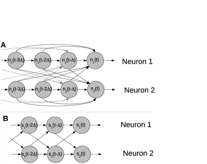
Figure 1: Graphical model describing (A) the $K$-order Markov model for neural dynamics in terms of the instantaneous spikes, $n_{i}(t)$, and (B) a simpler Markov model in terms of the grouped states $s_{i}(t)=\{n_{i}(t^{\prime}),t-K\Delta<t^{\prime}\leq t\}$.

2.3 Exact sampling via the hidden Markov model forward–backward procedure

In some special cases we can solve the single-neuron conditional sampling problem quite explicitly. Specifically, if the support of each of the coupling terms $w_{ij}(t)$ is contained in the interval $[0,K\Delta]$ for some sufficiently small number of time steps $K$, then we can employ standard hidden Markov model methods to sample from the desired conditional distribution exactly. The key is to note that in this case equation (2.1) defines a $K$th-order Markov process; thus, it is convenient to apply the standard substitution $s_{i}(t)=\{n_{i}(t^{\prime}),t-K\Delta<t^{\prime}\leq t\}$. Here $s_{i}(t)$ denotes the “state” of neuron $i$, which is completely characterized by the binary $K$-string [e.g., $s_{i}(t)=\mbox{``}010011100\ldots\mbox{''}$] describing its spiking over the $K$ most recent time bins. Clearly, the size of the state-space is $2^{K}$. See Figure 1 for an illustration.

To exploit this Markov structure, note that we may write the conditional distributions $P[s_{i}(t)|s_{i}(t-\Delta),\mathbf{s}_{\setminus i}(t-\Delta)]$ and $P[\mathbf{s}_{\setminus i}(t+\Delta)|\mathbf{s}_{\setminus i}(t),s_{i}(t)]$ explicitly using model (2.1), and, in fact, it is easy to see that the system

$$s_{i}(t) \sim P[s_{i}(t)|s_{i}(t-\Delta),\mathbf{s}_{\setminus i}(t-\Delta)],$$

$$\mathbf{s}_{\setminus i}(t+\Delta) \sim P[\mathbf{s}_{\setminus i}(t+\Delta)|\mathbf{s}_{\setminus i}(t),s_{i}(t)]$$

forms an autoregressive hidden Markov model [Rabiner (1989)], with $\mathbf{s}_{\setminus i}(t+\Delta)$ playing the role of the observation at time $t$ (Figure 1). Thus, if $K$ is not too large, standard finite hidden Markov model (HMM) techniques can be applied to obtain the desired spike train samples. Specifically, we can use the standard filter forward-sample backward algorithm [Rabiner (1989); De Gunst, Künsch and Schouten (2001)] to obtain samples from $P(\mathbf{s}_{i}|\mathbf{s}_{\setminus i})$, from which we can easily transform back to obtain the desired sample $\mathbf{n}_{i}$. This requires $O(T2^{K})$ computation time and $O(2^{K})$ memory, since the transition matrix $P[s_{i}(t)|s_{i}(t-\Delta),\mathbf{s}_{\setminus i}(t-\Delta)]$ is sparse [due to the redundant definition of the state variable $s_{i}(t)$], so the matrix–vector multiplication required in the transition step scales linearly with the number of states, instead of quadratically, as would be seen in the general case. Note, for clarity, that in the above discussion we are assuming that the coupling terms $w_{ij}(t)$ are known (or have been estimated in a separate step), and therefore $K$ is also known, directly from the maximal support of the couplings $w_{ij}(t)$; thus, we do not apply any model selection or estimation techniques for choosing $K$ here.

2.4 Efficient sampling in the weak-coupling limit

Clearly, the HMM strategy described above will become ineffective if $K$ becomes larger than about $10$ or so, due to the exponential growth of the Markov state-space. Therefore, it is natural to seek more general alternate methods. Recall that the interneuronal coupling terms $w_{ij},i\neq j$, are small. Thus, it seems promising to examine the conditional spike train probability in the limit of weak coupling ($w_{ij}\to 0$), in the hope that a good sampling method might suggest itself.

The log-likelihood of the hidden spike train $\mathbf{n}_{i}$ can be written as

$$\qquad\log P(\mathbf{n}_{i}|\mathbf{n}_{\setminus i}) = \log P(\mathbf{n}_{i},\mathbf{n}_{\setminus i})+\mbox{const.}$$

$$= \sum_{i}\sum_{t}n_{i}(t)\log f[J_{i}(t)]-f[J_{i}(t)]\Delta-n_{i}(t)!+\mbox{const.};$$

for notational simplicity, we have used a Poisson model for $n_{i}(t)$ given the past spike trains, but it turns out that we can use any exponential family with linear sufficient statistics in the following computations; see the Appendix for details. Now, if we make the abbreviation

$$J^{-}_{i}(t)=\sum_{s<t}\sum_{j}w_{ij}(t-s)n_{j}(s),$$ (6)

we can easily expand to first order in $w_{ij}$:

$$\log P(\mathbf{n}_{i},\mathbf{n}_{\setminus i})$$

$$\qquad=\sum_{t}n_{i}(t)\log f[J_{i}(t)]-f[J_{i}(t)]\Delta-n_{i}(t)!$$

$$\qquad\quad{}+\sum_{j\neq i}\sum_{t}n_{j}(t)\log f[b_{j}(t)+J^{-}_{j}(t)]-f[b_{j}(t)+J^{-}_{j}(t)]\Delta+\mbox{const.}$$

$$\qquad=\sum_{t}n_{i}(t)\log f[J_{i}(t)]-f[J_{i}(t)]\Delta-n_{i}(t)!$$

$$\qquad\quad{}+\sum_{j\neq i}\sum_{t}n_{j}(t)\log f[b_{j}(t)]-f[b_{j}(t)]\Delta$$

$$\qquad\quad\hphantom{{}+\sum_{j\neq i}\sum_{t}}{}+\biggl{(}n_{j}(t)\frac{f^{\prime}[b_{j}(t)]}{f[b_{j}(t)]}-f^{\prime}[b_{j}(t)]\Delta\biggr{)}J^{-}_{j}(t)+o(w)+\mbox{const.}$$

$$\qquad=\sum_{t}n_{i}(t)\log f[J_{i}(t)]-f[J_{i}(t)]\Delta-n_{i}(t)!$$

$$\qquad\quad{}+\sum_{j\neq i}\sum_{t}\biggl{(}n_{j}(t)\frac{f^{\prime}[b_{j}(t)]}{f[b_{j}(t)]}-f^{\prime}[b_{j}(t)]\Delta\biggr{)}\sum_{s<t}\sum_{k}w_{jk}(t-s)n_{k}(s)$$

$$\qquad\quad{}+o(w)+\mbox{const.}$$

$$\qquad=\sum_{t}n_{i}(t)\log f[J_{i}(t)]-f[J_{i}(t)]\Delta-n_{i}(t)!$$ (7)

$$\qquad\quad{}+\sum_{j\neq i}\sum_{t}\sum_{s>t}\biggl{(}n_{j}(s)\frac{f^{\prime}[b_{j}(s)]}{f[b_{j}(s)]}-f^{\prime}[b_{j}(s)]\Delta\biggr{)}w_{ji}(s-t)n_{i}(t)$$

$$\qquad\quad{}+o(w)+\mbox{const.}$$

$$\qquad=\sum_{t}n_{i}(t)\biggl{\{}\log f[J_{i}(t)]+\sum_{j\neq i}\sum_{s>t}\frac{f^{\prime}[b_{j}(s)]}{f[b_{j}(s)]}w_{ji}(s-t)[n_{j}(s)-f[b_{j}(s)]\Delta]\biggr{\}}$$

$$\qquad\quad\hphantom{\sum_{t}}{}-n_{i}(t)!+o(w)+\mbox{const.},$$

where we have used the definition of $J^{-}_{j}(t)$ in the third equality, rearranged sums (and changed variables) over $t$ and $s$ in the fourth equality, regathered terms in the final equality, and retained only terms involving a factor of $n_{i}(t)$ throughout.

Thus, if we note the resemblance between equation (2.4) and the Poisson log-probability, we see that one attractive approach is to sample from a spike train proposal $n_{i}(t)$ with log-rate equal to the term within brackets,

$$\log f[J_{i}(t)]+\sum_{j\neq i}\sum_{s>t}\frac{f^{\prime}[b_{j}(s)]}{f[b_{j}(s)]}w_{ji}(s-t)\bigl{[}n_{j}(s)-f[b_{j}(s)]\Delta\bigr{]};$$ (8)

since we are conditioning on $\{n_{j}(t)\}$ (i.e., these terms are assumed fixed), and there are no $n_{i}(s)$ terms affecting the proposed rate of $n_{i}(t)$ for $s>t$, it is straightforward to sample $n_{i}(t)$ recursively forward according to this rate, and then use Metropolis–Hastings to compute the required acceptance probability and obtain a sample from the desired distribution.

We note that this approach is conceptually quite similar to that of Pillow and Latham (2007), who proposed sampling recursively from a process of the form

$$n_{i}(t) \sim \mbox{Poisson}[f[J^{\mathit{PL}}_{i}(t)]\Delta],$$

$$J^{\mathit{PL}}_{i}(t) = b^{\mathit{PL}}_{i}+\sum_{j}\sum_{s<t}w^{\mathit{PL}}_{ij}(t-s)n_{j}(s)+\sum_{j\neq i}\sum_{s>t}w^{\mathit{PL}}_{ij}(t-s)n_{i}(s).$$

Pillow and Latham (2007) discussed a somewhat computationally-intensive procedure in which the parameters $b_{i}^{\mathit{PL}}$ and $w_{ij}^{\mathit{PL}}$ are reoptimized iteratively via a maximum pseudolikelihood procedure. If we reverse the logic we used to obtain equation (2.4), it is clear that our approach simply uses an “effective input”

$$\tilde{J}_{i}(t) = b_{i}(t)+J^{-}_{i}(t)$$

$${}+\sum_{j\neq i}\sum_{s>t}\frac{f[b_{i}(t)]}{f^{\prime}[b_{i}(t)]}\frac{f^{\prime}[b_{j}(s)]}{f[b_{j}(s)]}w_{ji}(s-t)\bigl{[}n_{j}(s)-f[b_{j}(s)]\Delta\bigr{]}$$

in place of $J_{i}^{\mathit{PL}}(t)$ above. Further, in the special case of an exponential nonlinearity, $f(J)=\exp(J)$, all pre-factors in equation (2.4) cancel out, leading to an expression that resembles equation (2.4) quite closely:

$$\tilde{J}_{i}(t) = b_{i}(t)+\sum_{j}\sum_{s<t}w_{ij}(t-s)n_{j}(s)$$

$${}+\sum_{j\neq i}\sum_{s>t}w_{ji}(s-t)\bigl{[}n_{j}(s)-f[b_{j}(s)]\Delta\bigr{]}.$$

Thus, in the weak-coupling limit $w\to 0$, and ignoring self-interactionterms $w_{ii}$, we see that the optimal “back-inputs” $w^{\mathit{PL}}_{ij}(t-s),s>t$, from Pillow and Latham (2007) may be analytically identified as the time- and index-reversed original forward couplings, $w_{ji}(-t)$.

2.5 Hybrid HMM-Metropolis–Hastings approaches

So far we have developed two methods for sampling from $P(\mathbf{n}_{i}|\mathbf{n}_{\setminus i})$: the HMM method (Section 2.3) is exact but becomes inefficient when $K$ is large, while the weak-coupling method (Section 2.4) becomes inefficient when the coupling terms $w$ become large. What is needed is a hybrid approach that combines the strengths of these two methods. The key is that the cross-coupling terms $w_{ij}$ are typically fairly weak (as emphasized above), and the self-couplingterms $w_{ii}(t)$ are large only for a small number of time delays $t$.

To take advantage of this special structure, we begin by constructing a truncated HMM that retains all coupling terms $w_{ij}(t)$ for $t$ up to some maximal delay $t_{\max}$, where $t_{\max}$ is chosen to keep the size of the state-space acceptably small but large enough so that the coupling terms are captured to an acceptable degree. Then we include the discarded coupling terms (i.e., terms at lags longer than $t_{\max}$) via the first-order approximation. More concretely, denote the conditional probability of $\{n_{i}(t)\}$ under the truncated HMM as

$$\prod_{t}P_{hmm}\bigl{(}s_{i}(t)|s_{i}(t-\Delta);\mathbf{n}_{\setminus i}\bigr{)}$$ (12)

[recall the correspondence between the $K$-string state variable $s_{i}(t)$ and the binary spiking variable $n_{i}(t)$]. Note that this forms an inhomogeneous Markov chain in the grouped state variables $s_{i}(t)$, and an inhomogeneous ($t_{\max}/\Delta$)-Markov chain in $n_{i}(t)$, as discussed in Section 2.3. Now we want to incorporate the discarded coupling terms up to the first order: we simply form the product

$$\prod_{t}P_{hmm}\bigl{(}s_{i}(t)|s_{i}(t-\Delta);\mathbf{s}_{\setminus i}\bigr{)}$$

$$\qquad{}\times\exp\biggl{(}n_{i}(t)\sum_{j\neq i}\sum_{t^{\prime}>t_{\max}}w_{ji}(t^{\prime}-t)\frac{f^{\prime}(b_{j}(t^{\prime}))}{f(b_{j}(t^{\prime}))}[n_{j}(t^{\prime})-f(b_{j}(t^{\prime}))\Delta]\biggr{)}.$$

We use this simple product form here in an analogy to the HMM case, in which we condition on observations by simply forming the (normalized) product of the prior distribution on state variables and the likelihood of the observations given the state variables; in this case, the first term plays the role of the prior over the state variables $s_{i}(t)$ and the second term corresponds to the pseudo-observations represented by the weak coupling terms incorporating the observed firing of the other neurons $n_{j}$. Although, to be clear, this joint probability does not correspond rigorously to any small-parameter expansion of $P(\mathbf{n}_{i}|\mathbf{n}_{\setminus i})$, we might expect that this hybrid may outperform alternative strategies such as using only the truncated HMM, given by equation (12), or only the weak-coupling correction, given by equation (2.5), as we will see in the Results section below (see especially Figure 6). Since this product form for the joint probability is structurally equivalent to the conditional probability of an HMM in the state variables $s_{i}(t)$—more precisely, the graphical model [Jordan (1999)] corresponding to the above expression is a chain in terms of $s_{i}(t)$—we can employ the forward–backward procedure to sample from this proposal, and then compute the Metropolis–Hastings acceptance probability to obtain samples from the desired conditional $P(\mathbf{n}_{i}|\mathbf{n}_{\setminus i})$.

Note that the MH acceptance probability will decrease as a function of the dimensionality $T$ of the desired spike train and of the size of the discarded weights $w_{ij}(t),t>t_{\max}$, since for large $w$ the proposal density discussed above will approximate the target density less accurately. In general, it is necessary to employ a blockwise approach: that is, we update the spike train $\{n_{i}(t)\}$ in blocks whose length is chosen to be small enough that the MH acceptance probability is sufficiently high, but large enough so that the total correlations between blocks are small and the overall chain mixes quickly. We will examine these trade-offs in more quantitative detail in the Results section below.

2.6 Efficient sampling given calcium fluorescence imaging observations

In this section we turn our attention to the problem of sampling from the fluorescent-conditional distribution $\mathbf{n}_{i}\sim P(\mathbf{n}_{i}|\mathbf{n}_{\setminus i},\mathbf{F}_{i})$. In principle, we could apply the same basic approach as before, exploiting the HMM structure of equations (2.1)–(2.1) in the variables $\{s_{i}(t),C_{i}(t)\}$; however, the state-space for the calcium variable $C_{i}(t)$ is continuous (instead of discrete), requiring us to adapt our methods somewhat.

We will briefly mention two alternative methods before introducing the novel approach that is the focus of this section. First, in Mishchenko, Vogelstein and Paninski (2011) we introduced a sampler based on a technique from Neal, Beal and Roweis (2003). This method requires drawing a rather large auxiliary sample from the continuous $C_{i}(t)$ state space and then employing a modified forward–backward approach to obtain spike train samples. The techniques we will discuss below do not require such an auxiliary sample, and are therefore significantly more computationally efficient; we will not compare these methods further here. Second, standard pointwise Gibbs sampling is fairly straightforward in this setting: we write $P(\mathbf{F}_{i},\mathbf{n})=P(\mathbf{F}_{i}|\mathbf{n}_{i})P(\mathbf{n})$, and then note that both $P(n_{i}(t)|\mathbf{n}_{\setminus i,t})$ and $P(\mathbf{F}_{i}|\mathbf{n}_{i})$ can be computed easily as a function of $n_{i}(t)$. [To compute the latter quantity, note from equation (2.1) that $n_{i}(t)$ only affects the values of $F_{i}(t^{\prime})$ appreciably for $t<t^{\prime}<n_{c}\tau^{c}_{i}$, for a suitably large number of time constants $n_{c}$.] We will discuss the performance of the Gibbs approach further below.

Now we turn to the main theme of this section: to adapt the MH-based blockwise approach discussed above, it is essential to develop a proposal density that efficiently incorporates the observed fluorescence data, in order to ensure reasonable acceptance rates. We use a filter-backward-and-sample-forward approach. The basic idea is to compute, via a backward recursion, the conditional future observation density $P(F_{i}(t\dvtx T)|s_{i}(t),C_{i}(t);\mathbf{n}_{\setminus i})$ given the current state $(s_{i}(t),C_{i}(t))$, for all $t\leq T$. Then, we may easily sample from a proposal of the form

$$s_{i}(t) \sim P\bigl{(}F_{i}(t\dvtx T)|s_{i}(t),C_{i}(t);\mathbf{n}_{\setminus i}\bigr{)}\times P\bigl{(}s_{i}(t)|s_{i}(t-\Delta);\mathbf{n}_{\setminus i}\bigr{)},$$

$$C_{i}(t) = C_{i}(t-\Delta)-\Delta/\tau^{c}_{i}\bigl{(}C_{i}(t-\Delta)-C_{i}^{b}\bigr{)}+A_{i}n_{i}(t),$$

and by appending the samples $s_{i}(t)$, $0<t\leq T$, we obtain a sample from the desired density $P(\mathbf{n}_{i}|\mathbf{n}_{\setminus i},\mathbf{F}_{i})$. Here the spiking term $P(s_{i}(t)|s_{i}(t-\Delta);\mathbf{n}_{\setminus i})$ may include weak-coupling terms or truncations to keep the state-space tractably bounded, as discussed in the previous section. [Again, recall the correspondence between the $K$-string state variable $s_{i}(t)$ and the binary spiking variable $n_{i}(t)$.]

To calculate $P(F_{i}(t\dvtx T)|s_{i}(t),C_{i}(t))$, we can use the standard backward HMM recursion Rabiner (1989),

$$\qquad P\bigl{(}F_{i}(t\dvtx T)|s_{i}(t),C_{i}(t)\bigr{)}=P(F_{i}(t)|C_{i}(t))P\bigl{(}F_{i}(t+\Delta\dvtx T)|s_{i}(t),C_{i}(t)\bigr{)},$$ (15)

with

$$P\bigl{(}F_{i}(t+\Delta\dvtx T)|s_{i}(t),C_{i}(t)\bigr{)}$$

$$\qquad=\sum_{s_{i}(t+\Delta)}\int dC_{i}(t+\Delta)P\bigl{(}F_{i}(t+\Delta\dvtx T)|s_{i}(t+\Delta),C_{i}(t+\Delta)\bigr{)}$$ (16)

$$\qquad\quad\hphantom{\sum_{s_{i}(t+\Delta)}\int}{}\times P\bigl{(}s_{i}(t+\Delta)|s_{i}(t);\mathbf{n}_{\setminus i}\bigr{)}P\bigl{(}C_{i}(t+\Delta)|s_{i}(t+\Delta),C_{i}(t)\bigr{)}.$$

We have already discussed the transition probability $P(s_{i}(t+\Delta)|s_{i}(t);\mathbf{n}_{\setminus i})$. The observation density $P(F_{i}(t\dvtx T)|s_{i}(t),C_{i}(t))$ is a continuous functionof $C_{i}(t)$. We could solve this backward recursion directly by breaking the $C_{i}(t)$ axis into a large number of discrete intervals and employing standard numerical integration methods to compute the required integrals at each time step. However, this approach is computationally expensive in the high SNR regime [i.e., where the ratio of the spike-driven calcium bump $A_{i}$ is large relative to the fluorescence noise scale $\sqrt{V(C_{i}(t))}$], where a fine discretization becomes necessary. Vogelstein et al. (2009) introduced a more efficient approximate recursion for this density that we adapt here. The first step is to approximate $P(F_{i}(t\dvtx T)|s_{i}(t),C_{i}(t))$ with a mixture of Gaussians; this approximation is exact in the limit of linear and Gaussian fluourescence observations [i.e., in the case that the $S(\cdot)$ is linear and $V(\cdot)$ is constant in equation (2.1)], and works reasonably in practice [see Vogelstein et al. (2009) for further details].

It is straightforward to see in this setting that we require $2^{K}2^{T-t}$ mixture components to represent $P(F_{i}(t\dvtx T)|s_{i}(t),C_{i}(t))$ exactly; each term in the mixture corresponds to a distinct sequences of spikes $\mathbf{n}_{i}(t\dvtx T)$ and initial conditions $s_{i}(t)$. For large $T$, such a mixture of course cannot be computed explicitly. However, as Vogelstein et al. (2009) pointed out, we may further approximate the intractable $2^{K}2^{T-t}$ mixture with a smaller $2^{K}(T-t+1)$ mixture, parametrized by the total number of spikes $\sum_{t^{\prime}=t}^{T}n_{i}(t^{\prime})$ instead of the full spike sequence $\mathbf{n}_{i}(t\dvtx T)$ (since mixture components with the same total number of spikes overlap substantially, due to the long timescale $\tau_{i}^{c}$ of the calcium decay); thus, we may avoid any catastrophic exponential growth in the complexity of the representation.

In order to calculate and update this approximate mixture, we proceed as follows. At each timestep $t$ we represent $P(F_{i}(t\dvtx T)|s_{i}(t),C_{i}(t))$ as a mixture of $2^{K}(T-t+1)$ Gaussian components with weights $p_{s,k}$, means $m_{s,k}$, and variances $v_{s,k}$, for $2^{K}$ distinct states $s$ and $k=1,\ldots,T-t+1$. In order to update this mixture backward one timestep, from time $t$ to time $t-\Delta$, we first integrate over $C_{i}(t+\Delta)$ in equation (2.6). Since $C_{i}(t)$ evolves deterministically given $n_{i}(t)$, this reduces to updating the means and the variances in each Gaussian component,

$$m_{s,k} \rightarrow [m_{s,k}-\Delta/\tau^{c}_{i}C^{i}_{b}-A_{i}n_{i}(t)]/[1-\Delta/\tau^{c}_{i}],$$

$$v_{s,k} \rightarrow v_{s,k}/(1-\Delta/\tau^{c}_{i})^{2},$$ (17)

$$p_{s,k} \rightarrow p_{s,k}/(1-\Delta/\tau^{c}_{i}).$$

Second, we perform the multiplication with the observation density $P(F_{i}(t)|\allowbreak C_{i}(t))$ in equation (15). In the case that $F_{i}(t)$ is linear and Gaussian in $C_{i}(t)$, each such product is again Gaussian, and the means and the variances are updated as follows [$M_{c}(t)$ and $V_{c}(t)$ are the mean and the variance for $P(F_{i}(t)|C_{i}(t))$, resp.]:

$$m_{s,k} \rightarrow \bigl{(}M_{c}(t-\Delta)v_{s,k}+m_{s,k}V_{c}(t-\Delta)\bigr{)}/\bigl{(}v_{s,k}+V_{c}(t-\Delta)\bigr{)}$$

$$v_{s,k} \rightarrow V_{c}(t-\Delta)v_{s,k}/\bigl{(}v_{s,k}+V_{c}(t-\Delta)\bigr{)}$$

$$p_{s,k} \rightarrow p_{s,k}\times\bigl{(}2\pi\bigl{(}v_{s,k}+V_{c}(t-\Delta)\bigr{)}\bigr{)}^{-1/2}$$

$${}\times\exp\biggl{[}-\frac{M_{c}(t-\Delta)^{2}}{2V_{c}(t-\Delta)}-\frac{m_{s,k}^{2}}{2v_{s,k}}$$

$$\hphantom{{}\times\exp\biggl{[}}{}+\frac{(M_{c}(t-\Delta)v_{s,k}+m_{s,k}V_{c}(t-\Delta))^{2}}{2(v_{s,k}+V_{c}(t-\Delta))V_{c}(t-\Delta)v_{s,k}}\biggr{]}.$$

More generally [i.e., in the case of a nonlinear $S(\cdot)$ or nonconstant $V(\cdot)$ in equation (2.1)], standard Gaussian approximations may be used to arrive at a similar update rule; again, see Vogelstein et al. (2009) for details.

Third, we perform the summation over $s_{i}(t+\Delta)$ in equation (2.6), and reorganize the obtained mixture to reduce the number of components from $2(T-t+1)$ to $(T-t+2)$ for each $s_{i}(t)$. Equation (2.6) doubles each mixture component into two new Gaussians, corresponding to the two terms in the sum for $n_{i}(t+\Delta)=1$ or $n_{i}(t+\Delta)=0$. For brevity, we denote these terms as $w^{+}=P(s^{+}(t+\Delta)|s_{i}(t))$ and $w^{-}=P(s^{-}(t+\Delta)|s_{i}(t))$, where $s^{+}(t+\Delta)$ stands for the state $s_{i}(t+\Delta)$ describing a spike at time $t+\Delta$, and $s^{-}(t+\Delta)$ denotes the absence of a spike at time $t+\Delta$. We group all new components in pairs such that each pair corresponds to a given number of spikes on the interval $t\dvtx T$. Each such pair of Gaussian components is then merged into a single Gaussian with equivalent weight, mean, and variance:

$$p_{s,k} \rightarrow w^{+}+w^{-},$$

$$m_{s,k} \rightarrow (w^{+}m_{s^{+},k-1}+w^{-}m_{s^{-},k})/(w^{+}+w^{-}),$$ (19)

$$v_{s,k} \rightarrow v_{s,k}^{m}+(w^{+}v_{s^{+},k-1}+w^{-}v_{s^{-},k})/(w^{+}+w^{-}),$$

and the $v_{s,k}^{m}$ term corresponds to the variance of the means,

$$v_{s,k}^{m} = \bigl{(}w^{+}\bigl{(}m_{s^{+},k-1}(t)-m_{s,k}(t-\Delta)\bigr{)}^{2}$$

$${}+w^{-}\bigl{(}m_{s^{-},k}(t)-m_{s,k}(t-\Delta)\bigr{)}^{2}\bigr{)}/(w^{+}+w^{-}).$$

See Figure 8 below for an illustration.

2.7 Simulating populations of spiking neurons

To test the performance of different sampling algorithms, we simulated a population of $N=50$–800 neurons, following the approach described in Mishchenko, Vogelstein and Paninski (2011). Briefly, we simulated a spontaneously active randomly connected neural network, with each neuron described by model equation (2.1), and connectivity and functional parameters of individual neurons chosen randomly from distributions based on the experimental data available for cortical networks in the literature [Sayer, Friedlander and Redman (1990); Braitenberg and Schuz (1998); Gómez-Urquijo et al. (2000); Lefort, Tomm and Sarria (2009)]. Networks consisted of 80% excitatory and 20% inhibitory neurons [Braitenberg and Schuz (1998); Gómez-Urquijo et al. (2000)]. Neurons were connected to each other in a sparse, spatially homogeneous manner: the probability that any two neurons $i$ and $j$ were connected (i.e., that either $w_{ij}$ or $w_{ji}$ was nonzero) was $0.1$ [Braitenberg and Schuz (1998); Lefort, Tomm and Sarria (2009)]. The scale of the connectivity weights $w_{ij}$ was matched to results from the cortical literature, as cited above, and the overall average firing rate of the networks was set to be about 5 Hz. The connectivity waveforms $w_{ij}(t)$ were modeled as exponential functions with time constant fixed for all neurons at $10$ msec; for the self-coupling terms $w_{ii}(t)$, neurons strongly inhibited themselves over short time scales (an absolute refractory effect of 2 ms) and weakly inhibited themselves with an exponentially-decaying weight over a timescale of 10 ms. Finally, we used an exponential nonlinearity, $f(\cdot)=\exp(\cdot)$, for simplicity. Again, see Mishchenko, Vogelstein and Paninski (2011) for full details and further discussion.

3 Results

The efficiency of any Metropolis–Hastings sampler is determined by the ease with which we can sample from the proposal density (and compute the acceptance probability) versus the degree to which the proposal approximates the true target $P(\mathbf{n}_{i}|\mathbf{n}_{\mathit{observed}})$. In this section we will numerically compare the efficiency of the proposal densities we have discussed above. In particular, we will examine the following proposal densities, listed in rough order of complexity:

• Time-homogeneous Poisson process.

• Point process with log-conditional intensity function given by the delayed input $J^{-}_{i}(t)$, equation (6).

• Point process with log-rate determined by full effective input in weak-coupling approximation $\tilde{J}_{i}(t)$, equation (2.4).

• Hybrid truncated HMM proposal including weak-coupling terms [equation (2.5)].

As a benchmark, we also compare these samplers against a simple pointwise Gibbs sampler, in which we draw from $P(n_{i}(t)|\mathbf{n}_{i,\setminus t},\mathbf{n}_{\setminus i})$ sequentially over $t$.

We begin by inspecting a simpler toy model of neural spiking. In this model both refractory and interneuronal coupling effects are assumed to be short, that is, on the time scale of $\approx$20 msec. This simplification allows us to characterize the neural state fully by $K\approx 10$ past time bins ($\Delta=2$ ms in these simulations), with the state variable $s_{i}(t)=\{n_{i}(t^{\prime}),t-K\Delta<t^{\prime}\leq t\}$. In this case, equation (2.1) describes a hidden Markov model with a state space that is small enough to sample from directly, using the forward–backward procedure detailed in Section 2.3. Thus, in this case we can obtain the probability distribution $P(\mathbf{n}_{i}|\mathbf{n}_{\mathit{observed}})$ explicitly, and compare different MH algorithms against a ground truth.

In Figure 2 we inspect the true instantaneous posterior spiking rate $r_{i}(t)=P(n_{i}(t)|\mathbf{n}_{\mathit{observed}})/\Delta$ for the hidden neuron in this toy model, calculated exactly with the forward–backward procedure and estimated using different effective rates for a few of the MH proposals discussed above. We see that the true rate $r_{i}(t)$ varies widely around its mean value, implying that the simplest proposal density (the time-homogeneous Poisson process) will result in rather low acceptance rates, as indeed we will see below. Similarly, a naive approximation for $r_{i}(t)$ using only the delayed input $J_{i}^{-}(t)$ fails to capture much of the structure of $r_{i}(t)$. Incorporating both the past and the future spiking activity of the observed neurons via the weak-coupling input $\tilde{J}_{i}(t)$ leads to a much more accurate approximation of the true rate $r_{i}(t)$.

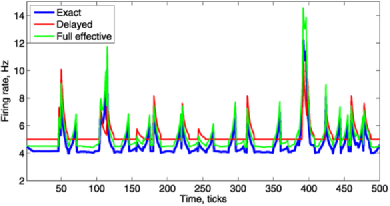
Figure 2: Quantifying the approximation accuracy of two spike train proposal densities. Blue trace: the true spiking rate $r_{i}(t)$ of one neuron conditioned on the spiking activity of all other neurons in a population of $N=50$ neurons; the rate is computed exactly via forward–backward procedure described in Section 2.3. A population of spontaneously spiking neurons with neurophysiologically feasible parameters (Section 2.7) was simulated for a total of $1$ sec at a time resolution of $\Delta=2$ msec. Approximate spiking rates obtained using just the delayed input, $J^{-}(t)$ [equation (6)], or full weak-coupling input, $\tilde{J}(t)$ [equation (2.4)], are shown in red and green, respectively. (In particular, the delayed input $J^{-}_{i}(t)$ and the full effective input $\tilde{J}_{i}(t)$ are computed as described in Section 2.4, and then we approximate the rates using $r_{i}(t)=f[J_{i}^{-}(t)]$ or $f[\tilde{J}_{i}(t)]$.) While the proposal based on the delayed inputs $J^{-}(t)$ reproduces the true spiking rate somewhat poorly, the weak-coupling $\tilde{J}(t)$ approximation is significantly more accurate.

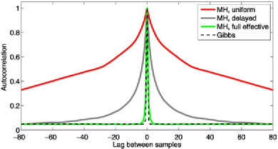
Figure 3: Autocorrelation functions for Gibbs and MH samplers. (The autocorrelation function is averaged over all time bins in the spike train.) Echoing the results of Figure 2, we see that the homogeneous (“uniform”) Poisson MH algorithm mixes slowly; the sampler based on the full weak-coupling input $\tilde{J}_{i}(t)$ mixes significantly more quickly than the sampler based on the delayed inputs $J^{-}_{i}(t)$. The standard Gibbs sampler performed about as well as the weak-coupling MH sampler. Simulation details are as in Figure 2, except a $10$ sec spike train was simulated here to collect a sufficient amount of data to distinguish the different algorithms.

Similar results are obtained when we apply the MH algorithm using these proposal densities (Figures 3 and 4). We use MH with $M=5\mbox{,}000$ samples for each proposal density, with a burn-in period of 1,000 samples, to obtain both the autocorrelation functions (Figure 3) and estimates for the instantaneous spiking rate $r_{i}(t)$ (Figure 4). We observe that the homogeneous Poisson proposal density leads to a very long autocorrelation scale, implying inefficient mixing, that is, long runs are necessary to obtain accurate estimates for quantities of interest such as $r_{i}(t)$. Indeed, we see in Figure 4 that 5,000 samples are insufficient to accurately reconstruct the desired rate $r_{i}(t)$. Similarly, for the proposal density based on the delayed inputs $J^{-}(t)$, the autocorrelation scale is shorter, but still in the range of 10–20 samples. The weak-coupling proposal, which incorporates information from both past and future observed spiking activity, mixes quite well, with an autocorrelation scale on the order of a single sample, and leads to an accurate reconstruction of the true rate in Figure 4. Interestingly, the simplest Gibbs sampling algorithm also performs well, with an autocorrelation length similar to that of the best MH sampler shown here.

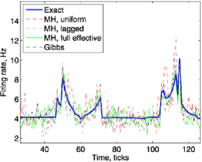
Figure 4: Comparing the accuracy of MH and Gibbs samplers. Each trace indicates the posterior spiking rate $r_{i}(t)$ for one hidden neuron, estimated from 5,000 samples using the Gibbs sampler and the three MH samplers compared in the preceding two figures. The results are similar: the homogeneous Poisson proposal performs badly [in the sense that the $r_{i}(t)$ computed based on these $5\mbox{,}000$ samples approximates the true $r_{i}(t)$ poorly], while the weak-coupling and Gibbs samplers outperform the sampler based on the delayed inputs $J^{-}_{i}(t)$ (in terms of variance around the true rate, computed via the full forward–backward HMM method, shown in blue). MH acceptance rates, $R$, varied from $R\approx 0.75$ for MH using the homogeneous Poisson proposal to $R\approx 0.98$ for MH using the proposal with full effective input $\tilde{J}_{i}(t)$. Simulation details are as in Figure 2. A shorter time interval of the simulated spike train is shown for greater clarity here.

We also study the performance of the weak-coupling proposal as a function of the strength of the interneuronal interactions in the network, and as a function of the number of neurons $N$ in the population and the length $T$ of the desired spike train (Figure 5). The acceptance rate falls at a rate approximately inverse to the coupling strength, which seems sensible, since this proposal is based on the approximation that the coupling strength is weak. We observe similar behavior with respect to the size of the neural population. In particular, the acceptance rate drops below $R\sim 0.1$ when $N\sim 600$–1,000. On the other hand, increasing the spike train length $T$ affects performance to only a moderate degree: even when the length of the sampled spike train is increased from $10$ sec to $160$ sec, the acceptance rate remains above $R\sim 0.4$.

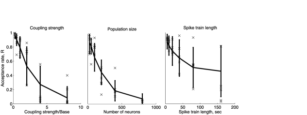
Figure 5: Acceptance rate of the weak-coupling MH algorithm as a function of coupling strength, $C$, neural population size, $N$, and spike length, $T$. We simulated sparsely connected networks of inhibitory and excitatory neurons as described in Section 2.7, with refractory effects up to $10$ msec long and interneural interactions up to $50$ msec long. Here a coupling strength value of $C=1$ corresponds to the neurobiologically motivated set of parameters in Section 2.7 (also in Figures 2–4); other values of $C$ corresponded to scaling $f(J(t))\rightarrow f(C\cdot J(t))$ in equation (2.1). $10$ sec of neural activity was simulated at a time resolution of $\Delta=2$ msec, with the neural population spiking at $\approx$4–5 Hz. 64 trials of 500 samples were simulated, with a new random neural network generated in each trial, from which we estimated $P(\mathbf{n}_{i}|\mathbf{n}_{\setminus i};\mathbf{w})$. Average acceptance rate $R$ and standard deviation are shown for such trials, as well as examples of several individual trials (“x”). MH algorithm performance degraded significantly as $C$ or $N$ increased. On the other hand, for larger values of $T$ performance degraded much less substantially, and even for the largest $T$ we examined ($160$ sec) the acceptance rate remained above $R\sim 0.4$.

One would expect that the performance of the MH algorithm in the case of more strongly-coupled neural networks can be improved by including strong short-term interaction and refractory effects explicitly into the proposal density. We discussed such an approach in Section 2.5. For weakly coupled networks, we expect the performance of this hybrid algorithm to be similar to that of our original proposal density; however, for more strongly coupled neural networks, we expect a better performance. This expectation is borne out in the simulations shown in Figure 6: the hybrid sampler (solid black line) performs significantly better than the original MH algorithm (dashed black line) and uniformly better than alternative hybrid strategies, for example, where only the short-scale truncated HMM is used, or where all interneural interactions are accounted for via the weak-coupling approximation, while the self-terms $w_{ii}$ are accounted for via a truncated HMM (gray lines). Similar results are obtained when we vary the size of the neural population $N$ (Figure 6).

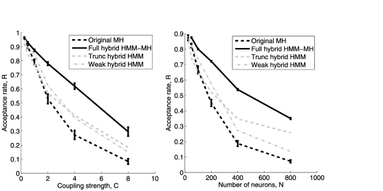
Figure 6: Acceptance rate of hybrid HMM-MH algorithm [equation (2.5)] as a function of the overall coupling strength $C$ and neural population size $N$. The hybrid algorithm (solid black line) performs substantially better than the original MH algorithm described in Section 2.4 (dashed black line), and uniformly better than alternative hybrid strategies, for example, where only a short-scale truncated HMM is used or where all interneural interactions are accounted for via weak-coupling approximation (gray lines). Simulations are as in Figure 5.

In the simulation settings described above (timestep $\Delta=2$ msec, with coupling currents $w_{ij}$ lasting up to $50$ ms) the MH algorithm (coded in Matlab without any particular algorithmic optimization) took $\approx$300–400 sec to produce 1,000 samples of 1,000 time-ticks each on a PC laptop (Intel Core Duo 2 GHz), dominated by the time necessary to produce 1,000 spike train proposals using the forward recursion. The hybrid algorithm had a similar computational complexity ($t_{\max}=10$ ms in the truncated HMM). The Gibbs algorithm had a somewhat higher computational cost, due largely to the fact that updates of the currents $J_{i}(t)$ for up to $50$ ms needed to be performed during each step, to decide whether to flip the state of each spike variable $n_{i}(t)$. This resulted in running times for the Gibbs sampler which were 5–20 times slower than for the MH sampler. The Gibbs updates are even slower in the calcium imaging setting (discussed at more length in the next section), due to the fact that each update requires us to update $C_{i}(t)$ over $n_{c}\tau^{c}_{i}$ timesteps (recall Section 2.6) for each proposed flip of $n_{i}(t)$.

3.1 Incorporating calcium fluorescence imaging observations

Next we examine the performance of the method we developed in Section 2.6 for sampling from $P(\mathbf{n}_{i}|\mathbf{n}_{\setminus i},\mathbf{F}_{i})$. We find that this sampler performs quite well in moderate and high SNR settings. More precisely, for values of eSNR greater than $\approx$5 [recall the definition of eSNR in equation (3)], the conditional distribution $P(\mathbf{n}_{i}|\mathbf{F}_{i})$ is localized near the true spike train quite effectively, leading to a high MH acceptance rate (Figures 7–9). Indeed, we find [as in Vogelstein et al. (2009)] that it is possible to achieve a sort of “super-resolution” in the sense that the MH algorithm can successfully return $P(\mathbf{n}_{i}|\mathbf{F}_{i})$ on the time-scale of $\Delta=2$ msec even when fluorescence observations are obtained at a much lower frame-rate (here $\mathit{FR}=50$ Hz).

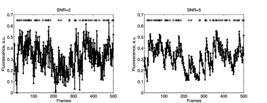
Figure 7: Example of observed fluorescence for low $\mathit{SNR}\approx 2$ and relatively high $\mathit{SNR}\approx 5$. $\Delta=2$ msec, and calcium imaging frame-rate $\mathit{FR}=50$ Hz. $10$ sec spike trains were simulated, with the neural population spiking at $\approx$4–5 Hz. Actual spikes of the target neuron are indicated with stars.

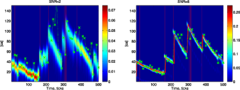
Figure 8: Example of $P(\mathbf{F}_{i}(t\dvtx T)|C_{i}(t))$ calculated as a $T$-mixture of Gaussians, as a function of time (x-axis) and $C_{i}(t)$ (y-axis); colorbar indicates the probability density at time $t$. For reference, true calcium concentration is shown in red, and “observed” calcium concentration at the imaging frames [i.e., $S^{-1}(F_{i}(t))$] is shown with green “x.” Simulation details are as in Figure 7, first second (50 frames) is shown for clarity. Time ticks correspond to $\Delta=2$ msec. Actual spike times of the target neuron are shown with red lines.

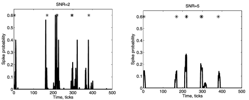
Figure 9: Posterior spike probability, $P(n_{i}(t)|\mathbf{n}_{\setminus i},\mathbf{F}_{i})$, estimated using MH algorithm. While the MH algorithm performs well for $\mathit{SNR}=5$ and above ($R\approx 0.8$), for low $\mathit{SNR}=2$ acceptance rate is only $R\approx 0.01$. Simulation details are as in Figure 7, first second (50 frames) is shown for clarity. Time ticks correspond to $\Delta=2$ msec. Actual spikes of the target neuron are shown with asterisks. Note that in the high-SNR case the sampler successfully recovers the smoothly-varying $P(n_{i}(t)|\mathbf{n}_{\setminus i},\mathbf{F}_{i})$ on a finer time-scale ($\Delta\approx 2$ msec) than the original fluorescence imaging data provided ($\Delta_{\mathit{FR}}\approx 20$ msec). However, in the low-SNR case the recovered firing rate is overly spiky and variable due to the slow mixing speed of the M-H chain; recall that similar behavior is visible in Figure 4.

Conversely, for low values of $e\mathit{SNR}$, for example, $e\mathit{SNR}\approx 1$, the backward density $P(\mathbf{F}_{i}(t\dvtx T)|n_{i}(t),C_{i}(t))$ becomes noninformative [i.e., relatively flat as a function of $n_{i}(t)$ and $C_{i}(t)$], and the acceptance rate of our MH algorithm reverts to the rate obtained under the conditions of no calcium imaging data. However, in the low-to-moderate SNR regime (e.g., $e\mathit{SNR}\approx 2$), the performance of the MH sampler can drop substantially. This is primarily due to deviations in the shape of $P(F_{i}(t)|C_{i}(t))$ from Gaussian at low SNR. Recall that we made several approximations in computing the backward density: first, this density is truly a mixture of ${\sim}2^{T-t}$ components, whereas we approximate it with a mixture of only ${\sim}T-t$ components. Second, we assume that each mixture component is Gaussian. Although the fluorescence $F_{i}(t)$ is described by normal statistics given the calcium variable $C_{i}(t)$, the relationship between the fluorescence mean and calcium transient can be nonlinear, and the variance may depend on $C_{i}(t)$ [recall equation (2.1)]. This makes the conditional distribution of $C_{i}(t)$ non-Gaussian in general, particularly at low-to-moderate levels of SNR (where the likelihood term is informative but not sufficiently sharp to justify a simple Laplace approximation). We tested the impact of each of these approximations individually by constructing a set of toy models where these different approximations were made exact; we found that the non-Gaussianity of $P(C_{i}(t)|F_{i}(t))$, due to nonlinear dependence of $F_{i}(t)$ on $C_{i}(t)$, was the primary factor responsible for the drop in performance. Thus, we expect that in cases where the saturating function $S(\cdot)$ is close to linear, the sampler should perform well across the full SNR range (Figure 10); in highly nonlinear settings, more sophisticated approximations [based on numerical integration techniques such as expectation propagation Minka (2001)] may be necessary, as discussed in the Conclusion section below. The MH sampler here took about twice as long as in the fully-observed spike train case discussed in the previous section, largely due to the increased complexity of the backward recursion described in Section 2.6.

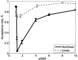
Figure 10: Acceptance rate of MH algorithms as a function of the calcium imaging effective SNR, equation (3). Calculations for two calcium signal models, with a toy linear (gray dashed) and realistic Hill (solid black) transfer function, $S(C_{i}(t))$, are shown. [See Vogelstein et al. (2009); Mishchenko, Vogelstein and Paninski (2011) for further details on the precise form of the nonlinear function $S(C_{i}(t))$; in this case, three or four spikes were sufficient to drive the calcium variable into a regime where the fluorescence signal was significantly saturated.] Performance of the MH algorithm is good both for high and low eSNR, but can suffer for intermediate $\mathit{eSNR}\approx 1.1$–3. This performance drop is primarily due to deviations of the conditional distribution $P(C_{i}(t)|F_{i}(t))$ from the Gaussian shape, as exemplified by the much better performance in the model where $S(\cdot)$ is linear and $P(C_{i}(t)|F_{i}(t))$ is thus Gaussian. Simulation details are as in Figure 7. For each eSNR 50 simulations for different neural populations were performed, and the average and standard error of these simulations are shown.

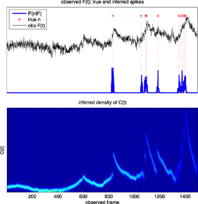
Figure 11: Application to real data (sample data courtesy of T. Sippy, R. Yuste, J. Vogelstein). Top: observed $F(t)$ (black) and true spike times (red) were recorded from a single neuron via simultaneous fluorescence imaging and intracellular patch-clamp electrophysiological recording; see Vogelstein et al. (2009) for further experimental details. Blue trace indicates posterior $P(n(t)|\mathbf{F})$ computed by the hybrid sampler. Bottom: $p(C(t)|\mathbf{F})$ computed by the hybrid sampler. Y-axis units are arbitrary in this case and have been suppressed. Note that the sampler infers spikes and jumps in $C(t)$ at the correct times.

Given the good performance of Gibbs sampling noted in the calcium-free setting discussed above, we also examined the Gibbs approach here. However, we found that the Gibbs algorithm was not able to procure the samples successfully given calcium imaging observations. In many cases we found that the Gibbs sampler converged rapidly to a particular spike train close to the truth, but would then become “stuck.” If initialized again, the sampler would often converge to a different spike train, close to the truth, only to become stuck again. This behavior is due to the fact that the conditional distributions $P(n_{i}(t)|\mathbf{n}_{i,\setminus t},\mathbf{F}_{i})$ can be quite sharply concentrated, leading to poor mixing between spike train configurations with high posterior probability; of course, this is a common problem with the Gibbs sampler (and indeed, this well-understood poor mixing behavior of the standard Gibbs chain is what led us to develop the more involved methods presented here in the first place). Roughly speaking, the extra constraints imposed by the fluorescence observations in $P(n_{i}(t)|\mathbf{n}_{i,\setminus t},\mathbf{F}_{i})$ relative to $P(n_{i}(t)|\mathbf{n}_{i,\setminus t})$ make the former distribution more “frustrated,” in physics language, making it harder for the Gibbs sampler to reach nearby states with high posterior probability and leading to the relatively slower Gibbs mixing rate in the calcium-imaging setting.

Finally, we applied the hybrid sampler to a sample of real calcium fluorescence imaging data (Figure 11), in which $F(t)$ and the true spike times $n(t)$ were recorded simultaneously. Thus, we have access to ground truth for $n(t)$ here, though of course only the observed fluorescence $\mathbf{F}$ is used to infer $p(n(t)|\mathbf{F})$. The model parameters were estimated using the EM method discussed in Vogelstein et al. (2009); again, only the observed $\mathbf{F}$ was used to infer the model parameters, not the true spike times $n(t)$. About $50$ spikes’ worth ($5\mbox{,}000$ fluorescence frames) of data was sufficient to adequately constrain the parameters. Then we applied the hybrid sampler using these parameters to the subset of data shown in Figure 11. The sampler does a good job of recovering the spike rate $n(t)$ from the observed fluorescence data $\mathbf{F}$, and seems to do a reasonable job of recovering the corresponding jumps in $p(C(t)|\mathbf{F})$ that occur at spike times. Note that we do not have access to the true intracellular calcium concentration $C(t)$, and therefore no ground truth comparisons are possible for this variable.

4 Conclusion

In this work we developed several Metropolis–Hastings approaches for sampling from the conditional distribution of neuronal spike trains, given either the activity of other neurons in the network or calcium-sensitive imaging observations. The most effective approach was the hybrid method described in Section 2.5, which takes advantage of the fact that strong short-term temporal dependencies within a single spike train may be handled via forward–backward hidden Markov model methods, while weaker long-term dependencies between neurons may be handled with the weak-coupling expansion developed in Section 2.4. In each case, to sample efficiently from the spike train at time $t$, it is important to incorporate not only past but also future information (i.e., spiking observations from times both before and after $t$); Pillow and Latham (2007) made a similar point. In the appendix we show that these methods may be extended rather easily to other exponential families (not just the Bernoulli and Poisson cases of most interest in the neuroscience setting); further applications to weakly-coupled Markov chains in nonneural settings seem worth exploring.

Two major avenues are open for future work. First, as noted in Figure 8, the proposed sampler suffers somewhat in the case of strongly nonlinear fluorescence observations, largely because in this case our mixture-of-Gaussians approximation of the backward density $P[\mathbf{F}_{i}(t\dvtx T)|C_{i}(t)]$ can break down. More sophisticated methods for approximating this density are available, and should be explored more thoroughly. Second, as discussed in Vogelstein et al. (2010), applications of these methods to real data are ongoing, via Monte Carlo-Expectation-Maximization methods similar to those discussed in Vogelstein et al. (2009); Mishchenko, Vogelstein and Paninski (2011), with the fast sampler introduced here replacing the slower Monte Carlo approaches discussed in Mishchenko, Vogelstein and Paninski (2011). Calcium-fluorescence imaging methods have exploded in popularity over the last several years, and we hope the methods presented here will prove useful in quantifying the cross-correlations and effective connectivity in neural populations observed via fluorescence imaging and multielectrode recording methods.

Appendix: Sampling from a weakly-coupled exponential family

As mentioned in Section 2.4, it is straightforward to develop a first-order proposal density in the weak-coupling limit more generally, in the case that the variables of interest are drawn from an exponential family distribution with linear sufficient statistics. We begin by writing down our exponential family model, using slightly more compact notation than in Section 2.4:

$$\log p(\{n_{it}\})=\sum_{it}f(J_{it})k(n_{it})+g(J_{it})+h(n_{it}),$$ (21)

with the coupling introduced via

$$J_{it}=b_{it}+\sum_{s>0,j}w^{ij}_{s}n_{j,t-s}.$$ (22)

As before, we may easily expand the joint log-density to the first order:

$$\log p(\{n_{it}\}) = \sum_{t}f(J_{it})k(n_{it})+g(J_{it})+h(n_{it})$$

$${}+\sum_{t,i\neq j}[f^{\prime}(b_{jt})k(n_{jt})+g^{\prime}(b_{jt})]\sum_{s>0}w_{s}^{ji}n_{i,t-s}$$

$${}+\mbox{const}(n_{it})+o(w).$$

Now if we introduce the assumption that the sufficient statistic is linear, that is, $k(n)=n$, then after rearranging the double sum over $s$ and $t$ we obtain

$$\log p(\{n_{it}\}) = \sum_{t}\biggl{[}f(J_{it})+\sum_{s>0,i\neq j}w_{s}^{ji}[f^{\prime}(b_{j,t+s})n_{j,t+s}+g^{\prime}(b_{j,t+s})]\biggr{]}n_{it}$$

$${}+h(n_{it})+\mbox{const}(n_{it})+o(w),$$

where again we have suppressed terms [such as $g(J_{it})$] which do not involve $n_{it}$; thus, to first order, the conditional distribution of $\{n_{it}\}$ given $\{n_{jt}\}$, $i\neq j$, remains within the same exponential family, but with a parameter shift

$$f(J_{it})\to f(J_{it})+\sum_{s>0,i\neq j}w_{s}^{ji}[f^{\prime}(b_{j,t+s})n_{j,t+s}+g^{\prime}(b_{j,t+s})].$$ (25)

In the canonical parameterization, $f(J)=J$, standard exponential family theory [Casella and Berger (2001)] shows that $g^{\prime}(b_{j,t+s})=-E(n_{j,t+s}|b_{j,t+s})$, and the parameter shift simplifies to

$$J_{it}\to J_{it}+\sum_{s>0,i\neq j}w_{s}^{ij}[n_{j,t+s}-E(n_{j,t+s}|b_{j,t+s})].$$ (26)

See Beck et al. (2007) for a discussion of some related results.

As a concrete example, consider the Gaussian case:

$$\log p(\{n_{it}\})=-\sum_{it}\frac{1}{2\sigma^{2}_{i}}(n_{it}-J_{it})^{2}+\mbox{const.},$$ (27)

with $J_{it}$ as above. In this case we may define $f_{i}(J_{it})=J_{it}/\sigma^{2}_{i}$ and $g_{i}(J_{it})=-J_{it}^{2}/2\sigma^{2}_{i}$; thus, we find that the parameter shift in this case is

$$f(J_{it})=\frac{J_{it}}{\sigma^{2}_{i}}\to\frac{J_{it}}{\sigma^{2}_{i}}+\sum_{s>0,i\neq j}\frac{w_{s}^{ij}}{\sigma^{2}_{j}}[n_{j,t+s}-b_{j,t+s}].$$ (28)

In this linear-Gaussian case, we may compute the exact conditional distribution of $n_{i}$ via the usual Gaussian conditioning formula; the necessary covariance and inverse covariance matrices may be obtained via standard AR model computations. It is straightforward to check that this exact formula agrees with equation (28) up to $o(w)$ terms in the small-$w$ limit.

References

- Abeles (1991) {bbook}[auto:STB—2011-03-03—12:04:44] \bauthor\bsnmAbeles, \bfnmM.\binitsM. (\byear1991). \btitleCorticonics. \bpublisherCambridge Univ. Press, \baddressCambridge. \endbibitem
- Beck et al. (2007) {barticle}[pbm] \bauthor\bsnmBeck, \bfnmJ.\binitsJ., \bauthor\bsnmMa, \bfnmW. J.\binitsW. J., \bauthor\bsnmLatham, \bfnmP. E.\binitsP. E. and \bauthor\bsnmPouget, \bfnmA.\binitsA. (\byear2007). \btitleProbabilistic population codes and the exponential family of distributions. \bjournalProg. Brain Res. \bvolume165 \bpages509–519. \biddoi=10.1016/S0079-6123(06)65032-2, issn=0079-6123, pii=S0079-6123(06)65032-2, pmid=17925267 \endbibitem
- Bohland et al. (2009) {bmisc}[auto:STB—2011-03-03—12:04:44] \bauthor\bsnmBohland, \bfnmJ.\binitsJ. \betalet al. (\byear2009). \bhowpublishedA proposal for a coordinated effort for the determination of brainwide neuroanatomical connectivity in model organisms at a mesoscopic scale. Available at ArXiv:0901.4598. \endbibitem
- Braitenberg and Schuz (1998) {bbook}[auto:STB—2011-03-03—12:04:44] \bauthor\bsnmBraitenberg, \bfnmV.\binitsV. and \bauthor\bsnmSchuz, \bfnmA.\binitsA. (\byear1998). \btitleCortex: Statistics and Geometry of Neuronal Connectivity. \bpublisherSpringer, \baddressBerlin. \endbibitem
- Briggman and Denk (2006) {barticle}[auto:STB—2011-03-03—12:04:44] \bauthor\bsnmBriggman, \bfnmK. L.\binitsK. L. and \bauthor\bsnmDenk, \bfnmW.\binitsW. (\byear2006). \btitleTowards neural circuit reconstruction with volume electron microscopy techniques. \bjournalCurrent Opinions in Neurobiology \bvolume16 \bpages562. \endbibitem
- Brillinger (1988) {barticle}[auto:STB—2011-03-03—12:04:44] \bauthor\bsnmBrillinger, \bfnmD.\binitsD. (\byear1988). \btitleMaximum likelihood analysis of spike trains of interacting nerve cells. \bjournalBiological Cyberkinetics \bvolume59 \bpages189–200. \endbibitem
- Brillinger (1992) {barticle}[auto:STB—2011-03-03—12:04:44] \bauthor\bsnmBrillinger, \bfnmD.\binitsD. (\byear1992). \btitleNerve cell spike train data analysis: A progression of technique. \bjournalJ. Amer. Statist. Assoc. \bvolume87 \bpages260–271. \endbibitem
- Bureau, Shepherd and Svoboda (2004) {barticle}[pbm] \bauthor\bsnmBureau, \bfnmIngrid\binitsI., \bauthor\bsnmShepherd, \bfnmGordon M G\binitsG. M. G. and \bauthor\bsnmSvoboda, \bfnmKarel\binitsK. (\byear2004). \btitlePrecise development of functional and anatomical columns in the neocortex. \bjournalNeuron \bvolume42 \bpages789–801. \biddoi=10.1016/j.neuron.2004.05.002, issn=0896-6273, pii=S0896627304002910, pmid=15182718 \endbibitem
- Casella and Berger (2001) {bbook}[auto:STB—2011-03-03—12:04:44] \bauthor\bsnmCasella, \bfnmG.\binitsG. and \bauthor\bsnmBerger, \bfnmR.\binitsR. (\byear2001). \btitleStatistical Inference. \bpublisherDuxbury Press. \endbibitem
- Chornoboy, Schramm and Karr (1988) {barticle}[mr] \bauthor\bsnmChornoboy, \bfnmE. S.\binitsE. S., \bauthor\bsnmSchramm, \bfnmL. P.\binitsL. P. and \bauthor\bsnmKarr, \bfnmA. F.\binitsA. F. (\byear1988). \btitleMaximum likelihood identification of neural point process systems. \bjournalBiol. Cybernet. \bvolume59 \bpages265–275. \biddoi=10.1007/BF00332915, issn=0340-1200, mr=0961117 \endbibitem
- Cossart, Aronov and Yuste (2003) {barticle}[pbm] \bauthor\bsnmCossart, \bfnmRosa\binitsR., \bauthor\bsnmAronov, \bfnmDmitriy\binitsD. and \bauthor\bsnmYuste, \bfnmRafael\binitsR. (\byear2003). \btitleAttractor dynamics of network UP states in the neocortex. \bjournalNature \bvolume423 \bpages283–288. \biddoi=10.1038/nature01614, issn=0028-0836, pii=nature01614, pmid=12748641 \endbibitem
- De Gunst, Künsch and Schouten (2001) {barticle}[mr] \bauthor\bsnmDe Gunst, \bfnmM. C. M.\binitsM. C. M., \bauthor\bsnmKünsch, \bfnmH. R.\binitsH. R. and \bauthor\bsnmSchouten, \bfnmJ. G.\binitsJ. G. (\byear2001). \btitleStatistical analysis of ion channel data using hidden Markov models with correlated state-dependent noise and filtering. \bjournalJ. Amer. Statist. Assoc. \bvolume96 \bpages805–815. \biddoi=10.1198/016214501753208519, issn=0162-1459, mr=1946357 \endbibitem
- Escola et al. (2011) {bmisc}[auto:STB—2011-03-03—12:04:44] \bauthor\bsnmEscola, \bfnmS.\binitsS., \bauthor\bsnmFontanini, \bfnmA.\binitsA., \bauthor\bsnmKatz, \bfnmD.\binitsD. and \bauthor\bsnmPaninski, \bfnmL.\binitsL. (\byear2011). \bhowpublishedHidden Markov models for the stimulus-response relationships of multi-state neural systems. Neural Computation. To appear. \endbibitem
- Gómez-Urquijo et al. (2000) {barticle}[pbm] \bauthor\bsnmGómez-Urquijo, \bfnmS. M.\binitsS. M., \bauthor\bsnmReblet, \bfnmC.\binitsC., \bauthor\bsnmBueno-López, \bfnmJ. L.\binitsJ. L. and \bauthor\bsnmGutiérrez-Ibarluzea, \bfnmI.\binitsI. (\byear2000). \btitleGABAergic neurons in the rabbit visual cortex: Percentage, layer distribution and cortical projections. \bjournalBrain Res. \bvolume862 \bpages171–179. \bidissn=0006-8993, pii=S0006-8993(00)02114-4, pmid=10799682 \endbibitem
- Hagmann et al. (2007) {barticle}[pbm] \bauthor\bsnmHagmann, \bfnmPatric\binitsP., \bauthor\bsnmKurant, \bfnmMaciej\binitsM., \bauthor\bsnmGigandet, \bfnmXavier\binitsX., \bauthor\bsnmThiran, \bfnmPatrick\binitsP., \bauthor\bsnmWedeen, \bfnmVan J.\binitsV. J., \bauthor\bsnmMeuli, \bfnmReto\binitsR. and \bauthor\bsnmThiran, \bfnmJean-Philippe\binitsJ.-P. (\byear2007). \btitleMapping human whole-brain structural networks with diffusion MRI. \bjournalPLoS ONE \bvolume2 \bpagese597. \biddoi=10.1371/journal.pone.0000597, issn=1932-6203, pmcid=1895920, pmid=17611629 \endbibitem
- Hagmann et al. (2008) {barticle}[pbm] \bauthor\bsnmHagmann, \bfnmPatric\binitsP., \bauthor\bsnmCammoun, \bfnmLeila\binitsL., \bauthor\bsnmGigandet, \bfnmXavier\binitsX., \bauthor\bsnmMeuli, \bfnmReto\binitsR., \bauthor\bsnmHoney, \bfnmChristopher J.\binitsC. J., \bauthor\bsnmWedeen, \bfnmVan J.\binitsV. J. and \bauthor\bsnmSporns, \bfnmOlaf\binitsO. (\byear2008). \btitleMapping the structural core of human cerebral cortex. \bjournalPLoS Biol. \bvolume6 \bpagese159. \biddoi=10.1371/journal.pbio.0060159, issn=1545-7885, pii=07-PLBI-RA-4028, pmcid=2443193, pmid=18597554 \endbibitem
- Harris et al. (2003) {barticle}[pbm] \bauthor\bsnmHarris, \bfnmKenneth D.\binitsK. D., \bauthor\bsnmCsicsvari, \bfnmJozsef\binitsJ., \bauthor\bsnmHirase, \bfnmHajime\binitsH., \bauthor\bsnmDragoi, \bfnmGeorge\binitsG. and \bauthor\bsnmBuzsáki, \bfnmGyörgy\binitsG. (\byear2003). \btitleOrganization of cell assemblies in the hippocampus. \bjournalNature \bvolume424 \bpages552–556. \biddoi=10.1038/nature01834, issn=1476-4687, pii=nature01834, pmid=12891358 \endbibitem
- Hatsopoulos et al. (1998) {barticle}[pbm] \bauthor\bsnmHatsopoulos, \bfnmN. G.\binitsN. G., \bauthor\bsnmOjakangas, \bfnmC. L.\binitsC. L., \bauthor\bsnmPaninski, \bfnmL.\binitsL. and \bauthor\bsnmDonoghue, \bfnmJ. P.\binitsJ. P. (\byear1998). \btitleInformation about movement direction obtained from synchronous activity of motor cortical neurons. \bjournalProc. Natl. Acad. Sci. USA \bvolume95 \bpages15706–15711. \bidissn=0027-8424, pmcid=28108, pmid=9861034 \endbibitem
- Helmstaedter, Briggman and Denk (2009) {bmisc}[auto:STB—2011-03-03—12:04:44] \bauthor\bsnmHelmstaedter, \bfnmM.\binitsM., \bauthor\bsnmBriggman, \bfnmK. L.\binitsK. L. and \bauthor\bsnmDenk, \bfnmW.\binitsW. (\byear2009). \bhowpublished3d structural imaging of the brain with photons and electrons. Current Opinions in Neurobiology. Page Epub. \endbibitem
- Jordan (1999) {bbook}[auto:STB—2011-03-03—12:04:44] \bauthor\bsnmJordan, \bfnmM. I.\binitsM. I. (\byear1999). \btitleLearning in Graphical Models. \bpublisherMIT Press, \baddressCambridge, MA. \endbibitem
- Kulkarni and Paninski (2007) {barticle}[auto:STB—2011-03-03—12:04:44] \bauthor\bsnmKulkarni, \bfnmJ.\binitsJ. and \bauthor\bsnmPaninski, \bfnmL.\binitsL. (\byear2007). \btitleCommon-input models for multiple neural spike-train data. \bjournalNetwork: Computation in Neural Systems \bvolume18 \bpages375–407. \endbibitem
- Lefort, Tomm and Sarria (2009) {barticle}[auto:STB—2011-03-03—12:04:44] \bauthor\bsnmLefort, \bfnmS.\binitsS., \bauthor\bsnmTomm, \bfnmC.\binitsC. \bauthor\bsnmFloyd Sarria, \bfnmJ.-C.\binitsJ.-C. and \bauthor\bsnmPetersen, \bfnmC. C. H.\binitsC. C. H. (\byear2009). \btitleThe excitatory neuronal network of the c2 barrel column in mouse primary somatosensory cortex. \bjournalNeuron \bvolume61 \bpages301–316. \endbibitem
- Luczak et al. (2007) {barticle}[pbm] \bauthor\bsnmLuczak, \bfnmArtur\binitsA., \bauthor\bsnmBarthó, \bfnmPeter\binitsP., \bauthor\bsnmMarguet, \bfnmStephan L.\binitsS. L., \bauthor\bsnmBuzsáki, \bfnmGyörgy\binitsG. and \bauthor\bsnmHarris, \bfnmKenneth D.\binitsK. D. (\byear2007). \btitleSequential structure of neocortical spontaneous activity in vivo. \bjournalProc. Natl. Acad. Sci. USA \bvolume104 \bpages347–352. \biddoi=10.1073/pnas.0605643104, issn=0027-8424, pii=0605643104, pmcid=1765463, pmid=17185420 \endbibitem
- Luo, Callaway and Svoboda (2008) {barticle}[pbm] \bauthor\bsnmLuo, \bfnmLiqun\binitsL., \bauthor\bsnmCallaway, \bfnmEdward M.\binitsE. M. and \bauthor\bsnmSvoboda, \bfnmKarel\binitsK. (\byear2008). \btitleGenetic dissection of neural circuits. \bjournalNeuron \bvolume57 \bpages634–660. \biddoi=10.1016/j.neuron.2008.01.002, issn=1097-4199, mid=NIHMS87357, pii=S0896-6273(08)00031-7, pmcid=2628815, pmid=18341986 \endbibitem
- Minka (2001) {bmisc}[mr] \bauthor\bsnmMinka, \bfnmThomas P.\binitsT. P. (\byear2001). \bhowpublishedA family of algorithms for approximate Bayesian inference. Ph.D. thesis, Massachusetts Institute of Technology. \bidmr=2717007 \endbibitem
- Mishchenko, Vogelstein and Paninski (2011) {bmisc}[auto:STB—2011-03-03—12:04:44] \bauthor\bsnmMishchenko, \bfnmY.\binitsY., \bauthor\bsnmVogelstein, \bfnmJ.\binitsJ. and \bauthor\bsnmPaninski, \bfnmL.\binitsL. (\byear2011). \bhowpublishedA bayesian approach for inferring neuronal connectivity from calcium fluorescent imaging data. Ann. Appl. Stat. To appear. \endbibitem
- Neal, Beal and Roweis (2003) {bmisc}[auto:STB—2011-03-03—12:04:44] \bauthor\bsnmNeal, \bfnmR.\binitsR., \bauthor\bsnmBeal, \bfnmM.\binitsM. and \bauthor\bsnmRoweis, \bfnmS.\binitsS. (\byear2003). \bhowpublishedInferring state sequences for non-linear systems with embedded hidden Markov models. NIPS 16. \endbibitem
- Nykamp (2003) {bmisc}[auto:STB—2011-03-03—12:04:44] \bauthor\bsnmNykamp, \bfnmD.\binitsD. (\byear2003). \bhowpublishedReconstructing stimulus-driven neural networks from spike times. NIPS 15 309–316. \endbibitem
- Nykamp (2005a) {barticle}[mr] \bauthor\bsnmNykamp, \bfnmDuane Q.\binitsD. Q. (\byear2005a). \btitleRevealing pairwise coupling in linear-nonlinear networks. \bjournalSIAM J. Appl. Math. \bvolume65 \bpages2005–2032 (electronic). \biddoi=10.1137/S0036139903437072, issn=0036-1399, mr=2177736 \endbibitem
- Nykamp (2005b) {barticle}[mr] \bauthor\bsnmNykamp, \bfnmDuane Q.\binitsD. Q. (\byear2005b). \btitleRevealing pairwise coupling in linear-nonlinear networks. \bjournalSIAM J. Appl. Math. \bvolume65 \bpages2005–2032 (electronic). \biddoi=10.1137/S0036139903437072, issn=0036-1399, mr=2177736 \endbibitem
- Nykamp (2007) {barticle}[mr] \bauthor\bsnmNykamp, \bfnmDuane Q.\binitsD. Q. (\byear2007). \btitleA mathematical framework for inferring connectivity in probabilistic neuronal networks. \bjournalMath. Biosci. \bvolume205 \bpages204–251. \biddoi=10.1016/j.mbs.2006.08.020, issn=0025-5564, mr=2295044 \endbibitem
- Ohki et al. (2005) {barticle}[auto:STB—2011-03-03—12:04:44] \bauthor\bsnmOhki, \bfnmK.\binitsK., \bauthor\bsnmChung, \bfnmS.\binitsS., \bauthor\bsnmCh’ng, \bfnmY.\binitsY., \bauthor\bsnmKara, \bfnmP.\binitsP. and \bauthor\bsnmReid, \bfnmC.\binitsC. (\byear2005). \btitleFunctional imaging with cellular resolution reveals precise micro-architecture in visual cortex. \bjournalNature \bvolume433 \bpages597–603. \endbibitem
- Okatan, Wilson and Brown (2005) {barticle}[pbm] \bauthor\bsnmOkatan, \bfnmMurat\binitsM., \bauthor\bsnmWilson, \bfnmMatthew A.\binitsM. A. and \bauthor\bsnmBrown, \bfnmEmery N.\binitsE. N. (\byear2005). \btitleAnalyzing functional connectivity using a network likelihood model of ensemble neural spiking activity. \bjournalNeural Comput. \bvolume17 \bpages1927–1961. \biddoi=10.1162/0899766054322973, issn=0899-7667, pmid=15992486 \endbibitem
- Paninski (2004) {barticle}[auto:STB—2011-03-03—12:04:44] \bauthor\bsnmPaninski, \bfnmL.\binitsL. (\byear2004). \btitleMaximum likelihood estimation of cascade point-process neural encoding models. \bjournalNetwork: Computation in Neural Systems \bvolume15 \bpages243–262. \endbibitem
- Paninski et al. (2004) {barticle}[pbm] \bauthor\bsnmPaninski, \bfnmLiam\binitsL., \bauthor\bsnmShoham, \bfnmShy\binitsS., \bauthor\bsnmFellows, \bfnmMatthew R.\binitsM. R., \bauthor\bsnmHatsopoulos, \bfnmNicholas G.\binitsN. G. and \bauthor\bsnmDonoghue, \bfnmJohn P.\binitsJ. P. (\byear2004). \btitleSuperlinear population encoding of dynamic hand trajectory in primary motor cortex. \bjournalJ. Neurosci. \bvolume24 \bpages8551–8561. \biddoi=10.1523/JNEUROSCI.0919-04.2004, issn=1529-2401, pii=24/39/8551, pmid=15456829 \endbibitem
- Petreanu et al. (2009) {barticle}[pbm] \bauthor\bsnmPetreanu, \bfnmLeopoldo\binitsL., \bauthor\bsnmMao, \bfnmTianyi\binitsT., \bauthor\bsnmSternson, \bfnmScott M.\binitsS. M. and \bauthor\bsnmSvoboda, \bfnmKarel\binitsK. (\byear2009). \btitleThe subcellular organization of neocortical excitatory connections. \bjournalNature \bvolume457 \bpages1142–1145. \biddoi=10.1038/nature07709, issn=1476-4687, mid=HHMIMS143295, pii=nature07709, pmcid=2745650, pmid=19151697 \endbibitem
- Pillow and Latham (2007) {bmisc}[auto:STB—2011-03-03—12:04:44] \bauthor\bsnmPillow, \bfnmJ.\binitsJ. and \bauthor\bsnmLatham, \bfnmP.\binitsP. (\byear2007). \bhowpublishedNeural characterization in partially observed populations of spiking neurons. NIPS. \endbibitem
- Pillow et al. (2008) {barticle}[auto:STB—2011-03-03—12:04:44] \bauthor\bsnmPillow, \bfnmJ.\binitsJ., \bauthor\bsnmShlens, \bfnmJ.\binitsJ., \bauthor\bsnmPaninski, \bfnmL.\binitsL., \bauthor\bsnmSher, \bfnmA.\binitsA., \bauthor\bsnmLitke, \bfnmA.\binitsA., \bauthor\bsnmChichilnisky, \bfnmE.\binitsE. and \bauthor\bsnmSimoncelli, \bfnmE.\binitsE. (\byear2008). \btitleSpatiotemporal correlations and visual signaling in a complete neuronal population. \bjournalNature \bvolume454 \bpages995–999. \endbibitem
- Plesser and Gerstner (2000) {barticle}[pbm] \bauthor\bsnmPlesser, \bfnmH. E.\binitsH. E. and \bauthor\bsnmGerstner, \bfnmW.\binitsW. (\byear2000). \btitleNoise in integrate-and-fire neurons: From stochastic input to escape rates. \bjournalNeural Comput. \bvolume12 \bpages367–384. \bidissn=0899-7667, pmid=10636947 \endbibitem
- Rabiner (1989) {barticle}[auto:STB—2011-03-03—12:04:44] \bauthor\bsnmRabiner, \bfnmL. R.\binitsL. R. (\byear1989). \btitleA tutorial on hidden Markov models and selected applications in speech recognition. \bjournalProceedings of the IEEE \bvolume72 \bpages257–286. \endbibitem
- Rigat, de Gunst and van Pelt (2006) {barticle}[mr] \bauthor\bsnmRigat, \bfnmFabio\binitsF., \bauthor\bparticlede \bsnmGunst, \bfnmMathisca\binitsM. and \bauthor\bparticlevan \bsnmPelt, \bfnmJaap\binitsJ. (\byear2006). \btitleBayesian modelling and analysis of spatio-temporal neuronal networks. \bjournalBayesian Anal. \bvolume1 \bpages733–764 (electronic). \bidissn=1931-6690, mr=2282205 \endbibitem
- Santhanam et al. (2006) {barticle}[pbm] \bauthor\bsnmSanthanam, \bfnmGopal\binitsG., \bauthor\bsnmRyu, \bfnmStephen I.\binitsS. I., \bauthor\bsnmYu, \bfnmByron M.\binitsB. M., \bauthor\bsnmAfshar, \bfnmAfsheen\binitsA. and \bauthor\bsnmShenoy, \bfnmKrishna V.\binitsK. V. (\byear2006). \btitleA high-performance brain-computer interface. \bjournalNature \bvolume442 \bpages195–198. \biddoi=10.1038/nature04968, issn=1476-4687, pii=nature04968, pmid=16838020 \endbibitem
- Sato et al. (2007) {barticle}[pbm] \bauthor\bsnmSato, \bfnmTakashi R.\binitsT. R., \bauthor\bsnmGray, \bfnmNoah W.\binitsN. W., \bauthor\bsnmMainen, \bfnmZachary F.\binitsZ. F. and \bauthor\bsnmSvoboda, \bfnmKarel\binitsK. (\byear2007). \btitleThe functional microarchitecture of the mouse barrel cortex. \bjournalPLoS Biol. \bvolume5 \bpagese189. \biddoi=10.1371/journal.pbio.0050189, issn=1545-7885, pii=06-PLBI-RA-2351, pmcid=1914403, pmid=17622195 \endbibitem
- Sayer, Friedlander and Redman (1990) {barticle}[pbm] \bauthor\bsnmSayer, \bfnmR. J.\binitsR. J., \bauthor\bsnmFriedlander, \bfnmM. J.\binitsM. J. and \bauthor\bsnmRedman, \bfnmS. J.\binitsS. J. (\byear1990). \btitleThe time course and amplitude of EPSPs evoked at synapses between pairs of CA3/CA1 neurons in the hippocampal slice. \bjournalJ. Neurosci. \bvolume10 \bpages826–836. \bidissn=0270-6474, pmid=2319304 \endbibitem
- Shepherd, Pologruto and Svoboda (2003) {barticle}[pbm] \bauthor\bsnmShepherd, \bfnmGordon M G\binitsG. M. G., \bauthor\bsnmPologruto, \bfnmThomas A.\binitsT. A. and \bauthor\bsnmSvoboda, \bfnmKarel\binitsK. (\byear2003). \btitleCircuit analysis of experience-dependent plasticity in the developing rat barrel cortex. \bjournalNeuron \bvolume38 \bpages277–289. \bidissn=0896-6273, pii=S0896627303001521, pmid=12718861 \endbibitem
- Smith (2007) {barticle}[auto:STB—2011-03-03—12:04:44] \bauthor\bsnmSmith, \bfnmS. J.\binitsS. J. (\byear2007). \btitleCircuit reconstruction tools today. \bjournalCurr. Opin. Neurobiol. \bvolume17 \bpages601–608. \endbibitem
- Smith and Brown (2003) {barticle}[pbm] \bauthor\bsnmSmith, \bfnmAnne C.\binitsA. C. and \bauthor\bsnmBrown, \bfnmEmery N.\binitsE. N. (\byear2003). \btitleEstimating a state-space model from point process observations. \bjournalNeural Comput. \bvolume15 \bpages965–991. \biddoi=10.1162/089976603765202622, issn=0899-7667, pmid=12803953 \endbibitem
- Song et al. (2005) {barticle}[auto:STB—2011-03-03—12:04:44] \bauthor\bsnmSong, \bfnmS.\binitsS., \bauthor\bsnmSjostrom, \bfnmP. J.\binitsP. J., \bauthor\bsnmReiql, \bfnmM.\binitsM., \bauthor\bsnmNelson, \bfnmS.\binitsS. and \bauthor\bsnmChklovskii, \bfnmD. B.\binitsD. B. (\byear2005). \btitleHighly nonrandom features of synaptic connectivity in local cortical circuits. \bjournalPLoS Biology \bvolume3 \bpagese68. \endbibitem
- Srinivasan et al. (2006) {barticle}[mr] \bauthor\bsnmSrinivasan, \bfnmLakshminarayan\binitsL., \bauthor\bsnmEden, \bfnmUri T.\binitsU. T., \bauthor\bsnmWillsky, \bfnmAlan S.\binitsA. S. and \bauthor\bsnmBrown, \bfnmEmery N.\binitsE. N. (\byear2006). \btitleA state-space analysis for reconstruction of goal-directed movements using neural signals. \bjournalNeural Comput. \bvolume18 \bpages2465–2494. \biddoi=10.1162/neco.2006.18.10.2465, issn=0899-7667, mr=2256113 \endbibitem
- Stein et al. (2004) {barticle}[auto:STB—2011-03-03—12:04:44] \bauthor\bsnmStein, \bfnmR. B.\binitsR. B., \bauthor\bsnmWeber, \bfnmD. J.\binitsD. J., \bauthor\bsnmAoyagi, \bfnmY.\binitsY., \bauthor\bsnmProchazka, \bfnmA.\binitsA., \bauthor\bsnmWagenaar, \bfnmJ. B. M.\binitsJ. B. M., \bauthor\bsnmShoham, \bfnmS.\binitsS. and \bauthor\bsnmNormann, \bfnmR. A.\binitsR. A. (\byear2004). \btitleCoding of position by simultaneously recorded sensory neurones in the cat dorsal root ganglion. \bjournalJ. Physiol. (Lond.) \bvolume560 \bpages883–896. \endbibitem
- Stevenson et al. (2009) {barticle}[auto:STB—2011-03-03—12:04:44] \bauthor\bsnmStevenson, \bfnmI. H.\binitsI. H., \bauthor\bsnmRebesco, \bfnmJ. M.\binitsJ. M., \bauthor\bsnmHatsopoulos, \bfnmN. G.\binitsN. G., \bauthor\bsnmHaga, \bfnmZ.\binitsZ., \bauthor\bsnmMiller, \bfnmL. E.\binitsL. E. and \bauthor\bsnmKording, \bfnmK. P.\binitsK. P. (\byear2009). \btitleBayesian inference of functional connectivity and network structure from spikes. \bjournalIEEE Trans. Neural Systems and Rehab. \bvolume17 \bpages203–213. \endbibitem
- Toyoizumi, Rahnama Rad and Paninski (2009) {barticle}[mr] \bauthor\bsnmToyoizumi, \bfnmTaro\binitsT., \bauthor\bsnmRahnama Rad, \bfnmKamiar\binitsK. and \bauthor\bsnmPaninski, \bfnmLiam\binitsL. (\byear2009). \btitleMean-field approximations for coupled populations of generalized linear model spiking neurons with Markov refractoriness. \bjournalNeural Comput. \bvolume21 \bpages1203–1243. \biddoi=10.1162/neco.2008.04-08-757, issn=0899-7667, mr=2514667 \endbibitem
- Truccolo et al. (2005) {barticle}[pbm] \bauthor\bsnmTruccolo, \bfnmWilson\binitsW., \bauthor\bsnmEden, \bfnmUri T.\binitsU. T., \bauthor\bsnmFellows, \bfnmMatthew R.\binitsM. R., \bauthor\bsnmDonoghue, \bfnmJohn P.\binitsJ. P. and \bauthor\bsnmBrown, \bfnmEmery N.\binitsE. N. (\byear2005). \btitleA point process framework for relating neural spiking activity to spiking history, neural ensemble, and extrinsic covariate effects. \bjournalJ. Neurophysiol. \bvolume93 \bpages1074–1089. \biddoi=10.1152/jn.00697.2004, issn=0022-3077, pii=00697.2004, pmid=15356183 \endbibitem
- Tsien (1989) {barticle}[pbm] \bauthor\bsnmTsien, \bfnmR. Y.\binitsR. Y. (\byear1989). \btitleFluorescent probes of cell signaling. \bjournalAnnu. Rev. Neurosci. \bvolume12 \bpages227–253. \biddoi=10.1146/annurev.ne.12.030189.001303, issn=0147-006X, pmid=2648950 \endbibitem
- Vakorin, Krakovska and McIntosh (2009) {barticle}[pbm] \bauthor\bsnmVakorin, \bfnmVasily A.\binitsV. A., \bauthor\bsnmKrakovska, \bfnmOlga A.\binitsO. A. and \bauthor\bsnmMcIntosh, \bfnmAnthony R.\binitsA. R. (\byear2009). \btitleConfounding effects of indirect connections on causality estimation. \bjournalJ. Neurosci. Methods \bvolume184 \bpages152–160. \biddoi=10.1016/j.jneumeth.2009.07.014, issn=1872-678X, pii=S0165-0270(09)00390-2, pmid=19628006 \endbibitem
- Vidne et al. (2009) {bmisc}[auto:STB—2011-03-03—12:04:44] \bauthor\bsnmVidne, \bfnmM.\binitsM., \bauthor\bsnmKulkarni, \bfnmJ.\binitsJ., \bauthor\bsnmAhmadian, \bfnmY.\binitsY., \bauthor\bsnmPillow, \bfnmJ.\binitsJ., \bauthor\bsnmShlens, \bfnmJ.\binitsJ., \bauthor\bsnmChichilnisky, \bfnmE.\binitsE., \bauthor\bsnmSimoncelli, \bfnmE.\binitsE. and \bauthor\bsnmPaninski, \bfnmL.\binitsL. (\byear2009). \bhowpublishedInferring functional connectivity in an ensemble of retinal ganglion cells sharing a common input. Abstract. In Computational and Systems Neuroscience 2009 Meeting. DOI:10.3389/conf.neuro.06.2009.03.248. \endbibitem
- Vogelstein et al. (2010) {bmisc}[auto:STB—2011-03-03—12:04:44] \bauthor\bsnmVogelstein, \bfnmJ.\binitsJ., \bauthor\bsnmMachado, \bfnmT.\binitsT., \bauthor\bsnmMishchenko, \bfnmY.\binitsY., \bauthor\bsnmPacker, \bfnmA.\binitsA., \bauthor\bsnmYuste, \bfnmR.\binitsR. and \bauthor\bsnmPaninski, \bfnmL.\binitsL. (\byear2010). \bhowpublishedMethods for neural circuit inference from population calcium imaging data. Abstract. In Computational and Systems Neuroscience 2010 Meeting. DOI:10.3389/conf.fnins.2010.03. 00176. \endbibitem
- Vogelstein et al. (2009) {barticle}[pbm] \bauthor\bsnmVogelstein, \bfnmJoshua T.\binitsJ. T., \bauthor\bsnmWatson, \bfnmBrendon O.\binitsB. O., \bauthor\bsnmPacker, \bfnmAdam M.\binitsA. M., \bauthor\bsnmYuste, \bfnmRafael\binitsR., \bauthor\bsnmJedynak, \bfnmBruno\binitsB. and \bauthor\bsnmPaninski, \bfnmLiam\binitsL. (\byear2009). \btitleSpike inference from calcium imaging using sequential Monte Carlo methods. \bjournalBiophys. J. \bvolume97 \bpages636–655. \biddoi=10.1016/j.bpj.2008.08.005, issn=1542-0086, pii=S0006-3495(09)00311-7, pmcid=2711341, pmid=19619479 \endbibitem
- Yasuda et al. (2004) {barticle}[auto:STB—2011-03-03—12:04:44] \bauthor\bsnmYasuda, \bfnmR.\binitsR., \bauthor\bsnmNimchinsky, \bfnmE. A.\binitsE. A., \bauthor\bsnmScheuss, \bfnmV.\binitsV., \bauthor\bsnmPologruto, \bfnmT. A.\binitsT. A., \bauthor\bsnmOertner, \bfnmT. G.\binitsT. G., \bauthor\bsnmSabatini, \bfnmB. L.\binitsB. L. and \bauthor\bsnmSvoboda, \bfnmK.\binitsK. (\byear2004). \btitleImaging calcium concentration dynamics in small neuronal compartments. \bjournalSci. STKE \bvolume219 \bpagesp15. \endbibitem
- Yu et al. (2006) {bmisc}[auto:STB—2011-03-03—12:04:44] \bauthor\bsnmYu, \bfnmB.\binitsB., \bauthor\bsnmAfshar, \bfnmA.\binitsA., \bauthor\bsnmSanthanam, \bfnmG.\binitsG., \bauthor\bsnmRyu, \bfnmS.\binitsS., \bauthor\bsnmShenoy, \bfnmK.\binitsK. and \bauthor\bsnmSahani, \bfnmM.\binitsM. (\byear2006). \bhowpublishedExtracting dynamical structure embedded in neural activity. In Neural Information Processing Systems (NIPS) 18 (Y. Weiss, B. Scholkopf and J. Platt, eds.) 1545–1552. MIT Press, Cambridge, MA. \endbibitem
- Yuste et al. (2006) {bmisc}[auto:STB—2011-03-03—12:04:44] \bauthor\bsnmYuste, \bfnmR.\binitsR., \bauthor\bsnmKonnerth, \bfnmA.\binitsA., \bauthor\bsnmMasters, \bfnmB.\binitsB. \betalet al. (\byear2006). \bhowpublishedImaging in neuroscience and development. A laboratory manual. Cold Spring Harbor Laboratory Press. \endbibitem