Spatial modeling of extreme snow depth

Abstract

The spatial modeling of extreme snow is important for adequate risk management in Alpine and high altitude countries. A natural approach to such modeling is through the theory of max-stable processes, an infinite-dimensional extension of multivariate extreme value theory. In this paper we describe the application of such processes in modeling the spatial dependence of extreme snow depth in Switzerland, based on data for the winters 1966–2008 at 101 stations. The models we propose rely on a climate transformation that allows us to account for the presence of climate regions and for directional effects, resulting from synoptic weather patterns. Estimation is performed through pairwise likelihood inference and the models are compared using penalized likelihood criteria. The max-stable models provide a much better fit to the joint behavior of the extremes than do independence or full dependence models.

and t1Supported in part by the Swiss FNS and the ETH domain Competence Center Environment and Sustainability project EXTREMES (http://www.cces.ethz.ch/projects/hazri/EXTREMES).

1 Introduction

Heavy snow events are among the most severe natural hazards in mountainous countries. Every year, winter storms can hinder mobility by disrupting rail, road and air traffic. Extreme snowfall can overload buildings and cause them to collapse, and can lead to flooding due to subsequent melting. Deep snow, combined with strong winds and unstable snowpack, contributes to the formation of avalanches, and can cause fatalities and economic loss due to property damage or reduced mobility. The quantitative analysis of extreme snow events is important for the dimensioning of avalanche defence structures, bridges and buildings, for flood protection measures and for integral risk management.

Compared to phenomena such as rain, wind or temperature, extreme-value statistics of snow has been little studied. Bocchiola, Medagliani and Rosso (2006) and Bocchiola et al. (2008) analyzed three-day snowfall depth in the Italian and Swiss Alps, and more recently Blanchet, Marty and Lehning (2009) analyzed extreme snowfall in Switzerland. These articles derive characteristics of extreme snow events based on univariate extreme-value modeling which does not account for the dependence across different stations. The spatial dependence of extreme snow data has yet to be discussed in the literature.

Statistical modeling with multivariate extreme value distributions began around two decades ago with publications such as Tawn (1988) and Coles and Tawn (1991), and has subsequently often been used for quantifying extremal dependence in applications. Financial examples are currency exchange rate data [Hauksson et al. (2001)], swap rate data [Hsing, Klüppelberg and Kuhn (2004)] and stock market returns [Poon, Rockinger and Tawn (2003, 2004)], and environmental examples are rainfall data [Schlather and Tawn (2003)], oceanographical data [de Haan and de Ronde (1998); Coles and Tawn (1994)] and wind speed data [Coles and Walshaw (1994); Fawcett and Walshaw (2006)]. None of these articles treats the process under study as a spatial extension of multivariate extreme value theory.

Until recently, a key difficulty in studying extreme events of spatial processes has been the lack of flexible models and appropriate inferential tools. Two different approaches to overcome this have been proposed. The first and most popular is to introduce a latent process, conditional on which standard extreme models are applied [Coles and Casson (1998); Fawcett and Walshaw (2006); Cooley et al. (2006); Cooley, Nychka and Naveau (2007); Gaetan and Grigoletto (2007); Sang and Gelfand (2009b); Eastoe (2009)]. Such models can be fitted using Markov chain Monte Carlo simulation, but they postulate independence of extremes conditional on the latent process, and this is implausible in applications. One approach to introducing dependence is through a spatial copula, as suggested by Sang and Gelfand (2009a), but although this approach is an improvement, Davison, Padoan and Ribatet (2010) show that it can nevertheless lead to inadequate modeling of extreme rainfall. A second approach now receiving increasing attention rests on max-stable processes, first suggested by de Haan (1984) and developed by, for example, Schlather (2002) and Kabluchko, Schlather and de Haan (2009). Recent applications to rainfall data can be found in Buishand, de Haan and Zhou (2008), Smith and Stephenson (2009), Padoan, Ribatet and Sisson (2010) and Davison, Padoan and Ribatet (2010), and to temperature data in Davison and Gholamrezaee (2010). Max-stable modeling has the potential advantage of accounting for spatial dependence of extremes in a way that is consistent with the classical extreme-value theory, but is much less well developed than the use of latent processes or copulas.

In the present paper, we use data from a denser measurement network than for previous applications. Owing to complex topography and weather patterns, the processes of Schlather (2002) and Smith (1990) cannot account for the joint distribution of the extremes, and we therefore propose more complex models. We begin with an exploratory analysis highlighting some of the peculiarities of the data, and then in Section 3 present the max-stable processes of Schlather (2002) and Smith (1990), which are extended in Section 4 to our extreme snow depth data. As full likelihood inference is impossible for such models, in Section 5 we discuss how composite likelihood inference may be used for model estimation and comparison. The results of the data analysis are presented in Section 6 and a concluding discussion is given in Section 7.

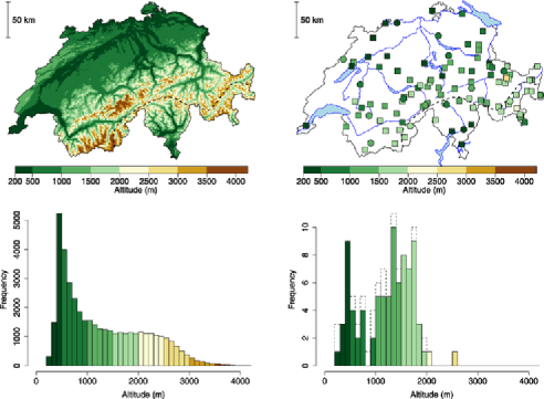
Figure 1: Topography and locations of stations for which daily snow depth data are available. First row: Topographical map of Switzerland (left) and station locations (right). Second row: Histogram of elevation of Switzerland at a $1$ km grid (left) and of the stations (right). Color indicates altitude in meters above mean sea level. Among the $101$ stations, $15$ (denoted by circles in the map on the right and by the dashed part of the right-hand histogram) are excluded from the analysis for validation. Dashed lines in the maps delimit the northern and southern slopes of the Alps.

2 Preliminaries

2.1 Data

We consider annual maximum snow depth from the $101$ stations whose locations are shown in Figure 1. The stations belong to two networks run by the WSL Institute for Snow and Avalanche Research (SLF) and the Swiss Federal Office for Meteorology and Climatology (MeteoSwiss). Annual maxima are extracted from daily snow depth measurements, which are read off a measuring stake at around 7.30 AM daily from November $1$st to April $30$th, for the 43 winters 1965–1966 to 2007–2008; we use the term “winter $1966$” for the months November $1965$ to April $1966$, and so forth. Examples of such time series can be found in the Supplementary Materials, Blanchet and Davison (2011). As Figure 1 shows, the stations are denser in the Alpine part of the country, which has high tourist infrastructure and increased population density and traffic during the winter months. Their elevations range from $250$ m to $2500$ m above mean sea level, with only two stations above $2000$ m. In order to validate our final model, we used $86$ stations to choose and fit the model and retained 15 stations for model validation.

2.2 Marginal analysis and transformation

Let $Z(x)$ denote the annual maximum snow depth at station $x$ of the set $\mathcal{X}$, which here denotes Switzerland. Data are only available at the stations $x\in\mathcal{D}\subset\mathcal{X}$, so modeling $Z(x)$ involves inference for the joint distribution of $\{Z(x),x\in\mathcal{X}\}$ based on observations from $\mathcal{D}$, and extrapolation to the whole of $\mathcal{X}$. In particular, as the station elevations lie mainly below $2000$ m, any results must be extrapolated to elevations higher than $2000$ m.

Daily snow depths at a given location $x$ are obviously temporally dependent. However, time series analysis suggests that, for every location $x\in\mathcal{D}$ and every winter, daily snow depths show only short-range dependence. Hence, distant maxima of daily snow depths seem to be near-independent and, therefore, the $D(u_{n})$ condition for independence of extremes that are well separated in time [Leadbetter et al. (1983), Section 3.2] should be satisfied. Extreme value theory is then expected to apply to annual maximum snow depth: $Z(x)$ at a location $x$ may be expected to follow a generalized extreme-value (GEV) distribution [Coles (2001)]

$$G(z)=\exp\biggl{[}-\biggl{\{}1+\xi(x)\frac{z-\mu(x)}{\sigma(x)}\biggr{\}}_{+}^{-1/\xi(x)}\biggr{]},$$ (1)

where $u_{+}=\max(u,0)$ and $\mu(x)$, $\sigma(x)>0$ and $\xi(x)$ are, respectively, location, scale and shape parameters.

Characterizing the probability distribution of $Z(x)$ for all $x\in\mathcal{X}$ is equivalent to characterizing the probability distribution of $f\{Z(x)\}$ for any bijective function $f$, which may be easier for a well-chosen $f$. A first step in our analysis is to transform the data at the stations to the unit Fréchet scale. Whatever the values of the GEV parameters $\mu(x)$, $\sigma(x)$ and $\xi(x)$, taking $f(z)=-1/\log G(z)$ transforms $\{Z(x),x\in\mathcal{X}\}$ into a spatial process $\{Z^{*}(x),x\in\mathcal{X}\}$ having unit Fréchet marginal distributions, $G^{*}(z)=\exp(-1/z)$. As it is easier to deal with $Z^{*}$ in general discussion, we will assume below that the time series at each station has been transformed in this way. To do so, one might model the GEV parameters $\mu(x)$, $\sigma(x)$ and $\xi(x)$ as smooth functions of covariates indexed by $x$, such as longitude, latitude and elevation [Padoan, Ribatet and Sisson (2010)]. However, due to the very rough topography of Switzerland and the influence of meteorological variables such as wind and temperature, snow depth exhibits strong local variation and additional covariates are necessary. A systematic discussion of such covariates and associated smoothing is given by Blanchet and Lehning (2010). The focus in the present paper is spatial dependence, so rather than adopt their approach, here we simply use GEV fits for the individual stations to transform $Z(x)$ at station $x\in\mathcal{D}$ into $Z^{*}(x)$. Diagnostic tools such as QQ-plots showed a good fit even at low altitudes.

2.3 Spatial dependence and regional patterns

A simple measure of the dependence of spatial maxima at two stations $x,x^{\prime}\in\mathcal{X}$ is the extremal coefficient $\theta_{xx^{\prime}}$. If $Z^{*}(x)$ is the limiting process of maxima with unit Fréchet margins, then [Coles (2001), Chapter 5]

$$\operatorname{pr}\{Z^{*}(x)\leq z,Z^{*}(x^{\prime})\leq z\}=\exp(-\theta_{xx^{\prime}}/z),\qquad z>0.$$ (2)

One interpretation of $\theta_{xx^{\prime}}$ appears on noting that

$$\operatorname{pr}\{Z^{*}(x^{\prime})>z|Z^{*}(x)>z\}\to 2-\theta_{xx^{\prime}},\qquad z\to\infty.$$

If $\theta_{xx^{\prime}}=1$, then the maxima at the two locations are perfectly dependent, whereas if $\theta_{xx^{\prime}}=2$, they are asymptotically independent as $z\to\infty$, so very rare events appear independently at the two locations. Although they do not fully characterize dependence, such coefficients are useful summaries of the multidimensional extremal distribution. In particular, it may be informative to compute all extremal coefficients $\{\theta_{xx^{\prime}},x^{\prime}\in\mathcal{X}\}$ for a given station $x$ to see how extremal dependence varies. Figure 2 depicts such maps for the snow depth data, for four different reference stations $x$. Extremal coefficients $\{\theta_{xx^{\prime}},x^{\prime}\in\mathcal{D}\}$ were estimated by the madogram-based estimator of Cooley, Naveau and Poncet (2006), and then kriged to the entire area using a linear trend on absolute altitude difference between $x$ and $x^{\prime}$. Similar maps have been proposed for gridded data by Coelho et al. (2008).

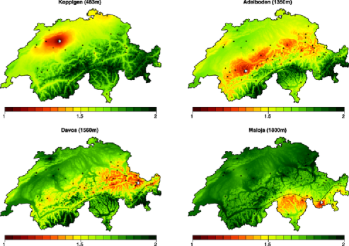
Figure 2: Extremal coefficient computed relative to Koppigen, Adelboden, Davos and Maloja (white points), estimated by the Cooley, Naveau and Poncet (2006) madogram estimator, and then kriged to the whole of Switzerland using a linear trend on absolute altitude difference.

Much information can be gleaned from Figure 2. A strong elevation effect is clearly visible. The map for Adelboden also suggests a directional effect: for this mid-altitude station in the Alps, there is more dependence with other middle-altitude stations in a roughly north-easterly direction. Another striking feature visible in the two lower maps is near-independence between the northern and southern slopes of the Alps. Further such maps suggest the presence of the two weakly dependent regions separated by the black dotted line in Figure 1. A similar north/south separation was seen in Blanchet, Marty and Lehning (2009), for good reason: extreme snowfall events occurring in these two regions typically do not stem from the same precipitation systems. Whereas extreme snowfall events on the northern slope of the Alps usually arise from northerly or westerly airflows [Schüepp (1978)], those in the southern slope usually come from the south or south-west. These are less frequent, but when they occur they can be very severe, due to the proximity of the Mediterranean Sea. As snow cover results from the accumulation of many snowfall events during the winter, one can expect annual maximum snow depths on the northern and southern slopes of the Alps to be somewhat disconnected. The winter of $1981$ illustrates this: little snow fell on the southern slope of the Alps, while the northern slope received large amounts. Figure 2 nevertheless suggests that these two regions are asymptotically weakly dependent, since $\theta_{xx^{\prime}}$ is generally larger than $1.7$, but not necessarily asymptotically independent. Even between well-separated stations, $\theta_{xx^{\prime}}$ is rarely very close to 2, perhaps owing to the rather small area under study, in which the largest distance between stations is around $350$ km.

3 Spatial maxima

3.1 Max-stable processes

The spatial dependence highlighted in Section 2.3 suggests that we model $Z^{*}(x)$ as a spatial process of extremes. A max-stable process with unit Fréchet margins is a stochastic process $\{Z^{*}(x),x\in\mathcal{X}\}$ with the property that, if $Z^{*}_{(1)}(x),\ldots,Z^{*}_{(n)}(x)$ are $n$ independent copies of the process, then [de Haan (1984)]

$$\Bigl{\{}\max_{i=1,\ldots,n}Z^{*}_{(i)}(x),x\in\mathcal{X}\Bigr{\}}\mbox{ has the same distribution as }\{nZ^{*}(x),x\in\mathcal{X}\}.$$

A consequence of this definition is that all finite-dimensional marginal distributions are max-stable: if $\{x_{1},\ldots,x_{D}\}$ is a finite subset of $\mathcal{X}$, then for all $n\in\mathbb{N}$,

$$\operatorname{pr}\{Z^{*}(x_{1})\leq nz_{1},\ldots,Z^{*}(x_{D})\leq nz_{D}\}^{n}$$

$$\qquad=\operatorname{pr}\{Z^{*}(x_{1})\leq z_{1},\ldots,Z^{*}(x_{D})\leq z_{D}\},\qquad z_{1},\ldots,z_{D}>0.$$

Such processes have several representations, two of which we now sketch.

3.2 Smith’s storm model

A general method of constructing max-stable processes is due to de Haan (1984). Let $\{(\eta_{i},s_{i}),i\in\mathbb{N}\}$ denote the points of a Poisson process on $(0,\infty)\times\mathcal{S}$ with intensity $\eta^{-2}d\eta\times\nu(ds)$, where $\mathcal{S}$ is an arbitrary measurable set and $\nu$ is a positive measure on $\mathcal{S}$. Let $\{f(s,x),s\in\mathcal{S},x\in\mathcal{X}\}$ denote a nonnegative function for which, for all $x\in\mathcal{X}$,

$$\int_{s\in\mathcal{S}}f(s,x)\nu(ds)=1.$$

Then the random process

$$Z^{*}=\Bigl{\{}\max_{i\in\mathbb{N}}\{\eta_{i}f(s_{i},x)\},x\in\mathcal{X}\Bigr{\}}$$ (3)

is max-stable with unit Fréchet margins. Smith (1990) gives a rainfall-storms interpretation of this construction. He suggests regarding $\mathcal{S}$ as a space of storm centers, of $f(s,\cdot)$ as the shape of a storm centered at $s$, and of $\eta$ as a storm magnitude. Then $\eta f(s,x)$ represents the amount of rainfall received at location $x$ for a storm of magnitude $\eta$ centered at $s$ and $Z^{*}(x)$ in (3) is the maximum rainfall received at $x$ over an infinite number of independent storms.

Additional assumptions are needed to get useful models from (3). Smith (1990) proposes taking $\mathcal{S}=\mathcal{X}=\mathbb{R}^{D}$, letting $\nu$ be the Lebesgue measure and $f(s,\cdot)$ be a multivariate normal density with mean $s$ and covariance matrix $\Sigma$, that is,

$$f(s,x)=(2\pi)^{-D/2}|\Sigma|^{-1/2}\exp\bigl{\{}-\tfrac{1}{2}(x-s)^{T}\Sigma^{-1}(x-s)\bigr{\}},\qquad x,s\in\mathbb{R}^{D}.$$

The resulting bivariate distribution of $Z^{*}$ defined by (3) at two stations $x_{1}$ and $x_{2}$ is then

$$\operatorname{pr}\{Z^{*}(x_{1})\leq z_{1},Z^{*}(x_{2})\leq z_{2}\}$$

(4)

$$\qquad=\exp\biggl{\{}-\frac{1}{z_{1}}\Phi\biggl{(}\frac{a}{2}+\frac{1}{a}\log\frac{z_{2}}{z_{1}}\biggr{)}-\frac{1}{z_{2}}\Phi\biggl{(}\frac{a}{2}+\frac{1}{a}\log\frac{z_{1}}{z_{2}}\biggr{)}\biggr{\}},$$

where $\Phi$ is the standard normal distribution function and $a$ is the Mahalanobis distance given by

$$a^{2}={(x_{1}-x_{2})^{T}\Sigma^{-1}(x_{1}-x_{2})}.$$ (5)

Below we will call this model the Smith process.

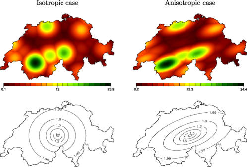
Figure 3: Smith’s process in two dimensions with two different matrices $\Sigma=(\tau_{dd^{\prime}})_{d,d^{\prime}\in\{1,2\}}$. Upper left image: a simulated field with $\tau_{11}=\tau_{22}=17^{2}$ and $\tau_{12}=0$ (isotropic case). Upper right image: a simulated field with $\tau_{11}=25^{2}$, $\tau_{22}=15^{2}$ and $\tau_{12}=14^{2}$ (anisotropic case). Lower images: corresponding pairwise extremal coefficient.

Two simulated Smith processes with different matrices $\Sigma$ are shown in the top row of Figure 3. The anisotropic case arises when $\Sigma$ is not spherical, that is, not of the form $\Sigma=\tau^{2}\mathbb{I}_{D}$, where $\tau^{2}>0$ and $\mathbb{I}_{D}$ is the identity matrix of side $D$. The resulting geometric anisotropy [e.g., Journel and Huijbregts (1978)] can easily be seen by computing pairwise extremal coefficients. Taking $z_{1}=z_{2}=z$ in (3.2) gives, according to (2),

$$\theta_{x_{1}x_{2}}=2\Phi(a/2).$$ (6)

The Mahalanobis distance $a$ appearing in (6) gives different weights to the different components of the vector $(x_{1}-x_{2})$. The limiting cases $a\rightarrow 0^{+}$ and $a\rightarrow+\infty$ correspond, respectively, to perfect dependence, $\theta_{x_{1}x_{2}}=1$, and independence, $\theta_{x_{1}x_{2}}=2$. For a given station $x_{1}$, surfaces $\{x_{2}\in\mathcal{X},\theta_{x_{1}x_{2}}=c\}$ are, according to (6), such that (5) is constant. If $\Sigma$ is spherical, then such surfaces are circles in two dimensions and spheres in three dimensions. Otherwise, they are ellipses and ellipsoids, respectively.

3.3 Schlather’s storm model

A second method of construction of max-stable processes was proposed by Schlather (2002). Let $\{\eta_{i},i\in\mathbb{N}\}$ denote the points of a Poisson process on $\mathbb{R}_{+}$ with intensity $\eta^{-2}d\eta$. Let $\{W(x),x\in\mathcal{X}\}$ be a stationary nonnegative process that satisfies $\mathbb{E}[W(x)]=1$ for all $x\in\mathcal{X}$, and let $W_{i}$, $i\in\mathbb{N}$, be independent copies of this process. Then [Schlather (2002)] the random process

$$Z^{*}=\Bigl{\{}\max_{i\in\mathbb{N}}\eta_{i}W_{i}(x),x\in\mathcal{X}\Bigr{\}}$$ (7)

is max-stable with unit Fréchet margins. When $W_{i}(x)=f(x-s_{i})$, where $f$ is a density function on $\mathcal{X}$ and the $s_{i}$ are the points of a Poisson process with unit rate on a measurable set $\mathcal{S}$, then (7) is equivalent to the storm model of Section 3.2. Smith’s model (3.2) corresponds to taking $f$ to be a multivariate normal density, extended by de Haan and Pereira (2006) to Student $t$ and Laplace densities. Like Smith’s model, the model (7) has a simple interpretation: the $\eta W$ are spatial events all having the same stochastic dependence structure but differing in their magnitudes $\eta$. An appealing difference between this and the Smith model is that the shapes of the events may vary if the process $W$ permits this.

Additional assumptions are again needed to get useful models from (7). Schlather (2002) proposes taking $W$ to be the positive part of a stationary Gaussian process with correlation function $\rho$, scaled so that $\mathbb{E}[\max\{0,\break W(x)\}]=1$ for all $x\in\mathcal{X}$. He shows that the corresponding bivariate distribution of $Z^{*}$ at two stations $x_{1}$ and $x_{2}$ is

$$\operatorname{pr}\{Z^{*}(x_{1})\leq z_{1},Z^{*}(x_{2})\leq z_{2}\}$$

(8)

$$\qquad=\exp\biggl{\{}-\frac{1}{2}\biggl{(}\frac{1}{z_{1}}+\frac{1}{z_{2}}\biggr{)}\biggl{(}1+\sqrt{1-2(\rho(h)+1)\frac{z_{1}z_{2}}{(z_{1}+z_{2})^{2}}}\biggr{)}\biggr{\}},$$

where $h\in\mathbb{R}_{+}$ is the Euclidean distance $\|x_{2}-x_{1}\|$ between the two stations. Below we call this max-stable model Schlather’s process.

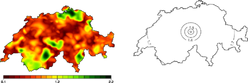
Figure 4: Schlather’s process in two dimensions for a Cauchy covariance function $\rho(h)=(1+h^{2}/19^{2})^{-1}$. Left image: one simulated field. Right image: corresponding pairwise extremal coefficient.

A simulation from an isotropic version of this model with $\mathcal{X}$ corresponding to Switzerland is shown in Figure 4. The isotropy can be easily seen by computing pairwise extremal coefficients. Taking $z_{1}=z_{2}=z$ in (3.3) gives, according to (2),

$$\theta_{x_{1}x_{2}}=1+\biggl{\{}\frac{1-\rho(\|x_{1}-x_{2}\|)}{2}\biggr{\}}^{1/2}.$$ (9)

Here the extremal coefficients involve the Euclidean distance between the two locations. For a given station $x_{1}$, surfaces with the same extremal coefficents $c\in[1,2]$, that is, surfaces $\{x_{2}\in\mathcal{X},\theta_{x_{1}x_{2}}=c\}$, are, according to (9), such that $\|x_{1}-x_{2}\|=c^{\prime}$. Such surfaces are circles in two dimensions and spheres in three dimensions. The limiting case $\|x_{1}-x_{2}\|\rightarrow 0^{+}$ corresponds to perfect dependence, $\theta_{x_{1}x_{2}}=1$. If, like most geostatistical correlation functions, the underlying Gaussian process has $\rho(h)\rightarrow 0$ when $h\rightarrow+\infty$, then the limiting case $\|x_{1}-x_{2}\|\rightarrow+\infty$ corresponds to $\theta_{x_{1}x_{2}}=1+2^{-1/2}\approx 1.707$, and so independent extremes do not arise even at very large distances. Moreover, as an isotropic correlation function can give correlations no smaller than $-0.403$ in $\mathbb{R}^{2}$ and $-0.218$ in $\mathbb{R}^{3}$ [Matérn (1986), page 16], under Schlather’s model we have $\theta_{x_{1}x_{2}}\leq 1.838$ for any $x_{1}$, $x_{2}$ in $\mathbb{R}^{2}$ and $\theta_{x_{1}x_{2}}\leq 1.780$ for any $x_{1}$, $x_{2}$ in $\mathbb{R}^{3}$. Thus, it is impossible to produce independent extremes using such a process, no matter how distant the stations. Davison and Gholamrezaee (2010) have proposed extensions to allow independence in (3.3), and Kabluchko, Schlather and de Haan (2009) have extended both Smith’s and Schlather’s representations.

4 Max-stable process for extreme snow depth

4.1 General

As pointed out in Section 2.3, snow depth data show two key characteristics that should be explicitly modeled in the max-stable process. First, dependence is anisotropic, due to the strong elevation effect and the presence of a main direction of dependence. Second, Switzerland seems to be divided into two weakly dependent climatic regions: the northern slope of the Alps together with the Plateau, which is the low altitude region north of the Swiss Alps; and the southern slope of the Alps. In this section we propose to extend the Smith and Schlather models of Sections 3.2–3.3 to account for these features. Other representations described in Kabluchko, Schlather and de Haan (2009), in Davison and Gholamrezaee (2010) or in Davison, Padoan and Ribatet (2010) are not considered in this paper.

4.2 Modeling anisotropy

Smith’s model can directly model anisotropy using a nonspherical $\Sigma$ matrix in (3.2). The simple version of Schlather’s model is isotropic, but it can easily account for anisotropy by considering a transformed space $\mathcal{\tilde{X}}$ instead of $\mathcal{X}$.

Anisotropy of Smith’s model arises from the fact that the distance used in the extremal coefficient (6) is Mahalanobis distance (5) rather than Euclidean distance. Using the eigendecomposition $\Sigma=U\Lambda U^{T}$, where $U$ is a rotation matrix and $\Lambda$ a diagonal matrix of positive eigenvalues, we may write

$$\Sigma^{-1}=U^{T}\Lambda^{-1}U=(\Lambda^{-1/2}U)^{T}(\Lambda^{-1/2}U),$$ (10)

where $\Lambda^{-1/2}$ denotes the diagonal matrix composed of the reciprocal square roots of the diagonal elements of $\Lambda$. If $\lambda_{1}$ denotes the first element of $\Lambda$, then (10) can be written as $\Sigma^{-1}=\lambda_{1}^{-1}V^{T}V$, where $V=\lambda_{1}^{1/2}\Lambda^{-1/2}U$. The squared Mahalanobis distance (5) is

$$a^{2}=\frac{1}{\lambda_{1}}(x_{1}-x_{2})^{T}V^{T}V(x_{1}-x_{2})=\frac{1}{\lambda_{1}}[V(x_{1}-x_{2})]^{T}[V(x_{1}-x_{2})],$$

which is exactly that between $\tilde{x}_{1}=Vx_{1}$ and $\tilde{x}_{2}=Vx_{2}$ in the isotropic case, that is, when using a $D$-dimensional spherical covariance matrix $\lambda_{1}\mathbb{I}_{D}$ in (3.2). Thus, the anisotropic Smith model on $\mathcal{X}$ is just the isotropic Smith model on the transformed space $\mathcal{\tilde{X}}=V\mathcal{X}$.

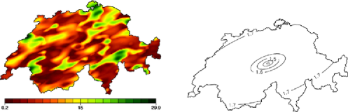
Figure 5: Anisotropic Schlather model resulting from climate space transformation. Left image: a simulated field. Right image: corresponding extremal coefficients.

Similar ideas can be used with Schlather’s model, by applying it on $\mathcal{\tilde{X}}=V\mathcal{X}$, where in three dimensions we may take

$$V=\pmatrix{\cos\alpha&-\sin\alpha&0\cr c_{2}\sin\alpha&c_{2}\cos\alpha&0\cr 0&0&c_{3}},\qquad c_{2},c_{3}\in\mathbb{R}_{+}^{*},$$ (11)

as for Smith’s model. In the rest of the paper we will use the term climate space for the transformed space $\mathcal{\tilde{X}}=V\mathcal{X}$ in which isotropy is achieved. Figure 5 illustrates the climate space transformation, allowing an anisotropic Schlather model, with the same $V$ matrix as that corresponding to the anisotropic case of Figure 3. Compared to Figure 4, constant extremal coefficients correspond to ellipses, allowing us to model directional effects.

Geometric anisotropy as induced by the $V$ matrix is a special case of range anisotropy [Zimmerman (1993)]. In the nonextremal framework, this idea has been extended to nongeometric range anisotropic models, in which nested covariances are used with different range parameters in different directions, but in general this does not define a valid covariance function. Ecker and Gelfand (2003) introduced product geometric anisotropy, under which covariance functions are products of geometric anisotropic covariances. Space transformation has also been used by Sampson and Guttorp (1992) to model nonstationary spatial covariance structures, allowing more complex transformations than the affine transformation considered here. In addition to these global methods, local methods for modeling anisotropy and more general forms of nonstationarity also exist. These can be divided in three main families [Schabenberger and Gotway (2005)]. The moving window approach of Haas (1990) estimates a covariance function locally within a neighborhood. The convolution method of Higdon (1998) allows the construction of weakly nonstationary processes by convolving a zero-mean white noise process with a kernel function whose parameters can depend on location. The method of weighted stationary processes [Fuentes (2001)] allows one to write the nonstationary covariance function as a weighted mixture of isotropic covariances, where the weights depend on the location. Fuentes, Henry and Reich (2010) use a Dirichlet process mixture as the basis for a flexible copula approach to space-time modeling of extreme temperatures, but it does not correspond to a max-stable process model, and the relatively long-range dependence of temperatures can be modeled more simply than can precipitation phenomena such as rain- and snowfall. It would be very valuable to apply these ideas in the max-stable context, but the unavailability of a likelihood function seems to be a major obstacle.

The idea of space transformation was used by Cooley, Nychka and Naveau (2007) in modeling US precipitation. Instead of using the three-dimensional geographical coordinates (longitude, latitude, elevation) for locating stations, the authors work in a “climate space,” namely, the two-dimensional space given by elevation and mean precipitation for the months April to October. Unlike in Cooley, Nychka and Naveau (2007), our transformation is affine, giving more weight to elevation through $c_{3}$, and defining a main direction of dependence along the $\alpha$-axis. A higher-dimensional space could of course be used for $\mathcal{X}$. In particular, one could use the four-dimensional space of (longitude, latitude, elevation, mean snow depth), thus blending the Cooley, Nychka and Naveau (2007) approach with ours; see Section 6.

4.3 Modeling climate regions

Different approaches to accounting for the impact of the climate regions on the extremes are possible:

1. The climate regions are independent. This is equivalent to saying that two max-stable processes govern the two regions independently. In terms of spatial dependence, extremal coefficient maps will be of the form of Figure 3 or 5 but replacing the Swiss border by the border of the northern region alone for the pairwise dependence with a station located in the north, and similarly for the southern region.

2. The climate regions are weakly dependent. Since dependence between pair of stations decreases when distance increases, one way to model weakly dependent regions is to increase the distance between them. This can be done by adding to $\mathcal{X}$ a coordinate equal to $0$ in the northern region, and to $1$ in the southern region. If the other coordinates are (longitude, latitude, elevation), then the $V$ matrix of the climate space transformation (11) can be written in the most general case as a $4\times 4$ matrix with one column comprising $0$ apart from one element. Nevertheless, for computational reasons it may be better to consider the rotation matrix $U$ of Section 4.2 as being a rotation matrix in the (longitude, latitude) plane and thus to set

   $$V=\pmatrix{\cos\alpha&-\sin\alpha&0&0\cr c_{2}\sin\alpha&c_{2}\cos\alpha&0&0\cr 0&0&c_{3}&0\cr 0&0&0&c_{4}};\vspace*{3pt}$$ (12)

   we shall do this in Section 6. In the four-dimensional climate space $\mathcal{\tilde{X}}=V\mathcal{X}$, the squared distance between two stations $x_{1}$ and $x_{2}$ is $\{V(x_{1}-x_{2})\}^{T}\{V(x_{1}-x_{2})\}$. But the fourth coordinate of $x_{1}-x_{2}$ is $0$ if the two stations belong to the same region and $\pm 1$ otherwise. The squared distance will then equal that in the (longitude, latitude, elevation) climate space if the two stations are in the same region, and be increased by $c_{4}^{2}$ otherwise. We thus increase the distance between the climate regions, and therefore decrease the dependence between them, without increasing the distance between stations of the same region. To see how the extremal coefficients behave, see the left-hand side of Figure 6.

3. The climate regions are weakly dependent in continuous space. Since the additional coordinate introduced above jumps from $0$ to $1$ at the border between the regions, it induces a discontinuity of the extremal coefficients which is visible in the left map of Figure 6; see the cyan and magenta ellipses. This seems unrealistic and something smoother is preferable. An easy way to impose space continuity is to take the border to be a band inside which the fourth coordinate is linearly interpolated between $0$ and $1$, with value $0$ on the upper-border of the band and $1$ on the lower-border. With this simple interpolation, there is no jump at the border and curves of constant extremal coefficient are continuous, as in the right-hand side of Figure 6. The width of the band must be estimated from the data; we return to this in Section 5.

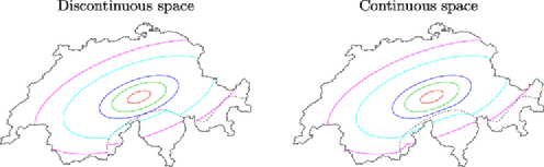
Figure 6: Example of extremal coefficients with weakly dependent regions in discontinuous space (left image) and continuous space (right image). The images are the same, except in a 10 km wide band around the north/south border (dashed line).

5 Model estimation and selection

5.1 Pairwise likelihood

Statistical inference for parametric models is ideally performed using the likelihood function. Let $\mathcal{D}=\{x_{1},\ldots,x_{D}\}\subset\mathcal{X}$ denote the $86$ stations whose maxima are used for fitting the models. Computation of the likelihood requires the joint density function of $\{Z^{*}(x_{1}),\ldots,Z^{*}(x_{D})\}$, but in the framework of max-stable processes, this is infeasible because only the bivariate marginal distributions are available. Padoan, Ribatet and Sisson (2010) proposed replacing the full likelihood by a pairwise likelihood function [Cox and Reid (2004); Varin (2008)]. This idea is also used by Davison and Gholamrezaee (2010), Davison, Padoan and Ribatet (2010) and by Smith and Stephenson (2009), the latter in a Bayesian framework.

Let $z_{ik}$ denote the $k$th observed maximum for the $i$th station, transformed so that time-series $(z_{i1},\ldots,z_{iK})$ at each station have unit Fréchet distributions; here $k\in\{1,\ldots,K\}$, with $K=43$ years, and $i\in\{1,\ldots,D\}$, with $D=86$ stations. Let ${\beta}=(\beta_{1},\ldots,\beta_{R})$ denote the parameters to be estimated. Then the pairwise marginal log-likelihood is

$$\ell_{\mathrm{p}}({\beta})=\sum_{k=1}^{K}\sum_{i<j}\log f(z_{ik},z_{jk};{\beta}),$$ (13)

where $f(\cdot,\cdot)$ is the bivariate density of the unit Fréchet max-stable process, that is, the derivative of equation (3.2) for Smith’s model or of (3.3) for Schlather’s model, and the second summation is over all distinct pairs of stations, $D(D-1)/2$ terms in all. Under suitable regularity conditions, the maximum pairwise maximum likelihood estimator $\check{\beta}$ has a limiting normal distribution as $K\rightarrow+\infty$, with mean ${\beta}$ and covariance matrix of sandwich form estimable by $H({\check{\beta}})^{-1}J({\check{\beta}})H({\check{\beta}})^{-1}$, where

$$H({\beta}) = -\sum_{k=1}^{K}\sum_{i<j}\frac{\partial^{2}\log f(z_{ik},z_{jk};{\beta})}{\partial{\beta}\partial{\beta}^{T}},$$ (14)

$$J({\beta}) = \sum_{k=1}^{K}\sum_{i<j}\frac{\partial\log f(z_{ik},z_{jk};{\beta})}{\partial{\beta}}\frac{\partial\log f(z_{ik},z_{jk};{\beta})}{\partial{\beta}^{T}}$$ (15)

are the observed information matrix and the squared score statistic corresponding to $\ell_{\mathrm{p}}$. The use of the pairwise likelihood estimator for Smith’s process was validated by Padoan, Ribatet and Sisson (2010) in a simulation study.

5.2 Estimation in practice

Estimating the maximum pairwise likelihood estimator requires the maximization of (13) with respect to the $R$ parameters. We found that the R function optim gave quite poor results for our application: the surface $\ell_{\mathrm{p}}$ can have many local maxima, and optim and similar functions find it hard to deal with them. After some experimentation, we therefore adopted a profile likelihood method. Given a set of $(R-1)$ parameters ${\beta}_{-r}$, it is easy to find the value of $\beta_{r}$ that maximizes the single-variable function $\ell_{\mathrm{p}}(\cdot,{\beta}_{-r})$. This suggests the following iterative algorithm:

1. Take initial parameters ${\beta}=(\beta_{1},\ldots,\beta_{R})$.

2. For $r$ in $1,\ldots,R$:

   1. [(a)]

   2. find the value $\check{\beta}_{r}$ that maximizes the pairwise likelihood with respect to the scalar $\beta_{r}$, holding the other parameters, ${\beta}_{-r}$, fixed, that is,

      $$\check{\beta}_{r}=\arg\max_{\beta_{r}}\ell_{\mathrm{p}}(\beta_{r},{\beta}_{-r});$$

   3. then update the $r$th component of ${\beta}$ to $\check{\beta}_{r}$.

3. Go to step 2, stopping when no change to any $\beta_{r}$ can increase the pairwise log-likelihood.

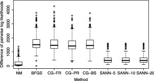
Figure 7: Difference in pairwise log-likelihood at convergence between the profiling algorithm and eight algorithms for simultaneous parameter estimation, for 200 simulated data sets. The eight algorithms are: Nelder–Mead, NM; the quasi-Newton method of Broyden, Fletcher, Goldfarb and Shanno, BFGS; three conjugate gradient methods, CG-FR, CG-PR and CG-BS; and a variant of simulated annealing using starting temperatures of 5, 10 and 20, SANN-5, SANN-10 and SANN-20. The help for the R function optim gives more details of these algorithms.

To assess the performance of this algorithm, we simulated 200 data sets, each comprising $43$ independent copies of Schlather’s max-stable random field (3.3) with Cauchy covariance function $\rho$ in a three-dimensional climate space. Each of the copies is observed at the same $D=100$ stations, so the number of observations is very similar to those for the annual snow depth data; see Section 2.1. The climate transformation is defined through a $3\times 3$ matrix $V$ as in (11). The model has three parameters for the $V$ matrix and two for the covariance function, which induces middling dependence: about 25% of the pairs of stations have extremal coefficients $\theta\leq 1.68$; recall from Section 3.3 that for Schlather’s model, $\theta\leq 1.707$. We started from the same initial point for each of the $200$ data sets and optimized the log pairwise likelihood (13) with (i) eight optimization procedures within the R function optim with all parameters estimated jointly [Blanchet and Davison (2011)]; and (ii) the above profile likelihood algorithm. Figure 7 shows the differences between the pairwise log-likelihoods for the methods at convergence, for the 200 data sets. The profiling method never gives lower maximized pairwise likelihoods than the other algorithms, and they are almost always higher. Further simulations with small- and large-range dependence gave similar results [Blanchet and Davison (2011)]: overall profiling is clearly better than the other algorithms. Those that compare best with profiling, viz., Nelder–Mead and simulated annealing, are designed for rather rough surfaces with many local optima. These simulated data are relatively simple compared to the real data, which are neither exactly unit Fréchet after transformation from (1) nor follow a pure max-stable process. Furthermore, the max-stable model used for the simulation is quite simple, with only five parameters to be estimated, so the profiling approach seems necessary for our, more complex, application.

5.3 Model selection

Model selection criteria play an important role in deciding which of the fitted models should be preferred. As in Padoan, Ribatet and Sisson (2010), we propose to use the composite likelihood information criterion [Varin and Vidoni (2005)], which extends the $\mathrm{TIC}$ [Takeuchi (1976)] to the composite likelihood setting, and is defined as

$$\mathrm{CLIC}=-2\ell_{\mathrm{p}}(\check{{\beta}})+2\operatorname{tr}\{H(\check{{\beta}})^{-1}J(\check{{\beta}})\},$$

where $H$ and $J$ are, respectively, the observed information matrix and the squared score statistic corresponding to $\ell_{\mathrm{p}}$, defined at equations (14) and (15), and $\check{{\beta}}$ is the maximum pairwise likelihood estimator. Lower values of $\mathrm{CLIC}$ correspond to better quality models.

6 Application to snow depth in Switzerland

6.1 Fitted models

We fitted the different models described in Section 4 to our snow depth data, using both Smith and Schlather max-stable structures for the extremes. For Schlather’s model, different choices of Gaussian covariance function $\rho$ lead to different distributions (3.3). We used nine such functions, namely, the spherical, circular, cubic, Gneiting, exponential, Matérn, Gaussian, powered-exponential and Cauchy covariance functions [Banerjee, Carlin and Gelfand (2003); Schabenberger and Gotway (2005)]. Each has either one or two parameters and the first four have an upper bound. They all are such that $\rho(h)\rightarrow 1$ when $h\rightarrow 0^{+}$ and $\rho(h)\rightarrow 0$ when $h\rightarrow+\infty$. As mentioned in Section 3.3, this constrains the extremal coefficient for Schlather’s model to correspond to dependent data. Nevertheless, we will see that such an assumption seems justified in our case.

The coordinates $x$ we considered are geographical coordinates (longitude, latitude, elevation), region number (see Section 4.3) and mean snow depth during the winters 1966–2008. Mean precipitation was considered as a possible climate coordinate in Cooley, Nychka and Naveau (2007)’s study of extreme precipitation. The idea of using mean snow depth is that stations with similar snow depth are probably influenced by the same weather patterns and should therefore be closer in the climate space than are stations with different snow cover. Other climate variables that could be considered are temperature, wind direction and wind speed, which are also measured at the stations, but these values are of relatively poor quality with many missing values, so we decided not to use them.

In addition to the models illustrated in Section 4, we allowed the possibility of having different climate spaces in northern and southern regions, that is, to have different climate space transformation matrices $V$. In three dimensions, for example, two $V$ matrices as in (11) will have to be estimated, with a total of 6 parameters. In the continuous-space case illustrated in Figure 6, all coefficients $\alpha$ and $c$ are linearly interpolated around the north/south border. We also considered different mixtures of the above possible coordinates. In all cases, we used longitude and latitude, plus possibly the elevation, region number and mean snow depth, or combinations of these three coordinates. In total, $65$ types of models were considered, each of them being estimated for one Smith and nine Schlather processes, giving $650$ fits in all. A description of the 65 model types is given in the Supplementary Materials [Blanchet and Davison (2011)]. All were estimated using the iterative profiling algorithm of Section 5.2.

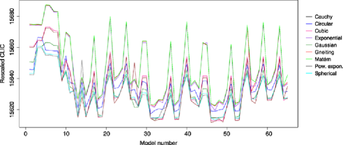
Figure 8: Rescaled $\mathrm{CLIC}$ values for all $65\times 9$ fitted Schlather models.

6.2 Model comparison

A summary of the $\mathrm{CLIC}$ values for the 585 fitted Schlather models, rescaled by division by $D-1$ in order to give log-likelihood values that would correspond to independent data, is shown in Figure 8. There are relatively small differences among them, though the Gneiting and Gaussian covariance functions seem to perform less well and the spherical and circular covariance functions have the $25$ best $\mathrm{CLIC}$ values. These covariance functions have an upper bound and are governed by only one parameter. Schlather’s model always performs better than Smith’s model, whatever the chosen covariance function: the rescaled $\mathrm{CLIC}$ with Smith’s model is between 30 and 300 units higher than with Schlather’s model, with a minimum value of 15,650 attained for model 47. Whether with Smith or Schlather models, the same patterns appear. In particular, the first eight models, which perform poorly, correspond to models in Euclidean space, without climate space transformation. The benefit of working in a transformed space in order to allow for anisotropy is thus clear. This effect is particularly striking for Smith’s model, for which it is equivalent to saying that a nonspherical $\Sigma$ matrix (see Section 3.2) should be used: there is a difference of 300 between the lowest rescaled $\mathrm{CLIC}$ values in the Euclidean and climate spaces. The models numbered $10$, $11$, $17$, $21$, $25$, $29$, $30$, $36$, $40$, $44$, $45$, $51$, $55$, $59$ and $63$, which are also poor, correspond to cases when neither elevation nor the mean snow depth are considered [Blanchet and Davison (2011)]. As the mean snow depth is strongly related to elevation, the latter is a very important climate coordinate. It seems to be more informative than the mean snow depth; models using elevation but not mean snow depth as a coordinate always have lower $\mathrm{CLIC}$ values than in the converse case.

Table 1: Parameters (standard errors) of the model selected by $\mathrm{CLIC}$: Schlather’s model with spherical covariance function, two climate transformations but a continuous space (the band around the north/south border is about $5$ km wide)

Covariance parameter
$447.45\ (43.32)$
	Climate space parameters
	Main direction	Latitude (km)	Elevation (km)	Mean snow	Region num.
	(radian)			depth (cm)
North	$0.36\ (0.03)$	$4.98\ (0.80)$	$274.7\ (35.4)\hphantom{0}$	$1.26\ (0.46)$	$\times$
South	$0.17\ (0.06)$	$4.70\ (1.16)$	$406.5\ (161.3)$	$6.41\ (2.45)$	$449.4\ (37.4)$

6.3 Selected model

According to the $\mathrm{CLIC}$, the best fit is given by Schlather’s model with spherical covariance function, and a 5-dimensional climate space $\mathcal{X}$ of coordinates (longitude, latitude, elevation, region number, mean snow depth) with different transformations in the north and south but imposing space continuity; this, model number 47 in Blanchet and Davison (2011) has a $\mathrm{CLIC}=15\mbox{,}611.66$. This means that two $V$ matrices are estimated, each of the form (12) but in five dimensions, and thus having five parameters: the main direction of dependence, and the four parameters $c$ associated to the latitude, elevation, region number and mean snow depth. Since the region number is a binary variable, the $c$ value for the northern region can be fixed equal to zero. The range parameter of the spherical covariance function and the width of the band between the regions are also estimated, for a total of $11$ parameters, whose estimates and standard errors are shown in Table 1. As the pairwise likelihood is not differentiable with respect to the band width, no standard error is given for it. The second- and third-best fits are also obtained with spherical covariance functions with similar models as in Table 1 but without the mean coordinate (model number 49, with $\mathrm{CLIC}=15\mbox{,}612.03$) or the region number coordinate (model number 46, with $\mathrm{CLIC}=15\mbox{,}612.56$), that is, using a four-dimensional space $\mathcal{X}$. In the latter case, values of the estimated coefficients are such that the northern and southern regions are disjoint in the climate space, although no region number coordinate is used to separate them. These two models perform similarly because the mean coordinate should provide information about the local variability of snow depth, part of which agrees with the regional division between the northern and southern slopes; thus, the mean coordinate and region number carry similar information. According to Figure 8, it seems better to use both coordinates, but using one of them increases the $\mathrm{CLIC}$ only very slightly.

It is no surprise that in Table 1, elevation is the most influential coordinate in the climate distance, and thus in the dependence function. In the north, for example, dependence between two stations at the same elevation but $10$ km apart along the main direction of dependence, an angle of $\alpha=0.36$ radians in the sense of an Argand diagram, at the same elevation but $2$ km apart perpendicularly to the main direction of dependence, and at the same latitude and longitude but $40$ m apart in elevation, are all equal. An interesting feature is the main direction of dependence in the northern region, which can be explained by two facts:

1. due to the strong elevation effect, the north slope of the Alps (the mountainous part of the northern region) is very weakly dependent on the Plateau (the low-elevation part of the northern region). But both subregions are oriented along the North Alpine ridge, and dependence is thus higher in this direction;

2. this direction is also broadly that of the two widest valleys in Switzerland, the Rhone and Rhine valleys, as shown by the main green valleys in Figure 1. These are wide enough to direct snow-bearing clouds along them, thus inducing strong directional dependence of precipitation.

The high value associated to the region number coordinate gives the lowest possible dependence, $\theta_{xx^{\prime}}=1.707$, between extremes in the northern and southern regions.

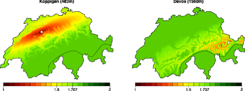
Figure 9: Pairwise extremal coefficient with Koppigen and Davos (white circles) predicted by the selected max-stable model.

Figure 9 shows maps of the estimated pairwise dependence under the max-stable model of Table 1, obtained by extrapolating the mean snow depth at ungauged stations where no data are available. To do this, we performed spatial kriging with a spline dependence on elevation, to allow for the fact that temperatures at stations below $800$ m may exceed $0^{\circ}$C even when it is snowing at higher altitudes, leading them to suffer rain rather than snow. The resulting smooth mean process was successfully validated on the additional $15$ stations [Blanchet and Davison (2011)]. Figure 9 clearly shows both the elevation effect and the weak north/south dependence. The low bandwidth, of about $5$ km, induces an abrupt change of the extremal coefficient around the north/south border.

6.4 Model checking

For a first check on the quality of the selected model, we compare its predicted extremal coefficients, obtained by replacing the parameters involved in (9) by their estimates from Table 1, with the naive estimators of Schlather and Tawn (2003) or the madogram-based estimator of Cooley, Naveau and Poncet (2006). As the extremal coefficients (9) are functions of distance between stations, we plot naive and predicted extremal coefficients against distance. Figure 10 shows such comparisons for our selected model and for the best Smith model. For clarity, we only show the madogram-based estimator of Cooley, Naveau and Poncet (2006), with and without binning. The naive estimators of Schlather and Tawn (2003) give essentially the same picture, but with slightly higher variability.

Figure 10 shows that the Smith model fits the data less well than the Schlather model. In particular, the extremal coefficient curve of the Smith model crosses the point cloud for the binned madogram, whereas our selected model follows it quite well up to a climate distance of $400$, and then underestimates it. A limit of about $1.8$ would be expected from the madogram, but cannot be attained with Schlather’s model; see Section 7.

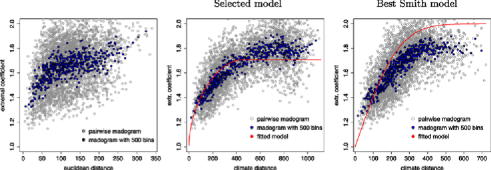
Figure 10: Extremal coefficient for pairs of stations as a function of the distance between them, in Euclidean space (left plot) or climate space (center and right). The red curve is the extremal coefficient curve for the corresponding max-stable model.

Another way to check our model is to compare the empirical distribution of maxima of subsets of stations, that is, $Z^{*}_{\mathcal{A}}=\max\{Z^{*}(x_{i}),x_{i}\in\mathcal{A}\}$, with maxima predicted by the selected model. The distribution of $Z^{*}_{\mathcal{A}}$ under the selected model is known analytically only when $\mathcal{A}$ comprises two stations, but samples of $Z^{*}_{\mathcal{A}}$ can be simulated for any $\mathcal{A}$. Since realizations $z^{*}_{\mathcal{A}}$ of $Z^{*}_{\mathcal{A}}$ are available for $K=43$ years, one can compare the empirical quantiles of $Z^{*}_{\mathcal{A}}$ with the simulated ones. More precisely, given a subset $\mathcal{A}$, we simulate $M$ independent series ${z^{*(m)}_{\mathcal{A}}}$ of length $K$, and thus obtain $M$ replicates of the observed Fréchet series $z^{*}_{\mathcal{A}}$. Ordered values of observed $z^{*}_{\mathcal{A}}$ can then be compared with ordered values of the ${z^{*(m)}_{\mathcal{A}}}$ as a graphical test of fit. Pointwise and overall confidence bands can also be derived from these simulations [Davison and Hinkley (1997), Section 4.2.4].

Figure 11 uses this approach to compare fitted and empirical distributions for different groups of three or four stations taken from the 15 not used to fit the model, some groups being tightly clustered, and others being dispersed. The fit seems to be broadly satisfactory in all cases. Even the dependence between stations whose climate distance is larger than $500$ units seems to be well-modeled, despite the mismatch between the fitted and empirical pairwise extremal coefficients at such distances seen in Figure 10.

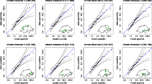
Figure 11: Comparison of empirical and model quantiles for annual maxima of groups of stations not used in the fitting. The stations used for each panel are shown in its map, and the envelopes are 95% pointwise and overall confidence bands obtained from $M=5\mbox{,}000$ simulations.

6.5 Risk analysis

For risk management it is important to be able to assess how extreme events are likely to occur in the same year in different places. A first answer to this question can be obtained by computing probabilities of the form $\operatorname{pr}[\{Z^{*}(x)>z,x\in\mathcal{A}\}]$ for a group of stations $\mathcal{A}$ and different high levels $z$. Figure 12 plots such probabilities for different groups $\mathcal{A}$ when $z$ is the $r$-year return level of the unit Fréchet distribution. By back-transformation from equation (1), this is equivalent to computing the joint survival distributions $\operatorname{pr}[\{Z(x)>\mathrm{RL}_{r}(x),x\in\mathcal{A}\}]$ where $\mathrm{RL}_{r}(x)$ denotes the $r$-year return level at station $x$, that is, the probability that all stations in $\mathcal{A}$ receive more snow a given year than their $r$-year return level. Under independence, this probability equals $r^{-|\mathcal{A}|}$ for any possible set $\mathcal{A}$, where $|\mathcal{A}|$ is the number of stations in $\mathcal{A}$, whereas it equals $r^{-1}$ under full dependence. Figure 12 shows very good agreement between the observed and predicted distributions using the model, whereas the risk is underestimated under the hypothesis of independent stations and overestimated under the hypothesis of full dependence. The underestimation is more striking for quite dependent stations, such as those in the left-hand panel of Figure 12. When distance increases, the difference between the dependent and independent cases is less striking but our max-stable model fits better even for pairs of stations that are $980$ climate distance units apart; this is almost the largest climate distance between pairs of stations. The right-hand panel corresponds to a group of seven stations in the eastern Plateau. Our model clearly gives more realistic risk probabilities than does the independence assumption. Extreme snow events in the low-elevation Plateau generally occur over a large region due to the easy weather circulation. A typical example is the extraordinary snowfall event that occurred on March 5th 2006 over the entire Plateau, with snow measurements of $54$ cm at Zurich, $49$ cm at Basel and $60$ cm at Sankt Gallen. This was the largest snow depth recorded since 1931 [Zanini, Sutter and Gerstgrasser (2006)].

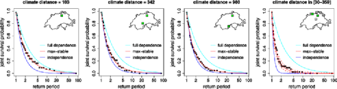
Figure 12: Risk analysis of groupwise annual maxima: joint survival probability versus return period. In the right-hand of each panel the envelope is a 95% pointwise confidence band obtained from $M=5\mbox{,}000$ simulations. Stations indicated in green were not used for fitting.

7 Discussion

The models discussed here are a step toward modeling spatial dependence of extreme snow depth. They are based on the Smith (1990) and Schlather (2002) max-stable representations, designed to model extreme snow depth explicitly. In particular, they can account in a flexible way for the presence of weakly dependent regions. They involve a climate transformation that enables the modeling of directional effects resulting from phenomena such as weather system movements. In the proposed methodology, model fitting is performed by using a profile-like method for maximizing the pairwise likelihood function, and model selection is performed using an information criterion.

We applied this methodology to $86$ stations with recorded snow depth maxima. Performance of the selected model at small and large scales was assessed on these stations, together with $15$ other stations, by comparing empirical and predicted distributions of group of stations. By accounting for spatial dependence, our model gives clearly more realistic probabilities of extreme co-occurrence than would a nonspatial model. Such quantities are important for adequate risk management.

Considered as a whole, the max-stable models proposed in this paper constitute a family of flexible models that could potentially be applied to other kinds of climate data, in particular, extreme precipitation and temperature. Further improvements could nevertheless be investigated, as discussed below.

In this paper we focus on modeling the spatial dependence of extremes, rather than on the marginal distributions. A first step was thus to transform maxima from their original scale to a common unit Fréchet distribution. In the application to snow depth data, this transformation was done by using the GEV distributions fitted to the time series, considered separately. A fuller spatial model would consider the three GEV marginal parameters as response surfaces. Using the models presented in this paper, one could then simultaneously estimate the spatial dependence and the spatial intensity of maxima, following Padoan, Ribatet and Sisson (2010) and Davison and Gholamrezaee (2010). These authors use simple functions of longitude, latitude and elevation, but the very complex Alpine topography results in an extremely variable pattern of snow, and we were unable to find satisfactory marginal response surfaces for our application. Blanchet and Lehning (2010) describe other approaches that appear to be more satisfactory, but modeling of the margins requires more investigation. Time could be used as a covariate in order to allow for the potential impact of climate change on extreme snow events; for example, the retreat of the glaciers is strongly affecting microclimates at high altitudes. This notwithstanding, exploratory work suggests that although climate change has affected mean snow levels [Marty (2008)], its effect on extreme snow events is not yet discernible, except possibly at low elevation [Laternser and Schneebeli (2003)].

A second improvement might be the consideration of event times, which could be incorporated into the pairwise maximum likelihood procedure [Stephenson and Tawn, (2005)]. For our data, the co-occurrence of annual maxima is quite variable. For winters such as those of 1975 and 2006, snow depth reached its maximum almost simultaneously all over Switzerland. For winters such as those of 1980, 2007 and 2008, the annual maxima occurred at quite different dates; see the Supplementary Materials, Blanchet and Davison (2011). Including this information by modifying the pairwise likelihood contribution of maxima occurring simultaneously at two stations might yield more precise inferences, as shown in Davison and Gholamrezaee (2010).

Last but not least, this article has used only snow data gathered from measurements in flat, open and not too exposed fields. Extrapolation to steep, windy and forest terrains may thus be unsatisfactory. In particular, preferential deposition of snow [Lehning et al. (2008)] may imply that snow depth on slopes is more extreme than on representative flat fields. This could have important implications for avalanche risk [Lehning et al. (2006)] but could not be considered here due to lack of data. This could be investigated using data from automatic stations located at higher elevations, mostly above 2,200 m, and in various terrains, though such data are unfortunately available only for about ten years. A spatial model for exceedances over high thresholds [Davison and Smith (1990)] would be a valuable addition to the extreme-value toolkit for dealing with spatially-dependent short time series.

References

- Banerjee, Carlin and Gelfand (2003) {bbook}[author] \bauthor\bsnmBanerjee, \bfnmS.\binitsS., \bauthor\bsnmCarlin, \bfnmB. P.\binitsB. P. and \bauthor\bsnmGelfand, \bfnmA. E.\binitsA. E. (\byear2003). \btitleHierarchical Modeling and Analysis for Spatial Data. \bpublisherChapman & Hall/CRC, \baddressNew York. \endbibitem
- Blanchet and Davison (2011) {bmisc}[author] \bauthor\bsnmBlanchet, \bfnmJ.\binitsJ. and \bauthor\bsnmDavison, \bfnmA. C.\binitsA. C. (\byear2011). \bhowpublishedSupplement to “Spatial modelling of extreme snow depth”. DOI:10.1214/11-AOAS464SUPP. \endbibitem
- Blanchet and Lehning (2010) {barticle}[author] \bauthor\bsnmBlanchet, \bfnmJ.\binitsJ. and \bauthor\bsnmLehning, \bfnmM.\binitsM. (\byear2010). \btitleMapping snow depth return levels: Smooth spatial modeling versus station interpolation. \bjournalHydrology and Earth System Sciences \bvolume14 \bpages2527–2544. \bnoteAvailable at http://www.hydrol-earth-syst-sci.net/14/2527/2010/. \endbibitem
- Blanchet, Marty and Lehning (2009) {barticle}[author] \bauthor\bsnmBlanchet, \bfnmJ.\binitsJ., \bauthor\bsnmMarty, \bfnmC.\binitsC. and \bauthor\bsnmLehning, \bfnmM.\binitsM. (\byear2009). \btitleExtreme value statistics of snowfall in the Swiss Alpine region. \bjournalWater Resources Research \bvolume45. \endbibitem
- Bocchiola, Medagliani and Rosso (2006) {barticle}[author] \bauthor\bsnmBocchiola, \bfnmD.\binitsD., \bauthor\bsnmMedagliani, \bfnmM.\binitsM. and \bauthor\bsnmRosso, \bfnmR.\binitsR. (\byear2006). \btitleRegional snow depth frequency curves for avalanche hazard mapping in the central Italian Alps. \bjournalCold Regions Sci. Tech. \bvolume46 \bpages204–221. \endbibitem
- Bocchiola et al. (2008) {barticle}[author] \bauthor\bsnmBocchiola, \bfnmD.\binitsD., \bauthor\bsnmBianchi Janetti, \bfnmE.\binitsE., \bauthor\bsnmGorni, \bfnmE.\binitsE., \bauthor\bsnmMarty, \bfnmC.\binitsC. and \bauthor\bsnmSovilla, \bfnmB.\binitsB. (\byear2008). \btitleRegional evaluation of three day snow depth for avalanche hazard mapping in Switzerland. \bjournalNatural Hazards and Earth System Science \bvolume8 \bpages685–705. \endbibitem
- Buishand, de Haan and Zhou (2008) {barticle}[author] \bauthor\bsnmBuishand, \bfnmT. A.\binitsT. A., \bauthor\bsnmde Haan, \bfnmL.\binitsL. and \bauthor\bsnmZhou, \bfnmC.\binitsC. (\byear2008). \btitleOn spatial extremes: With application to a rainfall problem. \bjournalAnn. Appl. Stat. \bvolume2 \bpages624–642. \MR2524349 \endbibitem
- Coelho et al. (2008) {barticle}[author] \bauthor\bsnmCoelho, \bfnmC. A. S.\binitsC. A. S., \bauthor\bsnmFerro, \bfnmC. A. T.\binitsC. A. T., \bauthor\bsnmStephenson, \bfnmD. B.\binitsD. B. and \bauthor\bsnmSteinskog, \bfnmD. J.\binitsD. J. (\byear2008). \btitleMethods for exploring spatial and temporal variability of extreme events in climate data. \bjournalJ. Climate \bvolume21 \bpages2072–2092. \endbibitem
- Coles (2001) {bbook}[author] \bauthor\bsnmColes, \bfnmS.\binitsS. (\byear2001). \btitleAn Introduction to Statistical Modelling of Extreme Values. \bpublisherSpringer, \baddressNew York. \MR1932132 \endbibitem
- Coles and Casson (1998) {barticle}[author] \bauthor\bsnmColes, \bfnmStuart\binitsS. and \bauthor\bsnmCasson, \bfnmEdward\binitsE. (\byear1998). \btitleExtreme value modelling of hurricane wind speeds. \bjournalStructural Safety \bvolume20 \bpages283–296. \endbibitem
- Coles and Tawn (1991) {barticle}[author] \bauthor\bsnmColes, \bfnmStuart G.\binitsS. G. and \bauthor\bsnmTawn, \bfnmJonathan A.\binitsJ. A. (\byear1991). \btitleModelling extreme multivariate events. \bjournalJ. R. Stat. Soc. Ser. B Stat. Methodol. \bvolume53 \bpages377–392. \MR1108334 \endbibitem
- Coles and Tawn (1994) {barticle}[author] \bauthor\bsnmColes, \bfnmStuart G.\binitsS. G. and \bauthor\bsnmTawn, \bfnmJonathan A.\binitsJ. A. (\byear1994). \btitleStatistical methods for multivariate extremes: An application to structural design. \bjournalJ. R. Stat. Soc. Ser. C. Appl. Stat. \bvolume43 \bpages1–48. \endbibitem
- Coles and Walshaw (1994) {barticle}[author] \bauthor\bsnmColes, \bfnmS. G.\binitsS. G. and \bauthor\bsnmWalshaw, \bfnmD.\binitsD. (\byear1994). \btitleDirectional modelling of extreme wind speeds. \bjournalAppl. Statist. \bvolume43 \bpages139–157. \endbibitem
- Cooley, Naveau and Poncet (2006) {bincollection}[author] \bauthor\bsnmCooley, \bfnmD.\binitsD., \bauthor\bsnmNaveau, \bfnmP.\binitsP. and \bauthor\bsnmPoncet, \bfnmP.\binitsP. (\byear2006). \btitleVariograms for max-stable random fields. In \bbooktitleDependence in Probability and Statistics (\beditor\bfnmSoulier P.\binitsS. P. \bsnmBertail and \beditor\bfnmP.\binitsP. \bsnmDoukhan, eds). \bseriesLecture Notes in Statistics \bvolume187 \bpages373–390. \bpublisherSpringer, \baddressNew York. \MR2283264 \endbibitem
- Cooley, Nychka and Naveau (2007) {barticle}[author] \bauthor\bsnmCooley, \bfnmDaniel\binitsD., \bauthor\bsnmNychka, \bfnmDouglas\binitsD. and \bauthor\bsnmNaveau, \bfnmPhilippe\binitsP. (\byear2007). \btitleBayesian spatial modeling of extreme precipitation return levels. \bjournalJ. Amer. Statist. Assoc. \bvolume102 \bpages824–840. \MR2411647 \endbibitem
- Cooley et al. (2006) {barticle}[author] \bauthor\bsnmCooley, \bfnmDaniel\binitsD., \bauthor\bsnmNaveau, \bfnmPhilippe\binitsP., \bauthor\bsnmJomelli, \bfnmVincent\binitsV., \bauthor\bsnmRabatel, \bfnmAntoine\binitsA. and \bauthor\bsnmGrancher, \bfnmDelphine\binitsD. (\byear2006). \btitleA Bayesian hierarchical extreme value model for lichenometry. \bjournalEnvironmetrics \bvolume17 \bpages555–574. \MR2247169 \endbibitem
- Cox and Reid (2004) {barticle}[author] \bauthor\bsnmCox, \bfnmD. R.\binitsD. R. and \bauthor\bsnmReid, \bfnmN.\binitsN. (\byear2004). \btitleA note on pseudolikelihood constructed from marginal densities. \bjournalBiometrika \bvolume91 \bpages729–737. \MR2090633 \endbibitem
- Davison and Gholamrezaee (2010) {bmisc}[author] \bauthor\bsnmDavison, \bfnmA: C.\binitsA. C. and \bauthor\bsnmGholamrezaee, \bfnmM. M.\binitsM. M. (\byear2010). \bhowpublishedGeostatistics of extremes. Unpublished manuscript. \endbibitem
- Davison and Hinkley (1997) {bbook}[author] \bauthor\bsnmDavison, \bfnmA. C.\binitsA. C. and \bauthor\bsnmHinkley, \bfnmD. V.\binitsD. V. (\byear1997). \btitleBootstrap Methods and Their Application. \bpublisherCambridge Univ. Press, \baddressCambridge. \MR1478673 \endbibitem
- Davison, Padoan and Ribatet (2010) {bmisc}[author] \bauthor\bsnmDavison, \bfnmA. C.\binitsA. C., \bauthor\bsnmPadoan, \bfnmS.\binitsS. and \bauthor\bsnmRibatet, \bfnmM.\binitsM. (\byear2010). \bhowpublishedStatistical modelling of spatial extremes. Unpublished manuscript. \endbibitem
- Davison and Smith (1990) {barticle}[author] \bauthor\bsnmDavison, \bfnmA. C.\binitsA. C. and \bauthor\bsnmSmith, \bfnmR. L.\binitsR. L. (\byear1990). \btitleModels for exceedances over high thresholds (with discussion). \bjournalJ. Roy. Statist. Soc. Ser. B \bvolume52 \bpages393–442. \MR1086795 \endbibitem
- de Haan (1984) {barticle}[author] \bauthor\bparticlede \bsnmHaan, \bfnmL.\binitsL. (\byear1984). \btitleA spectral representation for max-stable processes. \bjournalAnn. Probab. \bvolume12 \bpages1194–1204. \MR0757776 \endbibitem
- de Haan and de Ronde (1998) {barticle}[author] \bauthor\bparticlede \bsnmHaan, \bfnmL.\binitsL. and \bauthor\bparticlede \bsnmRonde, \bfnmJ.\binitsJ. (\byear1998). \btitleSea and wind: Multivariate extremes at work. \bjournalExtremes \bvolume1 \bpages7–45. \MR1652944 \endbibitem
- de Haan and Pereira (2006) {barticle}[author] \bauthor\bparticlede \bsnmHaan, \bfnmLaurens\binitsL. and \bauthor\bsnmPereira, \bfnmTeresa T.\binitsT. T. (\byear2006). \btitleSpatial extremes: Models for the stationary case. \bjournalAnn. Statist. \bvolume34 \bpages146–168. \MR2275238 \endbibitem
- Eastoe (2009) {barticle}[author] \bauthor\bsnmEastoe, \bfnmEmma F.\binitsE. F. (\byear2009). \btitleA hierarchical model for non-stationary multivariate extremes: A case study of surface-level ozone and NOx data in the UK. \bjournalEnvironmetrics \bvolume20 \bpages428–444. \endbibitem
- Ecker and Gelfand (2003) {barticle}[author] \bauthor\bsnmEcker, \bfnmMark D.\binitsM. D. and \bauthor\bsnmGelfand, \bfnmAlan E.\binitsA. E. (\byear2003). \btitleSpatial modeling and prediction under stationary non-geometric range anisotropy. \bjournalEnvironmental and Ecological Statistics \bvolume10 \bpages165–178. \MR1982482 \endbibitem
- Fawcett and Walshaw (2006) {barticle}[author] \bauthor\bsnmFawcett, \bfnmL.\binitsL. and \bauthor\bsnmWalshaw, \bfnmD.\binitsD. (\byear2006). \btitleA hierarchical model for extreme wind speeds. \bjournalAppl. Statist. \bvolume55 \bpages631–646. \MR2291409 \endbibitem
- Fuentes (2001) {barticle}[author] \bauthor\bsnmFuentes, \bfnmMontserrat\binitsM. (\byear2001). \btitleA high frequency kriging approach for non-stationary environmental processes. \bjournalEnvironmetrics \bvolume12 \bpages469–483. \endbibitem
- Fuentes, Henry and Reich (2010) {bmisc}[author] \bauthor\bsnmFuentes, \bfnmM.\binitsM., \bauthor\bsnmHenry, \bfnmJ.\binitsJ. and \bauthor\bsnmReich, \bfnmB.\binitsB. (\byear2010). \bhowpublishedNonparametric spatial models for extremes: Application to extreme temperature data. Extremes. To appear. \endbibitem
- Gaetan and Grigoletto (2007) {barticle}[author] \bauthor\bsnmGaetan, \bfnmCarlo\binitsC. and \bauthor\bsnmGrigoletto, \bfnmMatteo\binitsM. (\byear2007). \btitleA hierarchical model for the analysis of spatial rainfall extremes. \bjournalJ. Agric. Biol. Environ. Stat. \bvolume12 \bpages434–449. \MR2405533 \endbibitem
- Haas (1990) {barticle}[author] \bauthor\bsnmHaas, \bfnmTimothy C.\binitsT. C. (\byear1990). \btitleLognormal and moving window methods of estimating acid deposition. \bjournalJ. Amer. Statist. Assoc. \bvolume85 \bpages950–963. \endbibitem
- Hauksson et al. (2001) {barticle}[author] \bauthor\bsnmHauksson, \bfnmH. A.\binitsH. A., \bauthor\bsnmDacorogna, \bfnmM.\binitsM., \bauthor\bsnmDomenig, \bfnmT.\binitsT., \bauthor\bsnmMüller, \bfnmU.\binitsU. and \bauthor\bsnmSamorodnitsky, \bfnmG.\binitsG. (\byear2001). \btitleMultivariate extremes, aggregation and risk estimation. \bjournalQuantitative Finance \bvolume1 \bpages79–95. \endbibitem
- Higdon (1998) {barticle}[author] \bauthor\bsnmHigdon, \bfnmDavid\binitsD. (\byear1998). \btitleA process-convolution approach to modelling temperatures in the North Atlantic Ocean. \bjournalEnviron. Ecol. Stat. \bvolume5 \bpages173–190. \endbibitem
- Hsing, Klüppelberg and Kuhn (2004) {barticle}[author] \bauthor\bsnmHsing, \bfnmTailen\binitsT., \bauthor\bsnmKlüppelberg, \bfnmClaudia\binitsC. and \bauthor\bsnmKuhn, \bfnmGabriel\binitsG. (\byear2004). \btitleDependence estimation and visualization in multivariate extremes with applications to financial data. \bjournalExtremes \bvolume7 \bpages99–121. \MR2154362 \endbibitem
- Journel and Huijbregts (1978) {bbook}[author] \bauthor\bsnmJournel, \bfnmA.\binitsA. and \bauthor\bsnmHuijbregts, \bfnmC.\binitsC. (\byear1978). \btitleMining Geostatistics. \bpublisherAcademic Press, \baddressNew York. \endbibitem
- Kabluchko, Schlather and de Haan (2009) {barticle}[author] \bauthor\bsnmKabluchko, \bfnmZakhar\binitsZ., \bauthor\bsnmSchlather, \bfnmMartin\binitsM. and \bauthor\bparticlede \bsnmHaan, \bfnmLaurens\binitsL. (\byear2009). \btitleStationary max-stable fields associated to negative definite functions. \bjournalAnn. Probab. \bvolume37 \bpages2042–2065. \MR2561440 \endbibitem
- Laternser and Schneebeli (2003) {barticle}[author] \bauthor\bsnmLaternser, \bfnmM.\binitsM. and \bauthor\bsnmSchneebeli, \bfnmM.\binitsM. (\byear2003). \btitleLong-term snow climate trends of the Swiss Alps (1931–99). \bjournalInt. J. Climatol. \bvolume23 \bpages733–750. \endbibitem
- Leadbetter et al. (1983) {bbook}[author] \bauthor\bsnmLeadbetter, \bfnmM. R.\binitsM. R., \bauthor\bsnmLindgren, \bfnmG.\binitsG. and \bauthor\bsnmRootzén, \bfnmH.\binitsH. (\byear1983). \btitleExtremes and Related Properties of Random Sequences and Processes. \bpublisherSpringer, \baddressNew York. \MR0691492 \endbibitem
- Lehning et al. (2006) {barticle}[author] \bauthor\bsnmLehning, \bfnmM.\binitsM., \bauthor\bsnmVölksch, \bfnmI.\binitsI., \bauthor\bsnmGustafsson, \bfnmD.\binitsD., \bauthor\bsnmNguyen, \bfnmT. A.\binitsT. A., \bauthor\bsnmStähli, \bfnmM.\binitsM. and \bauthor\bsnmZappa, \bfnmM.\binitsM. (\byear2006). \btitleALPINE3D: A detailed model of mountain surface processes and its application to snow hydrology. \bjournalHydrological Processes \bvolume20 \bpages2111–2128. \endbibitem
- Lehning et al. (2008) {bmisc}[author] \bauthor\bsnmLehning, \bfnmM.\binitsM., \bauthor\bsnmLöwe, \bfnmH.\binitsH., \bauthor\bsnmRyser, \bfnmM.\binitsM. and \bauthor\bsnmRaderschall, \bfnmN.\binitsN. (\byear2008). \bhowpublishedInhomogeneous precipitation distribution and snow transport in steep terrain. Water Resources Research 44 \bpagesW07404, DOI:10.1029/2007WR006545. \endbibitem
- Marty (2008) {barticle}[author] \bauthor\bsnmMarty, \bfnmC.\binitsC. (\byear2008). \btitleRegime shift of snow days in Switzerland. \bjournalGeophysical Research Letters \bvolume35 \bpagesL12501. \endbibitem
- Matérn (1986) {bbook}[author] \bauthor\bsnmMatérn, \bfnmB.\binitsB. (\byear1986). \btitleSpatial Variation, \bedition2d ed. \bpublisherSpringer, \baddressBerlin. \MR0867886 \endbibitem
- Padoan, Ribatet and Sisson (2010) {barticle}[author] \bauthor\bsnmPadoan, \bfnmS.\binitsS., \bauthor\bsnmRibatet, \bfnmM.\binitsM. and \bauthor\bsnmSisson, \bfnmS.\binitsS. (\byear2010). \btitleLikelihood-based inference for max-stable processes. \bjournalJ. Amer. Statist. Assoc. \bvolume105 \bpages263–277. \endbibitem
- Poon, Rockinger and Tawn (2003) {barticle}[author] \bauthor\bsnmPoon, \bfnmS. H.\binitsS. H., \bauthor\bsnmRockinger, \bfnmM.\binitsM. and \bauthor\bsnmTawn, \bfnmJ. A.\binitsJ. A. (\byear2003). \btitleModelling extreme-value dependence in international stock markets. \bjournalStatist. Sinica \bvolume13 \bpages929–953. \MR2026056 \endbibitem
- Poon, Rockinger and Tawn (2004) {barticle}[author] \bauthor\bsnmPoon, \bfnmS. H.\binitsS. H., \bauthor\bsnmRockinger, \bfnmM.\binitsM. and \bauthor\bsnmTawn, \bfnmJ. A.\binitsJ. A. (\byear2004). \btitleExtreme value dependence in financial markets: Diagnostics, models, and financial implications. \bjournalThe Review of Financial Studies \bvolume17 \bpages581–610. \endbibitem
- Sampson and Guttorp (1992) {barticle}[author] \bauthor\bsnmSampson, \bfnmPaul D.\binitsP. D. and \bauthor\bsnmGuttorp, \bfnmPeter\binitsP. (\byear1992). \btitleNonparametric estimation of nonstationary spatial covariance structure. \bjournalJ. Amer. Statist. Assoc. \bvolume87 \bpages108–119. \endbibitem
- Sang and Gelfand (2009a) {barticle}[author] \bauthor\bsnmSang, \bfnmH.\binitsH. and \bauthor\bsnmGelfand, \bfnmA. E.\binitsA. E. (\byear2009a). \btitleContinuous spatial process models for spatial extreme values. \bjournalJ. Agric. Biol. Environ. Stat. \bvolume15 \bpages49–65. \endbibitem
- Sang and Gelfand (2009b) {barticle}[author] \bauthor\bsnmSang, \bfnmHuiyan\binitsH. and \bauthor\bsnmGelfand, \bfnmAlan E.\binitsA. E. (\byear2009b). \btitleHierarchical modeling for extreme values observed over space and time. \bjournalEnviron. Ecol. Stat. \bvolume16 \bpages407–426. \endbibitem
- Schabenberger and Gotway (2005) {bbook}[author] \bauthor\bsnmSchabenberger, \bfnmO.\binitsO. and \bauthor\bsnmGotway, \bfnmC. A.\binitsC. A. (\byear2005). \btitleStatistical Methods for Spatial Data Analysis. \bpublisherChapman & Hall/CRC, \baddressLondon. \MR2134116 \endbibitem
- Schlather (2002) {barticle}[author] \bauthor\bsnmSchlather, \bfnmM.\binitsM. (\byear2002). \btitleModels for stationary max-stable random fields. \bjournalExtremes \bvolume5 \bpages33–44. \MR1947786 \endbibitem
- Schlather and Tawn (2003) {barticle}[author] \bauthor\bsnmSchlather, \bfnmM.\binitsM. and \bauthor\bsnmTawn, \bfnmJ. A.\binitsJ. A. (\byear2003). \btitleA dependence measure for multivariate and spatial extreme values: Properties and inference. \bjournalBiometrika \bvolume90 \bpages139–156. \MR1966556 \endbibitem
- Schüepp (1978) {btechreport}[author] \bauthor\bsnmSchüepp, \bfnmM.\binitsM. (\byear1978). \btitleWitterungsklimatologie. \btypeTechnical Report No. \bnumber20, \binstitutionFederal Office of Meteorology and Climatology MeteoSwiss. \endbibitem
- Smith (1990) {bmisc}[author] \bauthor\bsnmSmith, \bfnmR. L.\binitsR. L. (\byear1990). \bhowpublishedMax-stable processes and spatial extremes. Unpublished manuscript. \endbibitem
- Smith and Stephenson (2009) {barticle}[author] \bauthor\bsnmSmith, \bfnmElizabeth L.\binitsE. L. and \bauthor\bsnmStephenson, \bfnmAlec G.\binitsA. G. (\byear2009). \btitleAn extended Gaussian max-stable process model for spatial extremes. \bjournalJ. Statist. Plann. Inference \bvolume139 \bpages1266–1275. \MR2485124 \endbibitem
- Stephenson and Tawn (2005) {barticle}[author] \bauthor\bsnmStephenson, \bfnmAlec\binitsA. and \bauthor\bsnmTawn, \bfnmJonathan\binitsJ. (\byear2005). \btitleExploiting occurrence times in likelihood inference for componentwise maxima. \bjournalBiometrika \bvolume92 \bpages213–227. \MR2158621 \endbibitem
- Takeuchi (1976) {barticle}[author] \bauthor\bsnmTakeuchi, \bfnmK.\binitsK. (\byear1976). \btitleDistribution of informational statistics and a criterion of model fitting. \bjournalSuri–Kagaku (Mathematic Sciences) \bvolume153 \bpages12–18. \bnoteIn Japanese. \endbibitem
- Tawn (1988) {barticle}[author] \bauthor\bsnmTawn, \bfnmJ. A.\binitsJ. A. (\byear1988). \btitleBivariate extreme value theory: Models and estimation. \bjournalBiometrika \bvolume75 \bpages397–415. \MR0967580 \endbibitem
- Varin (2008) {barticle}[author] \bauthor\bsnmVarin, \bfnmCristiano\binitsC. (\byear2008). \btitleOn composite marginal likelihoods. \bjournalAdv. Stat. Anal. \bvolume92 \bpages1–28. \MR2414624 \endbibitem
- Varin and Vidoni (2005) {barticle}[author] \bauthor\bsnmVarin, \bfnmCristiano\binitsC. and \bauthor\bsnmVidoni, \bfnmPaolo\binitsP. (\byear2005). \btitleA note on composite likelihood inference and model selection. \bjournalBiometrika \bvolume92 \bpages519–528. \MR2202643 \endbibitem
- Zanini, Sutter and Gerstgrasser (2006) {btechreport}[author] \bauthor\bsnmZanini, \bfnmS.\binitsS., \bauthor\bsnmSutter, \bfnmU.\binitsU. and \bauthor\bsnmGerstgrasser, \bfnmD.\binitsD. (\byear2006). \btitleRekordschnee in der Nord- und Ostschweiz. \btypeTechnical report, \binstitutionFederal Office of Meteorology and Climatology MeteoSwiss. \bnoteAvailable at http://www.meteoschweiz.admin.ch/web/de/wetter/wetterereignisse.html. \endbibitem
- Zimmerman (1993) {barticle}[author] \bauthor\bsnmZimmerman, \bfnmDale\binitsD. (\byear1993). \btitleAnother look at anisotropy in geostatistics. \bjournalMathematical Geology \bvolume25 \bpages453–470. \endbibitem