Strictly and non-strictly positive definite functions on spheres

Abstract

Isotropic positive definite functions on spheres play important roles in spatial statistics, where they occur as the correlation functions of homogeneous random fields and star-shaped random particles. In approximation theory, strictly positive definite functions serve as radial basis functions for interpolating scattered data on spherical domains. We review characterizations of positive definite functions on spheres in terms of Gegenbauer expansions and apply them to dimension walks, where monotonicity properties of the Gegenbauer coefficients guarantee positive definiteness in higher dimensions. Subject to a natural support condition, isotropic positive definite functions on the Euclidean space $\mathbb{R}^{3}$, such as Askey’s and Wendland’s functions, allow for the direct substitution of the Euclidean distance by the great circle distance on a one-, two- or three-dimensional sphere, as opposed to the traditional approach, where the distances are transformed into each other. Completely monotone functions are positive definite on spheres of any dimension and provide rich parametric classes of such functions, including members of the powered exponential, Matérn, generalized Cauchy and Dagum families. The sine power family permits a continuous parameterization of the roughness of the sample paths of a Gaussian process. A collection of research problems provides challenges for future work in mathematical analysis, probability theory and spatial statistics.

1 Introduction

Recently, there has been renewed interest in the study of positive definite functions on spheres, motivated in part by applications in spatial statistics, where these functions play crucial roles as the correlation functions of random fields on spheres (Banerjee, 2005; Huang, Zhang and Robeson, 2011), including the case of star-shaped random particles (Hansen, Thorarinsdottir and Gneiting, 2011). In a related development in approximation theory, strictly positive definite functions arise as radial basis functions for interpolating scattered data on spherical domains (Fasshauer and Schumaker, 1998; Cavoretto and De Rossi, 2010; Le Gia, Sloan and Wendland, 2010).

Specifically, let $k\geq 2$ be an integer, and let $\mathbb{S}^{k-1}=\{x\in\mathbb{R}^{k}:\|x\|=1\}$ denote the unit sphere in the Euclidean space $\mathbb{R}^{k}$, where we write $\|x\|$ for the Euclidean norm of $x\in\mathbb{R}^{k}$. A function $h:\mathbb{S}^{d}\times\mathbb{S}^{d}\to\mathbb{R}$ is positive definite if

$$\sum_{i=1}^{n}\sum_{j=1}^{n}c_{i}c_{j}h(x_{i},x_{j})\geq 0$$ (1)

for all finite systems of pairwise distinct points $x_{1},\ldots,x_{n}\in\mathbb{S}^{d}$ and constants $c_{1},\ldots,c_{n}\in\mathbb{R}$. A positive definite function $h$ is strictly positive definite if the inequality in (1) is strict, unless $c_{1}=\cdots=c_{n}=0$, and is non-strictly positive definite otherwise. The function $h:\mathbb{S}^{d}\times\mathbb{S}^{d}\to\mathbb{R}$ is isotropic if there exists a function $\psi:[0,\pi]\to\mathbb{R}$ such that

$$h(x,y)=\psi\bigl{(}\theta(x,y)\bigr{)}\quad\mbox{for all}\quad x,y\in\mathbb{S}^{d},$$ (2)

where $\theta(x,y)=\arccos(\langle x,y\rangle)$ is the great circle, spherical or geodesic distance on $\mathbb{S}^{d}$, and $\langle\cdot,\cdot\rangle$ denotes the scalar or inner product in $\mathbb{R}^{d+1}$. Thus, an isotropic function on a sphere depends on its arguments via the great circle distance $\theta(x,y)$ or, equivalently, via the inner product $\langle x,y\rangle$ only.

For $d=1,2,\ldots,$ we write $\Psi_{d}$ for the class of the continuous functions $\psi:[0,\pi]\to\mathbb{R}$ with $\psi(0)=1$ which are such that the associated isotropic function $h$ in (2) is positive definite. Hence, we may identify the class $\Psi_{d}$ with the correlation functions of the mean-square continuous, stationary and isotropic random fields on the sphere $\mathbb{S}^{d}$ (Jones, 1963). We write $\Psi_{d}^{+}$ for the class of the continuous functions $\psi:[0,\pi]\to\mathbb{R}$ with $\psi(0)=1$ such that the isotropic function $h$ in (2) is strictly positive definite.

We study the classes $\Psi_{d}$ and $\Psi_{d}^{+}$ with particular attention to the practically most relevant case of a two-dimensional sphere, such as planet Earth. Applications abound, with atmospheric data assimilation and the reconstruction of the global temperature and green house gas concentration records being key examples. Section 2 summarizes related results for isotropic positive definite functions on Euclidean spaces and studies their restrictions to spheres. In Section 3, we review characterizations of strictly and non-strictly positive definite functions on spheres in terms of expansions in ultraspherical or Gegenbauer polynomials. Monotonicity properties of the Gegenbauer coefficients in any given dimension guarantee positive definiteness in higher dimensions.

Table 1: Parametric families of correlation functions and radial basis functions on one-, two- and three-dimensional spheres in terms of the great circle distance, $\theta\in[0,\pi]$. Here $c$ is a scale or support parameter, $\delta$ and $\tau$ are shape parameters, $\alpha$ or $\nu$ is a smoothness parameter, and we write $t_{+}=\max(t,0)$ for $t\in\mathbb{R}$. The parameter range indicated guarantees membership in the classes $\Psi_{d}^{+}$, where $d=1,2$ and $3$. For details, see Section 4

Family	Analytic expression	Parameter range
Powered exponential	$\psi(\theta)=\exp(-(\frac{\theta}{c})^{\alpha})$	$c>0;\alpha\in(0,1]$
Matérn	$\psi(\theta)=\frac{2^{\nu-1}}{\Gamma(\nu)}(\frac{\theta}{c})^{\nu}K_{\nu}(\frac{\theta}{c})$	$c>0;\nu\in(0,\frac{1}{2}]$
Generalized Cauchy	$\psi(\theta)=(1+(\frac{\theta}{c})^{\alpha})^{-\tau/\alpha}$	$c>0;\tau>0;\alpha\in(0,1]$
Dagum	$\psi(\theta)=1-((\frac{\theta}{c})^{\tau}/(1+\frac{\theta}{c})^{\tau})^{\alpha/\tau}$	$c>0;\tau\in(0,1];\alpha\in(0,\tau)$
Multiquadric	$\psi(\theta)=(1-\delta)^{2\tau}/(1+\delta^{2}-2\delta\cos\theta)^{\tau}$	$\tau>0;\delta\in(0,1)$
Sine power	$\psi(\theta)=1-(\sin\frac{\theta}{2})^{\alpha}$	$\alpha\in(0,2)$
Spherical	$\psi(\theta)=(1+\frac{1}{2}\frac{\theta}{c})(1-\frac{\theta}{c})_{+}^{2}$	$c>0$
Askey	$\psi(\theta)=(1-\frac{\theta}{c})^{\tau}_{+}$	$c>0;\tau\geq 2$
$C^{2}$-Wendland	$\psi(\theta)=(1+\tau\frac{\theta}{c})(1-\frac{\theta}{c})^{\tau}_{+}$	$c\in(0,\pi];\tau\geq 4$
$C^{4}$-Wendland	$\psi(t)=(1+\tau\frac{\theta}{c}+\frac{\tau^{2}-1}{3}\frac{\theta^{2}}{c^{2}})(1-\frac{\theta}{c})^{\tau}_{+}$	$c\in(0,\pi];\tau\geq 6$

The core of the paper is Section 4, where we supply easily applicable conditions for membership in the classes $\Psi_{d}$ and $\Psi_{d}^{+}$, and use them to derive rich parametric families of correlation functions and radial basis functions on spheres. In particular, compactly supported, isotropic positive definite functions on the Euclidean space $\mathbb{R}^{3}$ remain positive definite with the great circle distance on a one-, two- or three-dimensional sphere as argument. Consequently, compactly supported radial basis functions on $\mathbb{R}^{3}$, such as Askey’s and Wendland’s functions, translate directly into locally supported radial basis functions on the sphere. Criteria of Pólya type guarantee membership in the classes $\Psi_{d}^{+}$, and we supplement recent results of Beatson, zu Castell and Xu (2011) in the case of spheres of dimension $d\leq 7$. Completely monotone functions are strictly positive definite on spheres of any dimension, and include members of the powered exponential, Matérn, generalized Cauchy and Dagum families. Some of the key results in the cases of one-, two- and three-dimensional spheres are summarized in Table 1.

The paper ends in Section 5, where we refer to a collection of research problems in mathematical analysis, probability theory and statistics that offer challenges of diverse difficulty and scope, with details given in a supplemental article (Gneiting, 2013).

2 Isotropic positive definite functions on Euclidean spaces

In this expository section, we review basic results about isotropic positive definite functions on Euclidean spaces and study their restrictions to spheres.

Recall that a function $h:\mathbb{R}^{d}\times\mathbb{R}^{d}\to\mathbb{R}$ is positive definite if the inequality (1) holds for all finite systems of pairwise distinct points $x_{1},\ldots,x_{n}\in\mathbb{R}^{d}$ and constants $c_{1},\ldots,c_{n}\in\mathbb{R}$. It is strictly positive definite if the inequality is strict unless $c_{1}=\cdots=c_{n}=0$. The function $h:\mathbb{R}^{d}\times\mathbb{R}^{d}\to\mathbb{R}$ is radial, spherically symmetric or isotropic if there exists a function $\varphi:[0,\infty)\to\mathbb{R}$ such that

$$h(x,y)=\varphi\bigl{(}\|x-y\|\bigr{)}\quad\mbox{for all}\quad x,y\in\mathbb{R}^{d}.$$ (3)

For an integer $d\geq 1,$ we denote by $\Phi_{d}$ the class of the continuous functions $\varphi:[0,\infty)\to\mathbb{R}$ with $\varphi(0)=1$ such that the function $h$ in (3) is positive definite. Thus, we may identify the members of the class $\Phi_{d}$ with the characteristic functions of spherically symmetric probability distributions, or with the correlation functions of mean-square continuous, stationary and isotropic random fields on $\mathbb{R}^{d}$.

Schoenberg (1938) showed that a function $\varphi:[0,\infty)\to\mathbb{R}$ belongs to the class $\Phi_{d}$ if, and only if, it is of the form

$$\varphi(t)=\int_{[0,\infty)}\Omega_{d}(rt)\,\mathrm{d}F(r)\quad\mbox{for}\quad t\geq 0,$$ (4)

where $F$ is a uniquely determined probability measure on $[0,\infty)$ and

$$\Omega_{d}(t)=\Gamma(d/2)\biggl{(}\frac{2}{t}\biggr{)}^{(d-2)/2}J_{(d-2)/2}(t),$$

with $J$ being a Bessel function (Digital Library of Mathematical Functions, 2011, Section 10.2). The classes $\Phi_{d}$ are nonincreasing in $d$,

$$\Phi_{1}\supset\Phi_{2}\supset\cdots\supset\Phi_{\infty}=\bigcap_{d=1}^{\infty}\Phi_{d},$$

with the inclusions being strict. If $d\geq 2$, any nonconstant member $\varphi$ of the class $\Phi_{d}$ corresponds to a strictly positive definite function on $\mathbb{R}^{d}$ (Sun, 1993, Theorem 3.8) and thus it belongs to the class $\Phi_{d}^{+}$. Finally, as shown by Schoenberg (1938), the class $\Phi_{\infty}$ consists of the functions $\varphi$ of the form

$$\varphi(t)=\int_{[0,\infty)}\exp\bigl{(}-r^{2}t^{2}\bigr{)}\,\mathrm{d}F(r)\quad\mbox{for}\quad t\geq 0,$$ (5)

where $F$ is a uniquely determined probability measure on $[0,\infty)$.

From the point of view of isotropic random fields, the asymptotic decay of the function $\varphi$ at the origin determines the smoothness of the associated Gaussian sample path (Adler, 2009). Specifically, if

$$\varphi(0)-\varphi(t)={\cal O}\bigl{(}t^{\alpha}\bigr{)}\quad\mbox{as}\quad t\downarrow 0$$ (6)

for some $\alpha\in(0,2]$, which we refer to as the fractal index, the graph of a Gaussian sample path has fractal or Hausdorff dimension $D=d+1-\frac{\alpha}{2}$ almost surely. If $\alpha=2$, the sample path is smooth and differentiable and its Hausdorff dimension, $D$, equals its topological dimension, $d$. If $\alpha\in(0,2)$, the sample path is non-differentiable. Table 2 shows some well known parametric families within the class $\Phi_{\infty}$, namely the powered exponential family (Yaglom, 1987), the Matérn class (Guttorp and Gneiting, 2006), the generalized Cauchy family (Gneiting and Schlather, 2004), and the Dagum class (Berg, Mateu and Porcu, 2008), along with the corresponding fractal indices. Table 3 shows compactly supported families within the class $\Phi_{3}$ that have been introduced and studied by Wendland (1995) and Gneiting (1999a; 2002).

Table 2: Parametric families of members of the class $\Phi_{\infty}$. Here $K_{\nu}$ denotes the modified Bessel function of the second kind of order $\nu$ (Digital Library of Mathematical Functions, 2011, Section 10.2), $c$ is a scale parameter, $\alpha$ and $\nu$ are smoothness parameters, and $\tau$ is a shape parameter, respectively

Family	Analytic expression	Parameter range	Fractal index
$\begin{array}[]{@{}l}\mbox{Powered}\\ \mbox{exponential}\end{array}$	$\varphi(t)=\exp(-(\frac{t}{c})^{\alpha})$	$c>0;\alpha\in(0,2]$	$\alpha\in(0,2]$
$\begin{array}[]{@{}l}\mbox{Mat\'{e}rn}\end{array}$	$\varphi(t)=\frac{2^{\nu-1}}{\Gamma(\nu)}(\frac{t}{c})^{\nu}K_{\nu}(\frac{t}{c})$	$c>0;\nu>0$	$\min(2\nu,2)\in(0,2]$
$\begin{array}[]{@{}l}\mbox{Generalized}\\ \mbox{Cauchy}\end{array}$	$\varphi(t)=(1+(\frac{t}{c})^{\alpha})^{-\tau/\alpha}$	$c>0;\alpha\in(0,2];\tau>0$	$\alpha\in(0,2]$
$\begin{array}[]{@{}l}\mbox{Dagum}\end{array}$	$\varphi(t)=1-((\frac{t}{c})^{\tau}/(1+\frac{t}{c})^{\tau})^{\alpha/\tau}$	$c>0;\tau\in(0,2];\alpha\in(0,\tau)$	$\alpha\in(0,\tau)$

=335pt Family Analytic expression Parameter range Fractal index Spherical $\varphi(t)=(1+\frac{1}{2}\frac{t}{c})(1-\frac{t}{c})_{+}^{2}$ $c>0$ 1 Askey $\varphi(t)=(1-\frac{t}{c})^{\tau}_{+}$ $c>0;\tau\geq 2$ 1 $C^{2}$-Wendland $\varphi(t)=(1+\tau\frac{t}{c})(1-\frac{t}{c})^{\tau}_{+}$ $c>0;\tau\geq 4$ 2 $C^{4}$-Wendland $\varphi(t)=(1+\tau\frac{t}{c}+\frac{\tau^{2}-1}{3}\frac{t^{2}}{c^{2}})(1-\frac{t}{c})^{\tau}_{+}$ $c>0;\tau\geq 6$ 2

Table 3: Parametric families of compactly supported members of the class $\Phi_{3}$ with support parameter $c$ and shape parameter $\tau$

Yadrenko (1983) pointed out that if $\varphi$ is a member of the class $\Phi_{k}$ for some integer $k\geq 2$, then the function defined by

$$\psi(\theta)=\varphi\biggl{(}2\sin\frac{\theta}{2}\biggr{)}\quad\mbox{for}\quad\theta\in[0,\pi]$$ (7)

corresponds to the restriction of the isotropic function $h(x_{i},x_{j})=\varphi(\|x_{i}-x_{j}\|)$ from $\mathbb{R}^{k}\times\mathbb{R}^{k}$ to $\mathbb{S}^{k-1}\times\mathbb{S}^{k-1}$, with the chordal or Euclidean distance expressed in terms of the great circle distance, $\theta$, on the sphere $\mathbb{S}^{k-1}$. Thus, given any nonconstant member $\varphi$ of the class $\Phi_{k}$, the function $\psi$ defined by (7) belongs to the class $\Psi_{k-1}^{+}$.

Various authors have argued in favor of this construction, including Fasshauer and Schumaker (1998), Gneiting (1999a), Narcowich and Ward (2002) and Banerjee (2005), as it readily generates parametric families of isotropic, strictly positive definite functions on spheres and retains the interpretation of scale, support, shape and smoothness parameters. In particular, the mapping (7) from $\varphi\in\Phi_{k}$ to $\psi\in\Psi_{k-1}$ preserves the fractal index, in the sense that

$$\psi(0)-\psi(\theta)={\cal O}\bigl{(}\theta^{\alpha}\bigr{)}\quad\mbox{as}\quad\theta\downarrow 0$$ (8)

if $\varphi$ has fractal index $\alpha\in(0,2]$, as defined in (6). Nevertheless, the approach is of limited flexibility. For example, if $\varphi\in\Phi_{3}$ it is readily seen from (4) that the function $\psi$ defined in (7) does not admit values less than $\inf_{t>0}t^{-1}\sin t=-0.2127\ldots\,$. Furthermore, the mapping $\theta\mapsto 2\sin\frac{\theta}{2}$ in the argument of $\varphi$ in (7), while being essentially linear for small $\theta$, is counter to spherical geometry for larger values of the great circle distance, and thus may result in physically unrealistic distortions. In this light, we now turn to characterizations and constructions of positive definite functions that operate directly on a sphere.

3 Isotropic positive definite functions on spheres

Let $d\geq 1$ be an integer. As defined in Section 1, the classes $\Psi_{d}$ and $\Psi_{d}^{+}$ consist of the functions $\psi:[0,\pi]\to\mathbb{R}$ with $\psi(0)=1$ which are such that the isotropic function $h$ in (2) is positive definite or strictly positive definite, respectively. Furthermore, we consider the class $\Psi_{d}^{-}=\Psi_{d}\setminus\Psi_{d}^{+}$ of the non-strictly positive definite functions, and we define

$$\Psi_{\infty}=\bigcap_{d=1}^{\infty}\Psi_{d},\qquad\Psi_{\infty}^{+}=\bigcap_{d=1}^{\infty}\Psi_{d}^{+}\qquad\mbox{and}\qquad\Psi_{\infty}^{-}=\bigcap_{d=1}^{\infty}\Psi_{d}^{-}.$$

Schoenberg (1942) noted that the classes $\Psi_{d}$ and $\Psi_{\infty}$ are convex, closed under products, and closed under limits, provided the limit function is continuous. The classes $\Psi_{d}^{+}$ and $\Psi_{\infty}^{+}$ are convex and closed under products, but not under limits.

We proceed to review characterizations in terms of ultraspherical or Gegenbauer expansions, for which we require classical results on orthogonal polynomials (Digital Library of Mathematical Functions (2011), Section 18.3). Given $\lambda>0$ and an integer $n\geq 0$, the function $C_{n}^{\lambda}(\cos\theta)$ is defined by the expansion

$$\frac{1}{(1+r^{2}-2r\cos\theta)^{\lambda}}=\sum_{n=0}^{\infty}r^{n}C_{n}^{\lambda}(\cos\theta)\quad\mbox{for}\quad\theta\in[0,\pi],$$ (9)

where $r\in(-1,1)$, and $C_{n}^{\lambda}$ is the ultraspherical or Gegenbauer polynomial of degree $n$, which is even if $n$ is even and odd if $n$ is odd. For reference later on, we note that $C_{n}^{\lambda}(1)=\Gamma(n+2\lambda)/(n!\Gamma(2\lambda))$. If $\lambda=0$, we follow Schoenberg (1942) and set

$$C_{n}^{0}(\cos\theta)=\cos(n\theta)\quad\mbox{for}\quad\theta\in[0,\pi].$$

By equation (3.42) of Askey and Fitch (1969),

$$C_{n}^{\lambda}(\cos\theta)=\frac{\Gamma(\nu)}{\Gamma(\lambda)\Gamma(\lambda-\nu)}\sum_{k=0}^{[n/2]}\frac{(n-2k+\nu)\Gamma(k+\lambda-\nu)\Gamma(n-k+\lambda)}{k!\Gamma(n-k+\nu+1)}C_{n-2k}^{\nu}(\cos\theta)$$ (10)

whenever $\lambda>\nu\geq 0$ and $\theta\in[0,\pi]$, where the coefficients on the right-hand side are strictly positive. This classical result of Gegenbauer will be used repeatedly in the sequel.

The following theorem summarizes Schoenberg’s (1942) classical characterization of the classes $\Psi_{d}$ and $\Psi_{\infty}$, along with more recent results of Menegatto (1994), Chen, Menegatto and Sun (2003) and Menegatto, Oliveira and Peron (2006) for the classes $\Psi_{d}^{+}$ and $\Psi_{\infty}^{+}$.

Theorem 1

Let $d\geq 1$ be an integer.

• [(a)]

• The class $\Psi_{d}$ consists of the functions of the form

  $$\psi(\theta)=\sum_{n=0}^{\infty}b_{n,d}\frac{C_{n}^{(d-1)/2}(\cos\theta)}{C_{n}^{(d-1)/2}(1)}\quad\mbox{for}\quad\theta\in[0,\pi],$$ (11)

  with nonnegative, uniquely determined coefficients $b_{n,d}$ such that $\sum_{n=0}^{\infty}b_{n,d}=1$. If $d\geq 2$, the class $\Psi_{d}^{+}$ consists of the functions in $\Psi_{d}$ with the coefficients $b_{n,d}$ being strictly positive for infinitely many even and infinitely many odd integers $n$. The class $\Psi_{1}^{+}$ consists of the functions in $\Psi_{1}$ which are such that, given any two integers $0\leq j<n$, there exists an integer $k\geq 0$ with the coefficient $b_{j+kn,1}$ being strictly positive.

• The class $\Psi_{\infty}$ consists of the functions of the form

  $$\psi(\theta)=\sum_{n=0}^{\infty}b_{n}(\cos\theta)^{n}\quad\mbox{for}\quad\theta\in[0,\pi],$$ (12)

  with nonnegative, uniquely determined coefficients $b_{n}$ such that $\sum_{n=0}^{\infty}b_{n}=1$. The class $\Psi_{\infty}^{+}$ consists of the functions in $\Psi_{\infty}$ with the coefficients $b_{n}$ being strictly positive for infinitely many even and infinitely many odd integers $n$.

If $d=1$, Schoenberg’s representation (11) reduces to the general form,

$$\psi(\theta)=\sum_{n=0}^{\infty}b_{n,1}\cos(n\theta)\quad\mbox{for}\quad\theta\in[0,\pi],$$ (13)

of a member of the class $\Psi_{1}$, that is, a standardized, continuous positive definite function on the circle. By basic Fourier calculus,

$$b_{0,1}=\frac{1}{\pi}\int_{0}^{\pi}\psi(\theta)\,\mathrm{d}\theta\qquad\mbox{and}\qquad b_{n,1}=\frac{2}{\pi}\int_{0}^{\pi}\cos(n\theta)\psi(\theta)\,\mathrm{d}\theta$$ (14)

for integers $n\geq 1$. If $d=2$, the representation (11) yields the general form,

$$\psi(\theta)=\sum_{n=0}^{\infty}\frac{b_{n,2}}{n+1}P_{n}(\cos\theta)\quad\mbox{for}\quad\theta\in[0,\pi],$$ (15)

of a member of the class $\Psi_{2}$ in terms of the Legendre polynomial $P_{n}$ of integer order $n\geq 0$. As Bingham (1973) noted, the classes considered here are convex, and so (11), (12), (13) and (15) can be interpreted as Choquet representations in terms of extremal members, which are non-strictly positive definite.

The general form (12) of the members of the class $\Psi_{\infty}$ can be viewed as a power series in the variable $\cos\theta$ with nonnegative coefficients. To give an example, a standard Taylor expansion shows that the function defined by

$$\psi(\theta)=\frac{(1-\delta)^{2\tau}}{(1+\delta^{2}-2\delta\cos\theta)^{\tau}}\quad\mbox{for}\quad\theta\in[0,\pi]$$ (16)

admits such a representation if $\tau>0$ and $\delta\in(0,1)$; furthermore, the coefficients are strictly positive, whence $\psi$ belongs to the class $\Psi_{\infty}^{+}$. When $d=2$, the special cases in (16) with the parameter $\tau$ fixed at $\frac{1}{2}$ and $\frac{3}{2}$ have been known as the inverse multiquadric and the Poisson spline, respectively (Cavoretto and De Rossi, 2010). In this light, we refer to (16) as the multiquadric family.

The sine power function of Soubeyrand, Enjalbert and Sache (2008),

$$\psi(\theta)=1-\biggl{(}\sin\frac{\theta}{2}\biggr{)}^{\alpha}\quad\mbox{for}\quad\theta\in[0,\pi],$$ (17)

also admits the representation (12) if $\alpha\in(0,2]$. Moreover, the coefficients are strictly positive if $\alpha\in(0,2)$, whence $\psi$ belongs to the class $\Psi_{\infty}^{+}$. The parameter $\alpha$ corresponds to the fractal index in the relationship (8) and thus parameterizes the roughness of the sample paths of the associated Gaussian process.

The classes $\Psi_{d}$ are nonincreasing in $d\geq 1$, with the following result revealing details about their structure. The statement in part (a) might be surprising, in that a function that is non-strictly positive definite on the sphere $\mathbb{S}^{d}$ cannot be strictly positive definite on a lower-dimensional sphere, including the case $\mathbb{S}^{1}$ of the circle.

Corollary 1

• [(a)]

• If $\psi\in\Psi_{d}^{+}\cap\Psi_{d^{\prime}}$ for positive integers $d$ and $d^{\prime}$, then $\psi\in\Psi_{d^{\prime}}^{+}$. Similarly, if $\psi\in\Psi_{d}^{-}\cap\Psi_{d^{\prime}}$ for positive integers $d$ and $d^{\prime}$, then $\psi\in\Psi_{d^{\prime}}^{-}$. In particular,

  $$\Psi_{\infty}=\Psi_{\infty}^{+}\cup\Psi_{\infty}^{-},$$ (18)

  where the union is disjoint.

• The classes $\Psi_{d}^{+}$ are nonincreasing in $d$,

  $$\Psi_{1}^{+}\supset\Psi_{2}^{+}\supset\cdots\supset\Psi_{\infty}^{+}=\bigcap_{d\geq 1}\Psi_{d}^{+},$$

  with the inclusions being strict.

• The classes $\Psi_{d}^{-}$ are nonincreasing in $d$,

  $$\Psi_{1}^{-}\supset\Psi_{2}^{-}\supset\cdots\supset\Psi_{\infty}^{-}=\bigcap_{d\geq 1}\Psi_{d}^{-},$$

  with the inclusions being strict.

Proof.

In part (a) we use an argument of Narcowich (1995), and our key tool in proving that the inclusions in parts (b) and (c) are strict is Gegenbauer’s relationship (10).

• [(a)]

• If $d\geq d^{\prime}$, it is trivially true that $\psi\in\Psi_{d}^{+}$ implies $\psi\in\Psi_{d^{\prime}}^{+}$. If $d<d^{\prime}$, suppose, for a contradiction, that $\psi\in\Psi_{d}^{+}\cap\Psi_{d^{\prime}}^{-}$. By part (a) of Theorem 1 applied in dimension $d^{\prime}\geq 2$, $\psi$ is either an even function plus an odd polynomial in $\cos\theta$, or an odd function plus an even polynomial in $\cos\theta$. By Theorem 2.2 of Menegatto (1995), we conclude that $\psi\in\Psi_{1}^{-}$, for the desired contradiction to the assumption that $\psi\in\Psi_{d}^{+}$. The proof of the second claim is analogous, and the statement in (18) then is immediate.

• The inclusion $\Psi_{d+1}^{+}\subseteq\Psi_{d}^{+}$ is trivially true. To see that the inclusion is strict, note that by part (a) of Theorem 1 and the relationship (10) any $\psi\in\Psi_{d+1}^{+}$ admits the representation (11) with $b_{n,d}$ being strictly positive for all $n\geq 0$. However, there are members of the class $\Psi_{d}^{+}$ with $b_{n,d}=0$ for at least one integer $n\geq 0$, which thus do not belong to the class $\Psi_{d+1}^{+}$.

• The inclusion $\Psi_{d+1}^{-}\subseteq\Psi_{d}^{-}$ is immediate from part (a). To demonstrate that the inclusion is strict, we show that if $n\geq 2$ then the function $\psi(\theta)=C_{n}^{(d-1)/2}(\cos\theta)$ belongs to $\Psi_{d}^{-}$ but not to $\Psi_{d+1}^{-}$. For a contradiction, suppose that $\psi\in\Psi_{d+1}$. Then by the relationship (10), $\psi$ is of the form (11) with at least two distinct coefficients $b_{n,d}$ being strictly positive, contrary to the uniqueness of the Gegenbauer coefficients.∎

∎

The following classical result is a consequence of Schoenberg’s (1942) representation (11) and the orthogonality properties of the ultraspherical or Gegenbauer polynomials.

Corollary 2

Let $d\geq 2$ be an integer. A continuous function $\psi:[0,\pi]\to\mathbb{R}$ with $\psi(0)=1$ belongs to the class $\Psi_{d}$ if and only if

$$b_{n,d}=\frac{2n+d-1}{2^{3-d}\pi}\frac{(\Gamma(\frac{d-1}{2}))^{2}}{\Gamma(d-1)}\int_{0}^{\pi}C_{n}^{(d-1)/2}(\cos\theta)(\sin\theta)^{d-1}\psi(\theta)\,\mathrm{d}\theta\geq 0$$ (19)

for all integers $n\geq 0$. Furthermore, the coefficient $b_{n,d}$ in the Gegenbauer expansion (11) of a function $\psi\in\Psi_{d}$ equals the above value.

Interesting related results include Theorem 4.1 of Narcowich and Ward (2002), which expresses the Gegenbauer coefficient $b_{n,d}$ of a function $\psi$ of Yadrenko’s form (7), where $k=d+1$, in terms of the Fourier transform of the respective member $\varphi$ of the class $\Phi_{d+1}$, Theorem 6.2 of Le Gia, Sloan and Wendland (2010), which deduces asymptotic estimates, and the recent findings of Ziegel (2013) on convolution roots and smoothness properties of isotropic positive definite functions on spheres.

Adopting terminology introduced by Daley and Porcu (2013) and Ziegel (2013), we refer to the Gegenbauer coefficient $b_{n,d}$ as a $d$-Schoenberg coefficient and to the sequence $(b_{n,d})_{n=0,1,2,\ldots}$ as a $d$-Schoenberg sequence. We now provide formulas that express the $d$-Schoenberg coefficient $b_{n,d+2}$ in terms of $b_{n,d}$ and $b_{n+2,d}$. In special cases, closely related results were used by Beatson, zu Castell and Xu (2011).

Corollary 3

Consider the $d$-Schoenberg coefficients $b_{n,d}$ in the Gegenbauer expansion (11) of the members of the class $\Psi_{d}$.

• [(a)]

• It is true that

  $$b_{0,3}=b_{0,1}-{\textstyle\frac{1}{2}}b_{2,1}$$ (20)

  and

  $$b_{n,3}={\textstyle\frac{1}{2}}(n+1)(b_{n,1}-b_{n+2,1})$$ (21)

  for all integers $n\geq 1$.

• If $d\geq 2$, then

  $$b_{n,d+2}=\frac{(n+d-1)(n+d)}{d(2n+d-1)}b_{n,d}-\frac{(n+1)(n+2)}{d(2n+d+3)}b_{n+2,d}$$ (22)

  for all integers $n\geq 0$.

Proof.

We take advantage of well known recurrence relations for trigonometric functions and Gegenbauer polynomials.

• [(a)]

• The identity in (20) holds true because $2(\sin\theta)^{2}=1-\cos(2\theta)$ for $\theta\in[0,\pi]$, so that

  $$b_{0,3}=\frac{2}{\pi}\int_{0}^{\pi}(\sin\theta)^{2}\psi(\theta)\,\mathrm{d}\theta=\frac{1}{\pi}\int_{0}^{\pi}\bigl{(}1-\cos(2\theta)\bigr{)}\psi(\theta)\,\mathrm{d}\theta=b_{0,1}-\frac{1}{2}b_{2,1}.$$

  To establish (21), we note that

  $$C_{n}^{1}(\cos\theta)(\sin\theta)^{2}=\sin\theta\sin\bigl{(}(n+1)\theta\bigr{)}={\textstyle\frac{1}{2}}\bigl{(}\cos(n\theta)-\cos\bigl{(}(n+2)\theta\bigr{)}\bigr{)}$$

  for $\theta\in[0,\pi]$. In view of the formulas (19) and (14) for the Gegenbauer coefficients $b_{n,3}$ and the Fourier cosine coefficients $b_{n,1}$, respectively, the claim follows easily if we integrate the above equality over $\theta\in[0,\pi]$.

• By equation (18.9.8) of Digital Library of Mathematical Functions (2011),

  $$C_{n}^{(d+1)/2}(\cos\theta)(\sin\theta)^{2} = \frac{(n+d-1)(n+d)}{(d-1)(2n+d+1)}C_{n}^{(d-1)/2}(\cos\theta)$$

  $${}-\frac{(n+1)(n+2)}{(d-1)(2n+d+1)}C_{n+2}^{(d-1)/2}(\cos\theta).$$

  In view of the formula (19) for the $d$-Schoenberg coefficients $b_{n,d}$, we establish (22) by integrating the above equality over $\theta\in[0,\pi]$ and consolidating coefficients.∎

∎

If $k\geq 1$ is an integer, so that $d=2k+1$ is odd, the recursion (22) allows us to express the $d$-Schoenberg coefficient $b_{n,d}$ in terms of the Fourier cosine coefficients $b_{n,1},b_{n+2,1},\ldots,b_{n+2k,1}$. For instance,

$$b_{n,5}=\frac{(n+2)(n+3)}{3\cdot 4}\biggl{(}b_{n,1}^{*}-2\frac{n+2}{n+3}b_{n+2,1}+\frac{n+1}{n+3}b_{n+4,1}\biggr{)}$$ (23)

for all integers $n\geq 0$, where $b_{0,1}^{*}=2b_{0,1}$ and $b_{n,1}^{*}=b_{n,1}$ for $n\geq 1$. Similarly, if $d=2k+2$ is even, we can express the $d$-Schoenberg coefficient $b_{n,d}$ in terms of the Legendre coefficients $b_{n,2},b_{n+2,2},\ldots,b_{n+2k,2}$. Furthermore, it is possible to relate the Legendre coefficients to the Fourier cosine coefficients, in that, subject to weak regularity conditions,

$$b_{n,2}=\sum_{k=0}^{\infty}c_{k}^{n}\bigl{(}b_{n+2k,1}^{*}-b_{n+2k+2,1}\bigr{)},$$ (24)

where

$$c_{k}^{n}=\frac{2^{2n}(n!)^{2}}{(2n)!}\frac{1\cdot 3\cdots(2k-1)}{k!}\frac{(n+1)\cdot(n+2)\cdots(n+k)}{(2n+3)\cdot(2n+5)\cdots(2n+2k+1)}$$

for integers $n\geq 0$ and $k\geq 0$, as used by Huang, Zhang and Robeson (2011).

The recursions in Corollary 3 allow for dimension walks, where monotonicity properties of the $d$-Schoenberg coefficients guarantee positive definiteness in higher dimensions, as follows.

Corollary 4

Suppose that the function $\psi:[0,\pi]\to\mathbb{R}$ is continuous with $\psi(0)=1$. For integers $d\geq 1$ and $n\geq 0$, let $b_{n,d}$ denote the Fourier cosine and Gegenbauer coefficients (14) and (19) of $\psi$, respectively.

• [(a)]

• The function $\psi$ belongs to the class $\Psi_{3}$ if, and only if, $b_{2,1}\leq 2b_{0,1}$ and $b_{n+2,1}\leq b_{n,1}$ for all integers $n\geq 1$. It belongs to the class $\Psi_{3}^{+}$ if, and only if, furthermore, the inequality is strict for infinitely many even and infinitely many odd integers.

• If $d\geq 2$, the function $\psi$ belongs to the class $\Psi_{d+2}$ if, and only if,

  $$b_{n+2,d}\leq\frac{2n+d+3}{2n+d-1}\frac{(n+d-1)(n+d)}{(n+1)(n+2)}b_{n,d}$$ (25)

  for all integers $n\geq 0$. It belongs to the class $\Psi_{d+2}^{+}$ if, and only if, furthermore, the inequality is strict for infinitely many even and infinitely many odd integers.

• If $d\geq 2$, the function $\psi$ belongs to the class $\Psi_{d+2}^{+}$ if $b_{n+2,d}\leq b_{n,d}$ for all integers $n\geq 0$.

4 Criteria for positive definiteness and applications

In this section, we provide easily applicable tests for membership in the classes $\Psi_{d}$ and $\Psi_{d}^{+}$ and apply them to construct rich parametric families of correlation functions and radial basis functions on spheres.

4.1 Locally supported strictly positive definite functions on two- and three-dimensional spheres

There are huge computational savings in the interpolation of scattered data on spheres if the strictly positive definite function used as the correlation or radial basis function admits a simple closed form, and is supported on a spherical cap. Thus, various authors have sought such functions (Schreiner, 1997, Fasshauer and Schumaker, 1998, Narcowich and Ward, 2002), with particular emphasis on the practically most relevant case of the two-dimensional sphere.

The following result of Lévy (1961) constructs a positive definite function on the circle from a positive definite function on the real line, in the form of a compactly supported member of the class $\Phi_{1}$. Here and in the following, we write $\varphi_{[0,\pi]}$ for the restriction of a function $\varphi:[0,\infty)\to\mathbb{R}$ to the interval $[0,\pi]$. For essentially identical results, see Exercise 1.10.25 of Sasvári (1994) and Wood (1995).

Theorem 2

Suppose that the function $\varphi\in\Phi_{1}$ is such that $\varphi(t)=0$ for $t\geq\pi$. Then the restriction $\psi=\varphi_{[0,\pi]}$ belongs to the class $\Psi_{1}$.

On the two-dimensional sphere, a particularly simple way of constructing a locally supported member of the corresponding class $\Psi_{2}^{+}$ is to take a compactly supported member of the class $\Phi_{3}$, such as any of the functions in Table 3, and apply Yadrenko’s recipe (7). If $\varphi\in\Phi_{3}$ is such that $\varphi(t)=0$ for $t\geq a$, where $a\in(0,\pi)$, then the function $\psi$ in (7) belongs to the class $\Psi_{2}^{+}$ and satisfies $\psi(\theta)=0$ for $\theta\geq 2\arcsin\frac{a}{2}$. However, the approach is subject to the problems described in Section 2, in that the use of the chordal distance may result in physically unrealistic representations.

Perhaps surprisingly, the following result shows that compactly supported, isotropic positive definite functions on the Euclidean space $\mathbb{R}^{3}$ remain positive definite with the great circle distance on a one-, two- or three-dimensional sphere as argument. Thus, they can be used either with the chordal distance or with the great circle distance as argument.

Theorem 3

Suppose that the function $\varphi\in\Phi_{3}$ is such that $\varphi(t)=0$ for $t\geq\pi$. Then the restriction $\psi=\varphi_{[0,\pi]}$ belongs to the class $\Psi_{3}^{+}$.

Proof.

If the function $\varphi\in\Phi_{3}$ is such that $\varphi(t)=0$ for $t\geq\pi$, the Fourier cosine coefficient (14) of its restriction $\psi=\varphi_{[0,\pi]}$ can be written as

$$b_{n,1}=\frac{2}{\pi}\int_{0}^{\pi}\cos(n\theta)\psi(\theta)\,\mathrm{d}\theta=\frac{1}{\pi}\int_{\mathbb{R}}\cos(nt)\phi(t)\,\mathrm{d}t=2\hat{\phi}(n)$$

for all integers $n\geq 1$. Here, the function $\phi:\mathbb{R}\to\mathbb{R}$ is defined by $\phi(t)=\varphi(|t|)$ for $t\in\mathbb{R}$, and $\hat{\phi}(u)=\frac{1}{2\pi}\int_{\mathbb{R}}\cos(ut)\phi(t)\,\mathrm{d}t$ denotes the inverse Fourier transform of $\phi$ evaluated at $u\in\mathbb{R}$. Similarly, $b_{0,1}=\hat{\phi}(0)$. By equation (36) of Gneiting (1998a) in concert with the Paley–Wiener theorem (Paley and Wiener, 1934), the function $\hat{\phi}(u)$ is strictly decreasing in $u\geq 0$. Thus, the sequence $b_{n,1}$ is strictly decreasing in $n\geq 1$; furthermore, $b_{2,1}=2\hat{\phi}(2)<2\hat{\phi}(0)=2b_{0,1}$. By part (a) of Corollary 4, we conclude that $\psi\in\Psi_{3}^{+}$. ∎

Theorem 3 permits us to use any of the functions in Table 3 with support parameter $c\leq\pi$ as a correlation function or radial basis function with the spherical or great circle distance on the sphere $\mathbb{S}^{d}$ as argument, where $d\leq 3$. This gives rise to flexible parametric families of locally supported members of the class $\Psi_{d}^{+}$, where $d\leq 3$, that admit particularly simple closed form expressions. A first example is the spherical family,

$$\psi(\theta)=\biggl{(}1+\frac{1}{2}\frac{\theta}{c}\biggr{)}\biggl{(}1-\frac{\theta}{c}\biggr{)}_{+}^{2}\quad\mbox{for}\quad\theta\in[0,\pi],$$ (26)

which derives from a popular correlation model in geostatistics.

Using families of compactly supported members of the class $\Phi_{3}$ described by Wendland (1995) and Gneiting (1999a), Theorem 3 confirms that Askey’s (1973) truncated power function

$$\psi(\theta)=\biggl{(}1-\frac{\theta}{c}\biggr{)}^{\tau}_{+}\quad\mbox{for}\quad\theta\in[0,\pi]$$ (27)

belongs to the class $\Psi_{3}^{+}$ if $\tau\geq 2$ and $c\in(0,\pi]$, as shown by Beatson, zu Castell and Xu (2011). If smoother functions are desired, the $C^{2}$-Wendland function

$$\psi(\theta)=\biggl{(}1+\tau\frac{\theta}{c}\biggr{)}\biggl{(}1-\frac{\theta}{c}\biggr{)}^{\tau}_{+}\quad\mbox{for}\quad\theta\in[0,\pi]$$ (28)

s in $\Psi_{3}^{+}$ if $\tau\geq 4$ and $c\in(0,\pi]$; similarly, the $C^{4}$-Wendland function defined by

$$\psi(t)=\biggl{(}1+\tau\frac{\theta}{c}+\frac{\tau^{2}-1}{3}\frac{\theta^{2}}{c^{2}}\biggr{)}\biggl{(}1-\frac{\theta}{c}\biggr{)}^{\tau}_{+}\quad\mbox{for}\quad\theta\in[0,\pi]$$ (29)

belongs to the class $\Psi_{3}^{+}$ if $\tau\geq 6$ and $c\in(0,\pi]$.

In atmospheric data assimilation, locally supported positive definite functions are used for the distance-dependent filtering of spatial covariance estimates on planet Earth (Hamill, Whitaker and Snyder, 2001). The traditional construction relies on the Gaspari and Cohn (1999) function,

$$\varphi_{\mathrm{GC}}(t)=\cases{1-\frac{20}{3}t^{2}+5t^{3}+8t^{4}-8t^{5},&$0\leq t\leq\frac{1}{2}$,\vspace*{2pt}\cr\frac{1}{3}t^{-1}\bigl{(}8t^{2}+8t-1\bigr{)}(1-t)^{4},&$\frac{1}{2}\leq t\leq 1$,\vspace*{2pt}\cr 0,&$t\geq 1$,}$$

which belongs to the class $\Phi_{3}$, along with all functions of the form $\varphi(t)=\varphi_{\mathrm{GC}}(t/c)$, where $c>0$ is a constant. If $c\in(0,\pi]$, Yadrenko’s construction (7) yields the localization function

$$\psi_{1}(\theta)=\varphi_{\mathrm{GC}}\biggl{(}\frac{\sin\frac{\theta}{2}}{\sin\frac{c}{2}}\biggr{)}\quad\mbox{for}\quad\theta\in[0,\pi],$$ (30)

which is a member of the class $\Psi_{2}^{+}$ with support $[0,c]$. Theorem 3 suggests a natural alternative, in that, for every $c\in(0,\pi]$, the function defined by

$$\psi_{2}(\theta)=\varphi_{\mathrm{GC}}\biggl{(}\frac{\theta}{c}\biggr{)}\quad\mbox{for}\quad\theta\in[0,\pi]$$ (31)

is also a member of the class $\Psi_{2}^{+}$ with support $[0,c]$. Clearly, $\psi_{2}(\theta)>\psi_{1}(\theta)$ for $\theta\in(0,c)$, as illustrated in Figure 1, where $c=\frac{\pi}{2}$. This suggests that $\psi_{2}$ might be a more effective localization function

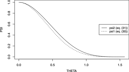
Figure 1: The Gaspari and Cohn (1999) localization function with Euclidean or chordal distance ($\psi_{1}$; eq. (30)), and with spherical or great circle distance ($\psi_{2}$; eq. (31)), as argument.

than the traditional choice, $\psi_{1}$. Similar comments apply to covariance tapers in spatial statistics, as proposed by Furrer, Genton and Nychka (2006).

4.2 Criteria of Pólya type

Criteria of Pólya type provide simple sufficient conditions for positive definiteness, by imposing convexity conditions on a candidate function and/or its higher derivatives. Gneiting (2001) reviews and develops Pólya criteria on Euclidean spaces. In what follows, we are concerned with analogues on spheres that complement the recent work of Beatson, zu Castell and Xu (2011).

The following theorem summarizes results of Wood (1995), Gneiting (1998b) and Beatson, zu Castell and Xu (2011) in the case of the circle $\mathbb{S}^{1}$.

Theorem 4

Suppose that the function $\psi:[0,\pi]\to\mathbb{R}$ is continuous, nonincreasing and convex with $\psi(0)=1$ and $\int_{0}^{\pi}\psi(\theta)\,\mathrm{d}\theta\geq 0$. Then $\psi$ belongs to the class $\Psi_{1}$. It belongs to the class $\Psi_{1}^{+}$ if it is not piecewise linear.

Our next result is a Pólya criterion that applies on spheres $\mathbb{S}^{d}$ of dimension $d\leq 3$. Its proof relies on the subsequent lemmas, the first of which is well known.

Theorem 5

Suppose that $\varphi:[0,\infty)\to\mathbb{R}$ is a continuous function with $\varphi(0)=1$, $\lim_{t\to\infty}\varphi(t)=0$ and a continuous derivative $\varphi^{\prime}$ such that $-\varphi^{\prime}(t^{1/2})$ is convex for $t>0$. Then the restriction $\psi=\varphi_{[0,\pi]}$ belongs to the class $\Psi_{3}^{+}$.

To give an example, we may conclude from Theorem 5 that the truncated power function (27) with shape parameter $\tau\geq 2$ belongs to the class $\Psi_{3}^{+}$ for all values of the support parameter $c>0$, including the case $c>\pi$, in which it is supported globally.

Lemma 1

Let $d\geq 1$ be an integer. Suppose that $C$ is a subset of a Euclidean space, and let $P$ be a Borel probability measure on $C$. If $\psi_{c}$ belongs to the class $\Psi_{d}$ for every $c\in C$, then the function $\psi$ defined by

$$\psi(\theta)=\int_{C}\psi_{c}(\theta)\,\mathrm{d}P(c)\quad\mbox{for}\quad\theta\in[0,\pi]$$

belongs to the class $\Psi_{d}$, too. If furthermore $\psi_{c}$ belongs to $\Psi_{d}^{+}$ for every $c$ in a set of positive $P$-measure, then $\psi$ belongs to the class $\Psi_{d}^{+}$.

Lemma 2

For all $c>0$, the function defined by

$$\psi_{c}(\theta)=\biggl{(}1+\frac{1}{2}\frac{\theta}{c}\biggr{)}\biggl{(}1-\frac{\theta}{c}\biggr{)}_{+}^{2}\quad\mbox{for}\quad\theta\in[0,\pi]$$ (32)

belongs to the class $\Psi_{3}^{+}$.

Proof.

By Theorem 3, the function $\psi_{c}$ belongs to the class $\Psi_{3}^{+}$ if $c\leq\pi$. If $c\geq\pi$, the formulas in (14) yield the Fourier cosine coefficients

$$b_{0,1}=\frac{1}{8c^{3}}\bigl{(}8c^{3}-6\pi c^{2}+\pi^{3}\bigr{)}\qquad\mbox{and}\qquad b_{2k,1}=\frac{3\pi}{4c^{3}}\frac{1}{k^{2}}$$

for all integers $k\geq 1$. Similarly, we find that

$$b_{2k+1,1}=\frac{3}{\pi c^{3}}\biggl{(}\frac{2c^{2}-\pi^{2}}{(2k+1)^{2}}+\frac{4}{(2k+1)^{4}}\biggr{)}$$

for all integers $k\geq 0$ and conclude from part (a) of Corollary 4 that $\psi_{c}$ belongs to $\Psi_{3}^{+}$. ∎

Proof of Theorem 5 By Theorem 3.1 of Gneiting (1999b), the function $\varphi$ admits a representation of the form

$$\varphi(t)=\int_{(0,\infty)}\varphi_{c}(t)\,\mathrm{d}F(c)\quad\mbox{for}\quad t\geq 0,$$

where $\varphi_{c}$ is defined by

$$\varphi_{c}(t)=\biggl{(}1+\frac{1}{2}\frac{t}{c}\biggr{)}\biggl{(}1-\frac{t}{c}\biggr{)}_{+}^{2}\quad\mbox{for}\quad t\geq 0,$$ (33)

and $F$ is a probability measure on $(0,\infty)$. Therefore, the restriction $\psi=\varphi_{[0,\pi]}$ is of the form

$$\psi(\theta)=\int_{(0,\infty)}\psi_{c}(\theta)\,\mathrm{d}F(c)\quad\mbox{for}\quad\theta\in[0,\pi],$$

where $\psi_{c}$ is defined by (32). By Lemma 2, the function $\psi_{c}$ belongs to the class $\Psi_{3}^{+}$ for all $c>0$, and so we conclude from Lemma 1 that $\psi$ is in $\Psi_{3}^{+}$.

Our next theorem is a slight generalization of the key result in Beatson, zu Castell and Xu (2011). In analogy to the corresponding results on Euclidean spaces (Gneiting, 1999b), the case $n=1$ yields a more concise, but less general, criterion than Theorem 5.

Theorem 6

Let $n\leq 3$ be a positive integer. Suppose that $\varphi:[0,\infty)\to\mathbb{R}$ is a continuous function with $\varphi(0)=1$, $\lim_{t\to\infty}\varphi(t)=0$ and a derivative $\varphi^{(n)}$ of order $n$ such that $(-1)^{n}\varphi^{(n)}(t)$ is convex for $t>0$. Then the restriction $\psi=\varphi_{[0,\pi]}$ belongs to $\Psi_{2n+1}^{+}$.

In a recent tour de force, Beatson, zu Castell and Xu (2011) demonstrate the following remarkable result, which is the key to proving Theorem 6.

Lemma 3

Let $n\leq 3$ be a positive integer, and suppose that $c\in(0,\pi]$. Then the function defined by

$$\psi_{c,n}(\theta)=\biggl{(}1-\frac{\theta}{c}\biggr{)}_{+}^{n+1}\quad\mbox{for}\quad\theta\in[0,\pi]$$ (34)

belongs to the class $\Psi_{2n+1}^{+}$.

The next lemma concerns the case $c>\pi$, in which the truncated power function (34) is supported globally.

Lemma 4

For all integers $n\geq 1$ and all real numbers $c\geq\pi$, the function $\psi_{c,n}$ in (34) belongs to the class $\Psi_{\infty}^{+}$.

Proof.

By a convolution argument due to Fuglede (Hjorth et al., 1998, p. 272), the function $\psi_{\pi,0}(\theta)=1-\frac{\theta}{\pi}$ belongs to the class $\Psi_{\infty}$. As the class $\Psi_{\infty}$ is convex and closed under products, we see that if $n\geq 0$ is an integer and $c\geq\pi$ then

$$\psi_{c,n}(\theta)=\biggl{(}\biggl{(}1-\frac{\pi}{c}\biggr{)}+\frac{\pi}{c}\psi_{\pi,0}(\theta)\biggr{)}^{n+1}\quad\mbox{for}\quad\theta\in[0,\pi],$$

whence $\psi_{c,n}$ is in the class $\Psi_{\infty}$, too. By a straightforward direct calculation, the Fourier cosine coefficients of $\psi_{c,1}$ and $\psi_{c,2}$ are strictly positive for all $c\geq\pi$. Therefore, by Theorem 1 of Xu and Cheney (1992) and the fact that the class $\Psi_{1}^{+}$ is closed under products, the function $\psi_{c,n}$ is in the class $\Psi_{1}^{+}$ for all integers $n\geq 1$ and all $c\geq\pi$. Using part (a) of Corollary 1, we conclude that $\psi_{c,n}\in\Psi_{\infty}^{+}$ for all integers $n\geq 1$ and all $c\geq\pi$. ∎

Proof of Theorem 6 By Theorem 3.1 of Gneiting (1999b), the function $\varphi$ admits a representation of the form

$$\varphi(t)=\int_{(0,\infty)}\varphi_{c,n}(t)\,\mathrm{d}F(c)\quad\mbox{for}\quad t\geq 0,$$

where the function $\varphi_{c,n}:[0,\infty)\to\mathbb{R}$ is defined by $\varphi_{c,n}(t)=(1-\frac{\theta}{c})^{n+1}$ for $t\geq 0$ and $F$ is a probability measure on $(0,\infty)$. Therefore, the restriction $\psi=\varphi_{[0,\pi]}$ is of the form

$$\psi(\theta)=\int_{(0,\infty)}\psi_{c,n}(\theta)\,\mathrm{d}F(c)\quad\mbox{for}\quad\theta\in[0,\pi],$$

where $\psi_{c,n}$ is given by (34). By Lemmas 3 and 4, the function $\psi_{c,n}$ belongs to the class $\Psi_{2n+1}^{+}$ for all $c>0$. Therefore, we conclude from Lemma 1 that $\psi$ is in $\Psi_{2n+1}^{+}$, too.

Beatson, zu Castell and Xu (2011) conjectured that the statement of Lemma 3 holds for all integers $n\geq 1$. In view of Lemma 4, if their conjecture is true, the statement of Theorem 6 holds for all integers $n\geq 1$, too, with the proof being unchanged.

It is interesting to observe that Theorem 6 is a stronger result than Theorem 1.3 in Beatson, zu Castell and Xu (2011), in that it does not impose any support conditions on the candidate function $\psi$. In contrast, the latter criterion requires $\psi$ to be locally supported. Such an assumption also needs to made in the spherical analogue of Theorem 1.1 in Gneiting (2001), which we state and prove in Appendix A in the supplemental article (Gneiting, 2013).

4.3 Completely monotone functions

A function $\varphi:[0,\infty)\to\mathbb{R}$ is completely monotone if it possesses derivatives $\varphi^{(k)}$ of all orders with $(-1)^{k}\varphi^{(k)}(t)\geq 0$ for all integers $k\geq 0$ and all $t>0$. Our next result shows that the restrictions of completely monotone functions belong to the class $\Psi_{\infty}^{+}$.

Theorem 7

Suppose that the function $\varphi:[0,\infty)\to\mathbb{R}$ is completely monotone with $\varphi(0)=1$ and not constant. Then the restriction $\psi=\varphi_{[0,\pi]}$ belongs to the class $\Psi_{\infty}^{+}$.

Proof.

Let $a>0$ and consider the truncated power function (34). By Lemma 4, $\psi_{n/a,n}$ belongs to the class $\Psi_{\infty}^{+}$ for all sufficiently large integers $n$. Hence, the function $\psi_{a}$ defined by

$$\psi_{a}(\theta)=e^{-a\theta}=\lim_{n\to\infty}\psi_{n/a,n}(\theta)\quad\mbox{for}\quad\theta\in[0,\pi]$$

belongs to the class $\Psi_{\infty}$, too. By Theorem 5, $\psi_{a}\in\Psi_{3}^{+}$, which in view of part (a) of Corollary 1 implies that $\psi_{a}\in\Psi_{\infty}^{+}$. Now suppose that the function $\varphi:[0,\infty)\to\mathbb{R}$ satisfies the conditions of the theorem. Invoking Bernstein’s Theorem, we see that $\varphi$ admits a representation of the form

$$\varphi(t)=\int_{[0,\infty)}e^{-at}\,\mathrm{d}F(a)\quad\mbox{for}\quad t\geq 0,$$

where $F$ is a probability measure on $[0,\infty)$. Therefore, the restriction $\psi=\varphi_{[0,\pi]}$ is of the form

$$\psi(\theta)=\int_{[0,\infty)}e^{-a\theta}\,\mathrm{d}F(a)=\int_{[0,\infty)}\psi_{a}(\theta)\,\mathrm{d}F(a)\quad\mbox{for}\quad\theta\in[0,\pi].$$

Since $\varphi$ is not constant, $F$ has mass away from the origin. As $\psi_{a}$ is in the class $\Psi_{\infty}^{+}$ for all $a>0$, we conclude from Lemma 1 that $\psi$ belongs to the class $\Psi_{\infty}^{+}$. ∎

Miller and Samko (2001) present a wealth of examples of completely monotone functions, which thus can serve as correlation functions or radial basis functions on spheres of any dimension.

4.4 Necessary conditions

The next result states conditions that prohibit membership in the class $\Psi_{1}$, and therefore in any of the classes $\Psi_{d}$. Heuristically, the common motif can be paraphrased as follows:

If a positive definite function admits a certain degree of smoothness at the origin, it admits the same degree of smoothness everywhere.

The conditions in parts (a) through (d) of the following theorem can be interpreted as formal descriptions of circumstances under which this overarching principle is violated. Part (a) corresponds to a well-known result in the theory of characteristic functions, parts (b) and (c) are due to Wood (1995) and Gneiting (1998b), respectively, and part (d) rests on a result in Devinatz (1959).

Theorem 8

Suppose that the function $\psi:[0,\pi]\to\mathbb{R}$ can be represented as the restriction $\psi=\phi_{[0,\pi]}$ of an even and continuous function $\phi:\mathbb{R}\to\mathbb{R}$ that satisfies any of the following conditions.

• [(a)]

• For some integer $k\geq 1$ the derivative $\phi^{(2k)}(0)$ exists, but $\phi$ fails to be $2k$ times differentiable on $(0,\pi)$.

• For some integer $k\geq 1$, the function $\phi$ is $2k-1$ times continuously differentiable on $[-\pi,\pi]$ with $\phi^{(2k-1)}(\pi)\not=0$ and $|\phi^{(2k-1)}(t)|\leq b_{1}|t|^{\beta_{1}}$ for some $b_{1}>0$ and $\beta_{1}>0$, and is $2k+1$ times continuously differentiable on $[-\pi,0)\cup(0,\pi]$ with $|\phi^{(2k+1)}(t)|\leq b_{2}|t|^{-\beta_{2}}$ for some $b_{2}>0$ and $\beta_{2}\in(1,2)$.

• For some integer $k\geq 1$, the function $\phi$ is $2k$ times differentiable on $[-\pi,\pi]$ with $\phi^{(j)}(\pi)\not=0$ for some odd integer $j$, where $1\leq j\leq 2k-1$.

• The function $\phi$ is analytic and not of period $2\pi$.

Then $\psi$ does not belong to the class $\Psi_{1}$.

An important caveat is the possibly surprising fact that, given some function $\varphi:[0,\infty)\to\mathbb{R}$, the mapping $\psi_{c}:[0,\pi]\to\mathbb{R}$ defined by

$$\psi_{c}(\theta)=\varphi\biggl{(}\frac{\theta}{c}\biggr{)}\quad\mbox{for}\quad\theta\in[0,\pi]$$

may belong to the class $\Psi_{d}$ for some specific values of the scale parameter $c>0$ only, rather than for all $c>0$. For example, the $C^{2}$- and $C^{4}$-Wendland functions in Table 1 allow for $c\in(0,\pi]$ only, with part (c) of Theorem 8 excluding the case $c>\pi$.

A notable exception occurs when $\varphi$ is completely monotone with $\varphi(0)=1$ and not constant. Then the mapping $t\mapsto\varphi(t/c)$ is completely monotone for all $c>0$, and we conclude from Theorem 7 that $\psi_{c}\in\Psi_{\infty}^{+}$ for all values of the scale parameter $c>0$. The first four entries in Table 1 are of this type and will be discussed below.

4.5 Examples

We now apply the criteria of Sections 4.3 and 4.4 to study parametric families of globally supported correlation functions and radial basis functions on spheres. In doing so, we think of $c>0$ as a scale or support parameter, $\alpha>0$ or $\nu>0$ as a smoothness parameter and $\tau>0$ as a shape parameter.

We consider the families in Table 2, namely the powered exponential, Matérn, generalized Cauchy and Dagum classes. For the parameter values stated in Table 2 these families serve as isotropic correlation functions on Euclidean spaces, where the argument is the Euclidean distance. Investigating whether they can serve as isotropic correlation functions with spherical or great circle distance on $\mathbb{S}^{d}$ as argument, we supplement and complete results of Huang, Zhang and Robeson (2011) in the case $d=2$, as summarized in the first four entries of Table 1. In Examples 1 and 2, the results and proofs do not depend on the scale parameter $c>0$, and so we only discuss the smoothness parameter $\alpha$ or $\nu$, respectively.

Example 1 ((Powered exponential family)).

The members of the powered exponential family are of the form

$$\psi(\theta)=\exp\biggl{(}-\biggl{(}\frac{\theta}{c}\biggr{)}^{\alpha}\biggr{)}\quad\mbox{for}\quad\theta\in[0,\pi].$$ (35)

If $\alpha\in(0,1]$, a straightforward application of Theorem 7 shows that $\psi\in\Psi_{\infty}^{+}$. If $\alpha>1$, we see from parts (b) and (c) of Theorem 8 that $\psi$ does not belong to the class $\Psi_{1}$, where part (b) applies when $\alpha\in(1,2)$, and part (c) when $\alpha\geq 2$, both using $k=1$. Therefore, if $\alpha>1$ then $\psi$ does not belong to any of the classes $\Psi_{d}$.

Example 2 ((Matérn family)).

The members of the Matérn family can be written as

$$\psi(\theta)=\frac{2^{\nu-1}}{\Gamma(\nu)}\biggl{(}\frac{\theta}{c}\biggr{)}^{\nu}K_{\nu}\biggl{(}\frac{\theta}{c}\biggr{)}\quad\mbox{for}\quad\theta\in[0,\pi],$$ (36)

where $K_{\nu}$ denotes the modified Bessel function of the second kind of order $\nu$. If $\nu=n+\frac{1}{2}$, where $n\geq 0$ is an integer, then $\psi$ equals the product of $\exp(-\theta/c)$ and a polynomial of degree $n$ in $\theta$ (Guttorp and Gneiting, 2006).

If $\nu\in(0,\frac{1}{2}]$, then $\psi$ belongs to the class $\Psi_{\infty}^{+}$. Indeed, by Theorem 5 of Miller and Samko (2001) the function $\phi_{1}(t)=\exp(t)t^{\nu}K_{\nu}(t)$ is completely monotone if $\nu\leq\frac{1}{2}$. By Theorem 1 of Miller and Samko (2001) the function $\phi_{0}(t)=\exp(-t)\phi_{1}(t)=t^{\nu}K_{\nu}(t)$ is completely monotone, too. In view of Theorem 7, this proves our claim.

If $\nu>\frac{1}{2}$, then $\psi$ does not belong to the class $\Psi_{1}$, and thus neither to any of the classes $\Psi_{d}$. If $\nu\in(\frac{1}{2},1)$, this follows from an application of the estimates in Section 10.31 of Digital Library of Mathematical Functions (2011) to part (b) of Theorem 8, where $k=1$, $\beta_{1}=2\nu-1$ and $\beta_{2}=2\nu-3$. If $\nu\geq 1$, we apply part (c) of Theorem 8, where $k=1$.

In our next example, the results do not depend on the scale parameter $c>0$ and the shape parameter $\tau>0$, and so we discuss the smoothness parameter $\alpha$ only.

Example 3 ((Generalized Cauchy family)).

The members of the generalized Cauchy family are of the form

$$\psi(\theta)=\biggl{(}1+\biggl{(}\frac{\theta}{c}\biggr{)}^{\alpha}\biggr{)}^{-\tau/\alpha}\quad\mbox{for}\quad\theta\in[0,\pi].$$ (37)

If $\alpha\in(0,1]$, a straightforward application of Theorem 7 shows that $\psi$ is a member of the class $\Psi_{\infty}^{+}$. However, if $\alpha>1$ the function $\psi$ in (37) does not belong to the class $\Psi_{1}$. If $\alpha\in(1,2)$, this is evident from part (b) of Theorem 8, where $k=1$, $\beta_{1}=\alpha-1$ and $\beta_{2}=\alpha-3$. If $\alpha\geq 2$ we apply part (c) of Theorem 8, where $k=1$.

Example 4 ((Dagum family)).

The members of the Dagum family are of the form

$$\psi(\theta)=1-\biggl{(}\biggl{(}\frac{\theta}{c}\biggr{)}^{\tau}\bigg{/}\biggl{(}1+\frac{\theta}{c}\biggr{)}^{\tau}\biggr{)}^{\alpha/\tau}\quad\mbox{for}\quad\theta\in[0,\pi].$$ (38)

Using a comment by Berg, Mateu and Porcu (2008, p. 1146) along with Theorem 7, we see that if $c>0$, $\tau\in(0,1]$ and $\alpha\in(0,\tau)$ then $\psi$ is a member of the class $\Psi_{\infty}^{+}$.

Another example that involves oscillating trigonometric and Bessel functions is given in Appendix B in the supplemental article (Gneiting, 2013).

In the context of isotropic random fields and random particles, the smoothness properties of the associated random surface are governed by the behavior of the correlation function at the origin. Specifically, if a function $\psi\in\Psi_{2}$ admits the relationship (8) for some $\alpha\in(0,2]$, the corresponding Gaussian sample paths on the two-dimensional sphere have fractal or Hausdorff dimension $3-\frac{\alpha}{2}$ almost surely (Hansen, Thorarinsdottir and Gneiting, 2011). In this sense, the results in the above examples are restrictive, in that the smoothness parameter needs to satisfy $\alpha\leq 1$ or $\nu\leq\frac{1}{2}$, respectively. Parametric families of correlation functions that admit the full range of viable Hausdorff dimensions include the sine power family (17) and the convolution construction in Section 4.3 of Hansen, Thorarinsdottir and Gneiting (2011). Alternatively, Yadrenko’s construction (7) can be applied to any of the parametric families in Table 2.

5 Challenges for future work

In this paper, we have reviewed and developed characterizations and constructions of isotropic positive definite functions on spheres, and we have applied them to provide rich parametric classes of such functions. Some of the key results in the practically most relevant cases of one-, two- and three-dimensional spheres are summarized in Table 1. Whenever required, the closure properties of the classes of the positive definite or strictly positive definite functions offer additional flexibility. For example, while all entries in Table 1 yield nonnegative correlations only, we can easily model negative correlations, by using convex sums or products of an entry in the table with a suitable Gegenbauer function, such as $\psi(\theta)=\cos\theta$, which belongs to the class $\Psi_{\infty}^{-}$.

Despite substantial advances in the study of positive definite functions on spheres, many interesting and important questions remain open. Therefore, Appendix C in the supplemental article (Gneiting, 2013) describes 18 research problems that aim to stimulate future research in mathematical analysis, probability theory and spatial statistics. The problems vary in scope and difficulty, range from harmonic analysis to statistical methodology, and include what appear to be tedious but routine questions, such as Problem 1, along with well known major challenges, such as Problems 14 through 16, which have been under scrutiny for decades. The first eight problems are of an analytic character and concern the characterization and breadth of the classes $\Psi_{d}$ and $\Psi_{d}^{+}$. Then we state open questions about the parameter spaces for various types of correlation models, relate to the fractal index and the sample path properties of Gaussian random fields, and turn to challenges in spatial and spatio-temporal statistics.

References

- Adler (2009) {bbook}[author] \bauthor\bsnmAdler, \bfnmRobert J.\binitsR.J. (\byear2009). \btitleThe Geometry of Random Fields, \beditionSIAM Classics ed. \blocationPhiladelphia: \bpublisherSIAM. \bptokimsref \endbibitem
- Askey (1973) {bmisc}[author] \bauthor\bsnmAskey, \bfnmR.\binitsR. (\byear1973). \bhowpublishedRadial characteristic functions. Technical Report no. 1262, Mathematics Research Center, Univ. Wisconsin–Madison. \bptokimsref \endbibitem
- Askey and Fitch (1969) {barticle}[mr] \bauthor\bsnmAskey, \bfnmRichard\binitsR. &\bauthor\bsnmFitch, \bfnmJames\binitsJ. (\byear1969). \btitleIntegral representations for Jacobi polynomials and some applications. \bjournalJ. Math. Anal. Appl. \bvolume26 \bpages411–437. \bidissn=0022-247X, mr=0237847 \bptokimsref \endbibitem
- Banerjee (2005) {barticle}[mr] \bauthor\bsnmBanerjee, \bfnmSudipto\binitsS. (\byear2005). \btitleOn geodetic distance computations in spatial modeling. \bjournalBiometrics \bvolume61 \bpages617–625. \biddoi=10.1111/j.1541-0420.2005.00320.x, issn=0006-341X, mr=2140936 \bptokimsref \endbibitem