Enhancing the spreading of quantum walks on star graphs by additional bonds

Abstract

We study the dynamics of continuous-time quantum walks (CTQW) on networks with highly degenerate eigenvalue spectra of the corresponding connectivity matrices. In particular, we consider the two cases of a star graph and of a complete graph, both having one highly degenerate eigenvalue, while displaying different topologies. While the CTQW spreading over the network - in terms of the average probability to return or to stay at an initially excited node - is in both cases very slow, also when compared to the corresponding classical continuous-time random walk (CTRW), we show how the spreading is enhanced by randomly adding bonds to the star graph or removing bonds from the complete graph. Then, the spreading of the excitations may become very fast, even outperforming the corresponding CTRW. Our numerical results suggest that the maximal spreading is reached halfway between the star graph and the complete graph. We further show how this disorder-enhanced spreading is related to the networks’ eigenvalues.

I Introduction

Transfer processes play a very important role in many physical, chemical or biological instances, involving energy, mass or charge. Such transport processes strongly depend on the topology of the system under study, as, for instance in simple crystals ziman1979principles , complex molecules kenkre1982exciton or spin networks burgarth2008coupling .

One often encounters regular networks, such as lattices or rings, where most or all of the nodes have the same degree. Examples are the star graphs (SG), and the complete graphs (CG), which have attracted lately much attention in the field of quantum computation. Such studies focused on the quantum central limit theorem for continuous-time quantum walks on SG salimi2009continuous , the discrete-time Grover walk on a SG with one loop machida2011discrete , and quantum searches on highly symmetric (complete) graphs PhysRevA.79.012323 . Exact analytical results were recently obtained for quantum walks on SG and on CG whose Hamiltonians have one highly degenerate eigenvalue. This, as also discussed in what follows, may let the quantum walk remain localized at its starting node, which then renders the quantum spreading slow.

Spreading of an excitation can be made faster by randomly adding (deleting) bonds to the SG (from the CG). Here we do not allow the additional bonds to connect one node with itself and forbid double bonds between any pair of nodes. The inclusion of the additional bonds changes the structure of the network and, consequently, the eigenvalue set of the corresponding Hamiltonian. Furthermore, destroying the original regularity of the SG (CG), the additional bonds create “shortcuts“ in the graph, by which the spreading through CTQW may occur faster, as, for instance, found for small-world networks mülken2007quantum .

For modelling transport processes on networks one can use several approaches: in quantum mechanics, the Hamiltonian is determined by the connectivity of the system. For example, the dynamics of an electron in a crystal can be described by the Bloch ansatz ziman1979principles . This can be also related to transport processes in polymers, where the connectivity plays an important role in the dynamics doi1988theory .

Classical transport processes modelled by continuous-time random walks (CTRW) are described by a master equation, involving a transfer operator $\bf T$ based on the topology of the system kenkre1982exciton , van1992stochastic , JKempe . A quantum mechanical analogue of CTRW, namely, one variant of the continuous-time quantum walk (CTQW), can be introduced by using the transfer operator $\bf T$ in defining the Hamiltonian $\bf H$ farhi1998quantum . For simple lattices this is equivalent to a nearest-neighbor hopping model farhi1998quantum , mülken2006coherent , mülken2005spacetime , mülken2005asymmetries . The transformation replaces the classical diffusion process by a quantal propagation through the structure.

The paper is organized as follows. Section II introduces the CTRW and CTQW concepts. Tools for determining their spreading are displayed in Section III. Section IV focuses on CTRW and CTQW on SG and on CG, whereas the spreading over graphs intermediate between the SG and the CG is studied in Section V. Section VI concludes with a summary of results.

II Quantum walks on networks

In the following we focus on the dynamics of excitations over networks; these consist of $N$ nodes connected by bonds. The information about a network’s topology, i.e., its connectivity, is stored in the $N\times N$ connectivity matrix $\bf A$, whose elements $A_{kj}$ are:

$$A_{kj}=\left\{\begin{array}[]{ll}f_{j}&\mbox{if $k=j$}\\ -1&\mbox{if $k$ and $j$ are directly connected}\\ 0&\mbox{otherwise}.\end{array}\right.$$ (1)

Here $f_{j}$ is the number of bonds emanating from $j$, also referred to as the degree of $j$. The connectivity matrix has the following properties:

1. $\bf A$ is symmetric and real.

2. All its eigenvalues $E_{n}$ are real and non-negative.

If the network is simply connected, $\bf A$ has a single vanishing eigenvalue $E_{\rm{min}}=0$. In order to model the dynamics in the two extreme cases of a purely coherent and of a purely incoherent (diffusive) transport, we employ the concepts of CTQW and of CTRW, respectively. In both cases, the dynamics is largely influenced by the network’s topology, i.e., by $\mathbf{A}$. Now, we depict an excitation localized at node $j$ through the state $|j\rangle$; the ensemble of the $|j\rangle$ states forms an orthonormal basis set $\{|j\rangle,j=1,...,N\}$. In the incoherent CTRW case, the spreading occurs based on the transition rates $\gamma_{kj}$, which denote the probability to go per unit time from $j$ to $k$. Assuming these rates to be the same for all the nodes, i.e., taking $\gamma_{kj}\equiv\gamma$ (and we will set $\gamma=1$ without loss of generality), induces a simple relation between $\mathbf{T}$ and $\mathbf{A}$, namely, $\mathbf{T}=-\mathbf{A}$ van1992stochastic , farhi1998quantum , mulken2011continuous .

In the quantum case, the states $|j\rangle$ span the whole accessible Hilbert space. The time evolution of an excitation initially placed at node $|j\rangle$ is determined by the system’s Hamiltonian $\bf H$; in the approach of Ref. farhi1998quantum used here, the CTQW is directly related to $\bf T$ through $\bf H=-\bf T$ farhi1998quantum , mulken2011continuous . The classical and quantum mechanical probabilities to be in state $|k\rangle$ at time $t$ when starting at $t=0$ from state $|j\rangle$ are then:

$$p_{k,j}(t)=\langle k|\exp{(\mathbf{T}t)}|j\rangle$$ (2)

and $$\pi_{k,j}(t)=\arrowvert\langle\ k|\exp{(-i\mathbf{H}t)}|\ j\rangle\arrowvert^{2},$$ (3)

respectively, where we set in Eq. (3) $\hbar=1$. For $t=0$ both expressions read $p_{k,j}(0)=\pi_{k,j}(0)=\delta_{k,j}$, where $\delta_{k,j}$ is Dirac’s delta-function.

To get from the formal Eqs. (2) and (3) to the explicit solutions for a particular lattice one has to diagonalize $\mathbf{T}$ and $\mathbf{H}$. Given that here the CTQW Hamiltonian $\mathbf{H}$ is the negative of the CTRW transfer matrix $\mathbf{T}$, lets the eigenvalues and eigenvectors of both operators be practically identical. The difference in the dynamics of CTQW and of CTRW is due to the different functional forms of Eq. (2) and of Eq. (3).

III Classical and quantum spreading

While one needs to calculate the eigenvectors (which can become tedious for large networks) for making definite statements on the transition probabilities $p_{k,j}(t)$ and $\pi_{k,j}(t)$, there are quantities - to be defined below - which only depend on the eigenvalues, whose distribution, the density of states (DOS) or spectral density, is given by:

$$\rho(E)=\frac{1}{N}\sum_{n=1}^{N}\delta(E-E_{N}).$$ (4)

The DOS contains information about the system and allows to analyse several features which depend on the network’s topology. For CTRW one such feature is the classical average probability to be (return or remain) at the initially excited node averaged over all possible initial nodes $j$ alexander1982density , bray1988diffusion :

$$\bar{p}(t)=\frac{1}{N}\sum_{j}{p_{j,j}(t)}=\frac{1}{N}\sum_{n=1}^{N}e^{-E_{n}t}.$$ (5)

Hence $\bar{p}(t)$ depends only on the eigenvalues $E_{n}$ of $\bf A$, but not on its eigenvectors $|\phi_{n}\rangle$.

For CTQW, on the other hand, $\bar{\pi}(t)\equiv\frac{1}{N}\sum_{n=1}^{N}\pi_{j,j}(t)$ depends on the eigenvectors $|\phi_{n}\rangle$. However, one can define, in a fashion similar to the classical $\bar{p}(t)$, the quantity mülken2006coherent , mülken2006efficiency ,

$$\bar{\alpha}(t)\equiv\frac{1}{N}\sum_{j=1}^{N}\alpha_{j,j}(t)=\frac{1}{N}\sum_{n=1}^{N}e^{-iE_{n}t}.$$ (6)

Here $\bar{\alpha}(t)$ also depends only on the eigenvalues $E_{n}$. Furthermore, $\arrowvert\bar{\alpha}(t)\arrowvert^{2}$ obeys the Cauchy-Schwarz inequality mülken2006coherent :

$$\bar{\pi}(t)=\frac{1}{N}\sum_{j}\Big{\arrowvert}{\alpha_{j,j}(t)}\Big{\arrowvert}^{2}\geq\Big{\arrowvert}\bar{\alpha}(t)\Big{\arrowvert}^{2}.$$ (7)

Hence $\arrowvert\bar{\alpha}(t)\arrowvert^{2}$ is a lower bound to $\bar{\pi}(t)$. We will use Eqs. (5) and (6) to assess the spreading mülken2006efficiency . Now, classically, a quick decrease of $\bar{p}(t)$ means a quick increase in the probability of finding the excitation away from the initially excited node. We hence infer that the spreading is faster when $\bar{p}(t)$ decreases more quickly. In the quantum case, because of the unitary time evolution, $\bar{\pi}(t)$ and $\arrowvert\bar{\alpha}(t)\arrowvert^{2}$ show oscillations. However, the overall (average) decay of $\bar{p}(t)$ and of $\arrowvert\bar{\alpha}(t)\arrowvert^{2}$ can be used to infer the spreading, say, by focusing on the decay of the envelope of, in particular, $\arrowvert\bar{\alpha}(t)\arrowvert^{2}$ mülken2006efficiency .

For regular $d-$dimensional networks these procedures to assess the spreading have been used and discussed in mülken2006efficiency . The result was that quantum walks over such networks appear to be faster than the classical ones: the envelope of $\arrowvert\bar{\alpha}(t)\arrowvert^{2}$ turns out to decay as $t^{-d}$, whereas $\bar{p}(t)$ decays as $t^{\frac{-d}{2}}$. Evidently, other networks may (and do) behave differently. In such cases we will use the long-time averages

$$P_{\rm RW}\equiv\lim_{T\to\infty}\frac{1}{T}\int\limits_{0}^{T}dt\ \bar{p}(t)$$ (8)

and $$P_{\rm QW}\equiv\lim_{T\to\infty}\frac{1}{T}\int\limits_{0}^{T}dt\ \arrowvert\bar{\alpha}(t)\arrowvert^{2}$$ (9)

in order to extract a time-averaged global spreading measure.

For CTRW, due to the eigenvalue $E_{1}=E_{\rm{min}}=0$, $\bar{p}(t)$ will eventually drop to the equipartition value $1/N$, as one can see by rewriting Eq. (5) as:

$$\bar{p}(t)=\frac{1}{N}+\frac{1}{N}\sum_{n=2}^{N}e^{-E_{n}t}.$$ (10)

It hence follows that $\lim_{T\to\infty}\bar{p}(t)=1/N$ and also that $P_{\rm RW}=1/N$. Thus, in the incoherent case at long times both quantities do not depend on the topology of the considered network. In the quantum case, $\arrowvert\bar{\alpha}(t)\arrowvert^{2}$ oscillates. With Eqs. (6) and (9) it follows:

$$P_{\rm QW} = \lim_{T\to\infty}\frac{1}{T}\int\limits_{0}^{T}dt\sum_{n,n^{\prime}}e^{-i(E_{n}-E_{n^{\prime}})t}$$ (11)

$$= \frac{1}{N^{2}}\sum_{n,n^{\prime}}\delta(E_{n}-E_{n^{\prime}})=\frac{1}{N}\sum_{n}\rho(E_{n})$$

$$= \sum_{E_{n}}[\rho(E_{n})]^{2}.$$

In Eq. (11) $\delta(E_{n}-E_{n^{\prime}})$ is unity if $E_{n}=E_{n^{\prime}}$ and vanishes otherwise. Note that $\sum_{E_{n}}\rho(E_{n})=1$. Thus, the DOS completely determines the long-time average of $\arrowvert\bar{\alpha}(t)\arrowvert^{2}$. For instance, for a ring with an odd number of nodes all eigenvalues are non-degenerate, i. e. there are $N$ different eigenvalues, each with $\rho(E_{n})=1/N$, and therefore in that case $P_{\rm QW}^{\rm ring}=1/N$. The DOS determines hence the CTQW spreading measure $P_{\rm QW}$.

We can rewrite Eqs. (5) and (6) as

$$\bar{p}(t)=\sum_{E_{n}}\rho({E_{n}})e^{-E_{n}t}$$ (12)

and

$$\bar{\pi}(t)\geq\Big{\arrowvert}\sum_{E_{n}}\rho({E_{n}})e^{-iE_{n}t}\Big{\arrowvert}^{2}=|\bar{\alpha}(t)|^{2},$$ (13)

respectively. In general, for a single highly degenerate eigenvalue $E_{m}$, with $\rho({E_{m}})$ of order $\mathcal{O}(1)$, while the other eigenvalues have a DOS at most of order $\mathcal{O}(1/N)$, the average transition amplitude is mülken2006efficiency :

$$\bar{\alpha}(t)=\Big{\{}\rho({E_{m}})e^{-iE_{m}t}+\sum_{E_{n}\neq E_{m}}\rho({E_{n}})e^{-iE_{n}t}\Big{\}},$$ (14)

from which one gets to order $\mathcal{O}(1/{N^{2}})$ the approximate expression:

$$|\bar{\alpha}(t)|^{2}\approx\rho({E_{m}})\Big{\{}\rho({E_{m}})+\sum_{E_{n}\neq E_{m}}\rho({E_{n}})\cos[(E_{m}-E_{n})t]\Big{\}}.$$ (15)

Equation (15) shows that for highly degenerate eigenvalues the lower bound $|\bar{\alpha}(t)|^{2}$ will not decay to zero, but will oscillate about a finite value. This means that for CTQW there is a high probability to remain or to return to the initially excited node. This leads to a slow average spreading for CTQW on such networks. However, for lattices of high dimensions, there is a significant probability that a walker never returns to the origin, thus, the CTQW can get transient darázs2010pólya . In the following we will focus on two particular examples of such networks and on how to overcome the slow spreading.

IV Star graph and complete graph

There exist many networks with highly degenerate eigenvalues. Here, we focus on two specific networks which have both one highly degenerate eigenvalue but vastly different topologies: On the one hand we consider the SG, which is a network consisting of $N$ nodes with a central node connected to $N-1$ leaf nodes, which are not connected to each other (see Fig. 1). Therefore, the central node has degree $N-1$, and each of the leaf nodes has degree $1$. On the other hand we consider the CG, where each of the $N$ nodes is connected to all other $N-1$ nodes (see Fig. 1). Both networks are very “ordered”, in the sense that there is an “exchange” symmetry, meaning that exchanging the positions of any pair of nodes (except for the central node of the SG) leaves the network invariant.

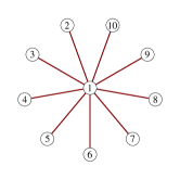
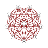
Figure 1: SG and CG of size $N=10$

The connectivity matrices of the two graphs read

$$\bf A_{\rm SG}=\left(\begin{array}[]{lllll}N-1&-1&\cdots&\cdots&-1\\ -1&1&0&\cdots&0\\ \vdots&0&\ddots&&\vdots\\ \vdots&\vdots&&\ddots&0\\ -1&0&\cdots&0&1\end{array}\right)$$ (16)

and

$$\bf A_{\rm CG}=\left(\begin{array}[]{lllll}N-1&-1&\cdots&\cdots&-1\\ -1&N-1&-1&\cdots&-1\\ \vdots&-1&\ddots&&\vdots\\ \vdots&\vdots&&\ddots&-1\\ -1&-1&\cdots&-1&N-1\end{array}\right).$$ (17)

Consequently, the Hamiltonians can be written as

$$\mathbf{H}_{\rm SG}=(N-1)|1\rangle\langle 1|+\sum_{j=2}^{N}{(|j\rangle\langle j|-|1\rangle\langle j|-|j\rangle\langle 1|)}$$ (18)

and

$$\mathbf{H}_{\rm CG}=(N-1)\sum_{j}{(|j\rangle\langle j|)}-\sum_{j\neq i}{(|j\rangle\langle i|)}.$$ (19)

The eigenvalues of both graphs can be calculated analytically. The SG of size $N$ has only three distinct eigenvalues mülken2006efficiency : $E_{1}=0$, $E_{2}=\dots=E_{N-1}=1$, and $E_{N}=N$ and their degeneracies are $D(0)=1$, $D(1)=N-2$, and $D(N)=1$, respectively. The CG of size $N$ has only two distinct eigenvalues xu2009exact , namely $E_{1}=0$ and $E_{2}=\dots=E_{N}=N$, with degeneracies $D(0)=1$ and $D(N)=N-1$.

The dynamics of CTQW and CTRW on SG and on CG has been studied in xu2009exact , where exact analytical results for the transition and the return probabilities have been obtained. It has been shown that when the central node in the SG is initially excited, the spreading turns out to be equivalent to that over a CG of the same size.

Using Eq. (12) and (13) one obtains the following analytical expressions for $\bar{p}(t)$ and for $|\bar{\alpha}(t)|^{2}$ mulken2011continuous for the SG :

$$\bar{p}(t)=\frac{1}{N}\Big{\{}1+(N-2)e^{-t}+e^{-(N-2)t}\Big{\}}$$ (20)

and

$$|\bar{\alpha}(t)|^{2}=\frac{1}{N^{2}}\Big{\arrowvert}1+(N-2)e^{-it}+e^{-i(N-2)t}\Big{\arrowvert}^{2}.$$ (21)

For the CG the analytical expressions for $\bar{p}(t)$ and $|\bar{\alpha}(t)|^{2}$ read mulken2011continuous :

$$\bar{p}(t)=\frac{1}{N}\Big{\{}1+(N-1)e^{-Nt}\Big{\}}$$ (22)

and

$$|\bar{\alpha}(t)|^{2}=\frac{1}{N^{2}}\Big{\arrowvert}1+(N-1)e^{-iNt}\Big{\arrowvert}^{2}.$$ (23)

It is a simple matter to calculate the long-time averages of the expressions above. For Eqs. (20) and (22) the CTRW long-time averages are ${P}_{\rm RW}=1/N$ both for the SG and for the CG. In the quantum case we use $D(E_{n})=N\rho(E_{n})$ in Eq. (11). Such that, using now the explicit eigenvalues and their degeneracies listed above, we obtain:

$$P_{\rm QW}^{\rm SG}=\frac{N^{2}-4N+6}{N^{2}}\geq\frac{1}{N}$$ (24)

and $$P_{\rm QW}^{\rm CG}=\frac{N^{2}-2N+2}{N^{2}}\geq\frac{1}{N}.$$ (25)

We conclude that a quantum walker on such networks in particular for large $N$, has a large probability to stay or to return to the initially excited node, much larger than for a classical walker. We may even see this as a sign that the quantum spreading is slower than its classical analogue. Clearly, this is due to the fact that one eigenvalue of $\mathbf{H}$ is in both cases highly degenerate. One may compare Eqs. (24) and (25) to the situation of a quantum walk over a ring with an odd number of nodes, for which $P_{\rm QW}^{\rm ring}=1/N$. In the latter case there are no degenerate eigenvalues, so that $D(E_{n})=1$ for all $n$. Note that from the value $P_{\rm QW}^{\rm ring}=1/N$ one should not infer that the CTQW is never faster than the CTRW. The result only implies that in the long-time limit the return probability is in average equally distributed among all nodes of the network.

We now turn to the question in how far the situation changes when we (randomly) add bonds to the SG. By this we will explore the transition from the SG to the CG. As it will turn out, the CTQW spreading may increase when the disorder gets larger.

V From the star graph to the complete graph

In this section we consider graphs generated from a SG of size $N$ to which $B$ additional bonds are added. The new bonds are not allowed to connect any node with itself; furthermore only a single bond between any pair of nodes is permitted. The total number of additional bonds, $B_{\rm max}(N)$, needed to convert the SG into the CG of the same size is:

$$B_{\rm max}(N)=\frac{(N-1)(N-2)}{2}.$$ (26)

Examples of SG with $B=3$ additional bonds are given in Figure 2.

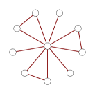
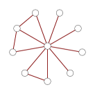
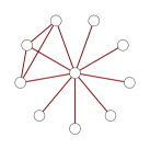
Figure 2: Examples of SG with $B=3$ additional bonds

As seen from Fig. 2, randomly adding bonds to a SG may lead to distinct topologies. While for $B$ very close to $1$ or to $N$ the number of topologically distinct graphs is small, this number increases rapidly when leaving these regions ($B/N\ll 1$ and $(B-N)/N\ll 1$). Now, each topological realization leads to a set of eigenvalues. Graphs with distinct topologies may have an identical set of eigenvalues (the graphs are then called co-spectral cvetkovic1980spectra ). For computational reasons we will not distinguish between such graphs and we will denote by the term ”configuration” the set of graphs leading to the same set of eigenvalues.

We will call the set of all distinct configurations obtained from a SG by adding $B$ additional bonds a “clan”, and denote the number of elements in the clan by $\mathcal{N}_{B}$. Evidently, $\mathcal{N}_{B}$ depends on the size of the network. We determine for every fixed $B$ value the number of distinct eigenvalue sets inside the corresponding clan by considering all the corresponding Hamiltonians. This is done as follows:

1. Generate the Hamiltonian $\bf{H}$ of the given SG (see Eqs. (16) and (18)). There are $(N-1)(N-2)/2$ zero entries above (below) the diagonal (first row and column have only non-zero entries).

2. Consider all the possibilities of changing pairwise such entries from $\mathbf{H}_{ij}=\mathbf{H}_{ji}=0$ to $\mathbf{H}_{ij}=\mathbf{H}_{ji}=-1$, corresponding to the insertion of an additional bond between the nodes $i$ and $j$. There are $2^{\frac{(N-1)(N-2)}{2}}$ ways of doing this, leading to the same number of distinct $\bf H$.

3. For each $\bf{H}$ obtained in this way determine the eigenvalue set and sort the eigenvalues in ascending order.

4. Group together all the $\bf H$ corresponding to a fixed $B$ value and determine by comparison of the ascending eigenvalues the number of distinct eigenvalue sets $\mathcal{N}_{B}$.

For the numerical procedures we use the standard package of Mathematica 8.0. To fix the ideas we start exemplarily with graphs of $N=10$ and with the corresponding clans. We are interested in how many configurations $\mathcal{N}_{B}$ are included in the clan $B$ and how many graphs are represented by a given configuration. For this we show in Table 1 for several $B$ values the corresponding $\mathcal{N}_{B}$.

Moreover, it turns out that a configuration containing graphs which are less symmetric with respect to the exchange symmetry is more probable to show up when distributing the additional $B$ bonds randomly. To exemplify this we also show in Table 1 the most probable and the least probable graph topology together with their eigenvalue sets. One remarkable feature of Table 1 is that the least probable configurations have eigenvalue sets consisting of integer values only, while the eigenvalue sets corresponding to the most probable configurations also include non-integer polynomial roots.

		The least	The most	The least	The most
$B$	$\mathcal{N}_{B}$	probable	probable	probable	probable
		configuration	configuration	eigenvalue	eigenvalue
				set	set
4	11			{10, 5, 3, 3, 1, 1, 1, 1, 1, 0}	{10, 4.414, 3, 3, 1.586,1, 1, 1, 1, 0}
10	1470			{10, 6, 6, 6, 6, 1, 1, 1, 1, 0}	{10, 6.26, 5.4, 4.601, 3.4743, 2.625, 2.5858, 1.705, 1.34, 0}
18	31566			{10, 7, 7, 7, 7, 7, 4, 4, 1, 0}	{10, 8.33, 7.5, 6.395, 5.6087, 5.3913, 4.605, 3.4562, 2.66, 0}
26	1470			{10, 10, 10, 10, 10, 5, 5, 5, 5, 0}	{10, 10, 9.408, 8.8192, 8.353, 7, 6.24, 5.396, 4.7835, 0}
32	11			{10, 10, 10, 10, 10, 10, 8, 8, 6, 0}	{10, 10, 10, 10, 10, 9.4142, 8, 8, 6.5858, 0}

Table 1: For networks of size $N=10$ and different $B$ we display the least and the most probable eigenvalue sets.

Figure 3 shows $\mathcal{N}_{B}$ as a function of $B$ for different $N$. As can be seen from the figure, $\mathcal{N}_{B}$ reaches a maximum around $B(N)=B_{\rm max}(N)/2$. One may note the very large increase of $\mathcal{N}_{B}$ with growing $N$ (note the logarithmic scale on the $y$-axis). For $N=10$ (where $B_{max}=36$) and $B$ taken to be $B_{\rm max}/2=18$ we find more than $3\cdotp 10^{4}$ distinct eigenvalue sets, while for $N=7$ (where $B_{max}=15$) and $B=8$ there are only $215$. For $N$ exceeding $10$ it gets quickly impossible to determine through the above algorithm all the configurations. Thus, for $N\geq 10$ we will rely on randomly creating networks and obtain the ensemble average using a relatively large number $R=10000$ of realizations. Formally we set:

$$\langle...\rangle_{R}\equiv\frac{1}{R}\sum_{r=1}^{R}[...]_{r},$$ (27)

where $r$ runs over the particular realizations. In this way we determine the ensemble-averaged probabilities $\langle\bar{p}(t)\rangle_{R}$ and $\langle|\bar{\alpha}(t)|^{2}\rangle_{R}$, along with the long-time average $\langle P_{\rm QW}\rangle_{R}$.

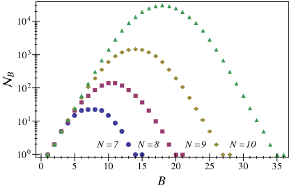
Figure 3: Number of distinct eigenvalue sets as a function of $B$ for the networks of $N=7$, $N=8$, $N=9$, and $N=10$ nodes. Note the logarithmic scale.

V.1 Average probability of being at the origin

The influence of additional bonds on the spreading is captured in the behavior of the transition probabilities between certain pairs of nodes. However, as can be anticipated, the functional form of these transition probabilities strongly depends on the particular nodes chosen. Therefore, we start by considering the ensemble averages of the average probability to be (return or stay) at the initial node. In particular, we focus on the ensemble average of $\bar{p}(t)$ for CTRW and of the lower bound $|\bar{\alpha}(t)|^{2}$ for CTQW, see Eqs. (5) and (6). Taking the time-average of $\langle|\bar{\alpha}(t)|^{2}\rangle_{R}$ yields $\langle P_{\rm QW}\rangle_{R}$, see Eq. (9). Here and in the following we focus on graphs with $N=10$.

Figure 4 shows $\langle P_{\rm QW}\rangle_{R}$ as a function of the number of additional bonds. Clearly, one observes a decrease from the SG-value to a broad minimal plateau centered around $B=B_{\rm max}/2$ (see the inset), after which the values increase again until the CG-value is reached. The minimal value of $\langle P_{\rm QW}\rangle_{R}$ at $B=B_{\rm max}/2$ approaches $1/N$ from above. Therefore, when the number of additional bonds is so large as to yield the maximal number of possible configurations, the time-averaged spreading becomes comparable to that for the corresponding CTRW. From this we can already infer that adding (removing) bonds to (from) the SG (CG) enhances the spreading of CTQW. This behavior differs from the one found for CTQW on SWN which are build up from a ring-like configuration; for SWN the spreading becomes slow with increasing $B$ mülken2007quantum .

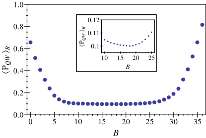
Figure 4: $\langle P_{\rm QW}\rangle_{R}$ for networks of $N=10$ nodes with $R=10000$.

In order to highlight better the behavior of the corresponding CTRW, we have to take a closer look at the temporal development of the average probability to be at the initial node. For the SG and the CG there exist exact analytic expressions for $|\bar{\alpha}(t)|^{2}$ and for $\bar{p}(t)$, see Eqs. (20) and (23). In both cases the lower bound $|\bar{\alpha}(t)|^{2}$ shows oscillations but no decay to a value comparable to $1/N$ (the long-time value for $\bar{p}(t)$). Specifically, $|\bar{\alpha}(t)|^{2}$ oscillates around the values given by Eqs. (24) and (25) for the SG and for the CG, respectively.

Now, on adding bonds to the SG $\langle|\bar{\alpha}(t)|^{2}\rangle_{R}$ follows a complex course: First it decreases to lower values until reaching $B=B_{\rm{max}}/2=18$; then it increases again towards the behavior found for the CG. This is exemplified in Fig. 5 which shows $\langle|\bar{\alpha}(t)|^{2}\rangle_{R}$ for networks of size $N=10$ with $B=4$, $18$, and $32$ additional bonds. One notes that $\langle|\bar{\alpha}(t)|^{2}\rangle_{R}$ for $B=4$ explores roughly the same interval as does $\langle\bar{p}(t)\rangle_{R}$, see Fig. 5(a). Taking $B=B_{\rm max}/2=18$ yields a $\langle|\bar{\alpha}(t)|^{2}\rangle_{R}$ whose time-average is close to $P_{RW}=1/N$ but which also - for short times - reaches values which are about one order of magnitude below those of the CTRW, see Fig. 5(b). Adding more bonds reverses the behavior, i.e., $\langle P_{\rm QW}\rangle_{R}$ becomes larger and the amplitude of the oscillations around this value becomes smaller, see Fig. 5(c).

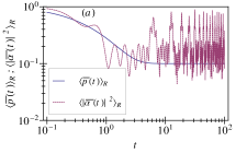
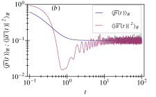
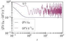
Figure 5: Averaged probabilities $\langle\bar{p}(t)\rangle_{R}$ and $\langle\bar{\pi}(t)\rangle_{R}$ on double logarithmic scales for the SG of size $N=10$ with $B=4$ (a), $18$ (b) and $32$ (c), where $R=10000$.

Since $\langle|\bar{\alpha}(t)|^{2}\rangle_{R}$ is a lower bound, care has to be taken when interpreting the above results. It still might be possible that the exact value, namely $\langle\bar{\pi}(t)\rangle_{R}$, lies above the CTRW curve. However, as has been shown earlier mülken2006efficiency , mulken2011continuous , the maxima of $\langle|\bar{\alpha}(t)|^{2}\rangle_{R}$ tend to be of similar value as the maxima of $\langle\bar{\pi}(t)\rangle_{R}$. In particular, for $B=B_{\rm max}/2$ there is a considerable short-time part (up to $t\approx 4$) where $\langle|\bar{\alpha}(t)|^{2}\rangle_{R}$ lies below $\langle\bar{p}(t)\rangle_{R}$ and which includes several local maxima. Note that at $t\approx 4$ $\langle\bar{p}(t)\rangle_{R}$ has already reached the equipartition value. We thus infer that in this case during the (short) time interval needed by the CTRW to reach equipartition, the spreading of CTQW is faster than that of the corresponding CTRW.

Eigenvalue sets

Both $\langle|\bar{\alpha}(t)|^{2}\rangle_{R}$ for CTQW as well as $\langle\bar{p}(t)\rangle_{R}$ for CTRW depend only on the corresponding eigenvalues (of the Hamiltonian and of the transfer matrix, respectively). As mentioned above, the SG and the CG have eigenvalue sets with one highly degenerate eigenvalue. This situation will change as a function of $B$.

In order to visualize the transition from the SG to the CG in the domain of the eigenvalues, we consider as a function of $B$ the quantity:

$$d_{B}(E)=\langle\sum_{n}\theta(E-E_{n}^{(B)})\rangle_{R}=\frac{1}{R}\sum_{n,r}\theta(E-[E_{n}^{(B)}]_{r}).$$ (28)

Here $\theta(x)$ is the Heaviside function and $E_{n}^{(B)}$ are the eigenvalues of the $r$th realization of the distribution of the $B$ additional bonds. The quantity $d_{B}(E)$ gives the average number of eigenvalues below $E$. Figure 6 shows $d_{B}(E)$ for $B=4,10,18,26$, and $32$.

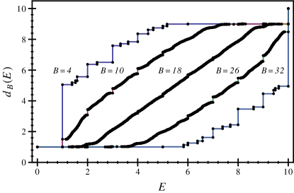
Figure 6: Aveage number of eigenvalues for $N=10$ below $E$; here the number of additional bonds is $B=4,10,18,26$, and $32$, see text for details.

With increasing $B$ the eigenvalues move to higher values, as is evident from the fact that the $d_{B}(E)$ curves decrease with increasing $B$. Sharp steps in $d_{B}(E)$ indicate eigenvalues with large degeneracy; such instances are particularly clear for $B=4$ and for $B=32$ whereas the curve for $B=18$ is much smoother. This is in line with the behavior of $|\bar{\alpha}(t)|^{2}$: a few highly degenerate eigenvalues lead to a plateau in $|\bar{\alpha}(t)|^{2}$ whereas non-degenerate eigenvalues let $|\bar{\alpha}(t)|^{2}$ drop to values close to the CTRW equipartition value $1/N$.

VI Conclusion

We have studied the dynamics of continuous-time quantum walks on networks whose connectivity matrices have one highly degenerate eigenvalue. This fact leads to a slow spreading of CTQW in term of the average probability to return or remain at the initially excited node of the network. In particular, we focused on two types of networks, the star graph and the complete graph. We studied the crossover from the star graph to the complete graph by randomly adding bonds to the star graph until reaching the complete graph. In so doing we found that in the ensemble average the spreading gets faster when adding approximately $B=B_{\rm max}/2$ bonds to the star graph. The reason for this behavior is to be found in the ensemble averaged distribution of the eigenvalues of the connectivity matrices. Adding (extracting) more and more bonds to (from) the star (complete) graph results in broader distributions. Thus, we have shown that under disorder, obtained by either adding bonds to the star graph or by deleting bonds from the complete graph, the quantum walks spread more.

- (1) Alexander, S., Orbach, R.: Density of states on fractals: “fractons”. J. Phys. (Paris) Lett. 43, 625–631 (1982)
- (2) Bray, A., Rodgers, G.: Diffusion in a sparsely connected space: A model for glassy relaxation. Phys. Rev. B 38, 11461 (1988)
- (3) Burgarth, D., Maruyama, K., Nori, F.: Coupling strength estimation for spin chains despite restricted access. Arxiv preprint arXiv:0810.2866 (2008)
- (4) Cvetković, D., Doob, M., Sachs, H.: Spectra of Graphs: Theory and Applications. Academic Press, New York (1997)
- (5) Darázs, Z., Kiss, T.: Pólya number of the continuous-time quantum walks. Phys. Rev. A 81, 062319 (2010)
- (6) Doi, M., Edwards, S.: The theory of polymer dynamics. Oxford University Press, Oxford (1988)
- (7) Farhi, E., Gutmann, S.: Quantum computation and decision trees. Phys. Rev. A 58, 915 (1998)
- (8) van Kampen, N.: Stochastic processes in physics and chemistry. Amsterdam: North Holland (1992)
- (9) Kempe, J.: Quantum random walks - an introductory overview. Contemporary Physics 44, 307 (2003)
- (10) Kenkre, V., Reineker, P.: Exciton dynamics in molecular crystals and aggregates. Springer, Berlin (1982)
- (11) Machida, T.: The discrete-time Grover walk on star graphs with one loop. Arxiv preprint arXiv:1103.1280 (2011)
- (12) Mülken, O., Bierbaum, V., Blumen, A.: Coherent exciton transport in dendrimers and continuous-time quantum walks. J. Chem. Phys. 124, 124905 (2006)
- (13) Mülken, O., Blumen, A.: Spacetime structures of continuous-time quantum walks. Phys. Rev. E 71, 036128 (2005)
- (14) Mülken, O., Blumen, A.: Efficiency of quantum and classical transport on graphs. Phys. Rev. E 73, 066117 (2006)
- (15) Mülken, O., Blumen, A.: Continuous-time quantum walks: Models for coherent transport on complex networks. Phys. Rep. 502, 37 (2011)
- (16) Mülken, O., Pernice, V., Blumen, A.: Quantum transport on small-world networks: A continuous-time quantum walk approach. Phys. Rev. E 76, 051125 (2007)
- (17) Mülken, O., Volta, A., Blumen, A.: Asymmetries in symmetric quantum walks on two-dimensional networks. Phys. Rev. A 72, 042334 (2005)
- (18) Reitzner, D., Hillery, M., Feldman, E., Bužek, V.: Quantum searches on highly symmetric graphs. Phys. Rev. A 79, 012323 (2009)
- (19) Salimi, S.: Continuous-time quantum walks on star graphs. Ann. Phys. 324, 1185–1193 (2009)
- (20) Xu, X.: Exact analytical results for quantum walks on star graphs. J. Phys. A 42, 115205 (2009)
- (21) Ziman, J.: Principles of the Theory of Solids. Cambridge University Press, Cambridge, England (1979)