The scaling properties of exchange and correlation holes of the valence shell of second row atoms

Abstract

We study the exchange and correlation hole of the valence shell of second row atoms using variational Monte Carlo techniques, especially correlated estimates, and norm-conserving pseudopotentials. The well-known scaling of the valence shell provides a tool to probe the behavior of exchange and correlation as a functional of the density and thus test models of density functional theory. The exchange hole shows an interesting competition between two scaling forms – one caused by self-interaction and another that is approximately invariant under particle number, related to the known invariance of exchange under uniform scaling to high density and constant particle number. The correlation hole shows a scaling trend that is marked by the finite size of the atom relative to the radius of the hole. Both trends are well captured in the main by the Perdew-Burke-Ernzerhof generalized-gradient approximation model for the exchange-correlation hole and energy.

I Introduction

Density functional theory Hohenberg and Kohn (1964); Jones and Gunnarsson (1989), the most widely used computational tool for electronic structure calculations, is founded upon the knowledge of the existence of a universal functional mapping the ground-state density to the ground-state energy, with, however, a fundamental lack of knowledge how to construct this functional systematically. The key problem is describing the effects of electron-electron interactions due to Fermi statistics and Coulomb repulsion – the exchange and correlation energies – in an essentially single-particle description of nature. Considerable progress in constructing approximate functionals has been made, using a number of varied strategies to develop a “Jacobs ladder” hierarchy of models of increasing complexity. Two such strategies which have proved fruitful are the discovery and implementation of scaling laws that describe limiting behavior of the universal density functional and the analysis of auxiliary expectations, particularly the exchange-correlation hole, to provide insight into the role of interelectron correlations in determining this functional.

In DFT, scaling laws provide a controlled way of varying density, approaching the daunting task of understanding the energy as a functional of the density by first tackling the more approachable one of understanding its behavior as a function of a scaling variable. Particularly useful is the limit of uniform scaling to high density Levy and Perdew (1985); Levy (1991), a process intimately related to the adiabatic connection approach to DFT Exc , and asymptotically approached by the isoelectronic series of atomic ions as nuclear charge $Z$ tends to infinity. The properties of exchange and correlation under this tranformation constrain the possible dependence of the energy on local-density based variables, greatly simplifying the task of functional construction. Another fruitful scaling process is that of neutral atoms in the $Z\!\rightarrow\!\infty$ limit, in which the charge density tends to a well known Thomas-Fermi limit Scott (1952); March (1957). The gradient correction of the latter has been used to diagnose a major limitation in the widely used generalized gradient approximation (GGA) of DFT, namely the limited ability to tune the GGA to predict accurately both molecular and solid-state properties Perdew et al. (2006), and to motivate effective recent remedies for this issue Perdew et al. (2008, 2009).

Another important tool in the development of DFT has been the exchange-correlation (XC) hole. The XC hole essentially is the measure of the change in electron number density throughout a system given one electron observed to be at a given position. The energy of interaction of an electron with its own exchange-correlation hole yields the exchange-correlation energy, the key theoretical input into DFT. The unexpected degree of success of the original local density approximation (LDA) stems from the universal properties of the system-averaged XC hole (a hole averaged over angle and position in the system) obeyed by the homogeneous electron gas hole Jones and Gunnarsson (1989) from which the LDA is derived. Input from the behavior of the XC hole has been important in the development of effective nonempirical GGA’s Perdew (1991); Perdew et al. (1996); PBE and the hybrid DFT-Hartree Fock approach Becke (1993). More recent DFT models have not been constructed from XC holes, but constructing model XC holes consistent with a given functional remains an important analysis tool Constantin et al. (2006).

The system-averaged exchange-correlation hole has a natural connection to the intracule Coulson and Neilson (1961) or density of electron-pairs as a function of their interelectron distance. The intracule has been the subject of extensive study in quantum chemistry, as a source of insight into the electron correlation problem. Several classes of techniques have been used to study atoms and simple molecules, including Hartree Fock Koga and Matsuyama (1997); Matsuyama et al. (1998); Koga (2000), configuration interaction methods Banyard and Mobbs (1981); Fradera et al. (2000a, b); Wang et al. (1992, 1994); Cioslowski and Liu (1998); *CiosLiu3, and quantum Monte Carlo (QMC) Cancio et al. (2000); Gálvez et al. (2005); *Galvez:044319; Toulouse et al. (2007). Among the many applications include scaling across isoelectronic series Gálvez et al. (2005, 2006), scaling across the periodic table Matsuyama et al. (1998); Koga and Matsuyama (1997); Koga (2000), decomposition into approximate exchange and correlation components Fradera et al. (2000a); Wang et al. (1992, 1994) and shell analysis Banyard and Mobbs (1981); Matsuyama et al. (1998). Pair densities are of additional interest because they can be measured experimentally Thakkar et al. (1984); Wang et al. (1994) and are the basis of some density functional theory approaches Gori-Giorgi and Savin (2005); Nagy (2006).

The decomposition of the intracule into Fermi, or Hartree-Fock hole, and Coulomb hole, incorporating effects from correlations, is a close but imperfect equivalent to exchange and correlation in DFT. The former uses the Hartree-Fock ground-state density as the reference point for defining both Fermi and Coulomb correlations rather than the exact ground-state density as required in DFT. This difference produces a failure of the virial theorem at the level of correlation that can be a ten percent effect in the case of an atom or a major issue in the case of a molecule near dissociation Buijse and Baerends (1995). Secondly, standard Coulomb holes account only for the correlation potential energy. To obtain the correlation contribution to the kinetic energy – the difference between the true and noninteracting-system kinetic energies – an adiabatic integration of the correlation hole with respect to coupling-constant must be performed Exc . Calculations of “true” exchange-correlation holes, using orbitals that reproduce at least the density of one’s correlated wavefunction, have been done mainly in the QMC approach Fahy et al. (1990); Hood et al. (1997, 1998); Nek ; Cancio et al. (2001); Puzder et al. (2001); Hsing et al. (2006).

In this paper, we calculate and analyze the exchange and correlation holes of the valence shell of second row atoms in a pseudopotential model using the variational quantum Monte Carlo (VMC) technique. To our knowledge, this scaling phenomenon has not been studied in the context of density functional theory – although it was an important ingredient in the earliest attempts at a pseudopotential description of atomic structure Slater (1930). Uniform scaling of the radial valence-charge density across a row of the periodic table provides a convenient way to test the idea of “semilocality” of the system-averaged hole by varying the ratio of correlation length to atomic radius over a series of otherwise similar systems. The second row of the periodic table is easy to handle with pseudopotential methods and thus easy to isolate strictly valence properties. The valence density that results is very close to scale-invariant. The systems studied are building blocks of semiconductor materials, and probe a density regime, lower than that of the 1st row valence shell, typical of many solids for which pseudopotential simulations are generally used.

The variational Monte Carlo approach Foulkes et al. (2001) makes feasible the use of explicitly-correlated trial wavefunctions, including the electron-electron cusp condition that affects the pair-density at zero electron-pair separations. To obtain separate system-averaged exchange and correlation holes, we construct single-particle orbitals that reproduce the VMC single-particle density. Exchange holes are then calculated numerically from these orbitals. To reduce the errors from fluctuations in the pair density due to random sampling, correlated estimates techniques are used. These prove important for the measurement of the correlation hole which is a small fraction of the total pair density and thus more affected by noise. The resulting exchange and correlation holes are analyzed with respect to the scaling of the valence shell density across the row and with respect to various density functional models.

The paper is organized as follows. Section II discusses the theoretical underpinnings of the paper – exchange and correlation holes, the GGA approximation, and the scaling of the valence shell. Section III describes the computation techniques used to generate holes and other expectations, Section IV presents our results and Section V our conclusions. All results are expressed in hartree atomic units.

II Theory

II.1 Expectations of interest

The exchange-correlation (XC) hole, $n_{xc}({\bf r},{\bf r}+{\bf u})$, is defined as the reduction in the ground-state electron density from its mean value at some point ${\bf r}\!+\!{\bf u}$ given the observation of an electron at ${\bf r}$. It is obtained from a pair density fluctuation relationship:

$$n({\bf r})n_{xc}({\bf r},{\bf r}+{\bf u})=n^{(2)}({\bf r},{\bf r}+{\bf u})-n({\bf r}+{\bf u})n({\bf r})$$ (1)

where $n({\bf r})$ is the single-particle density, and

$$n^{(2)}({\bf r},{\bf r^{\prime}})=\left\langle\sum_{i}^{N}\sum_{j\neq i}^{N}\delta({\bf r}-{\bf r_{i}})\delta({\bf r^{\prime}}-{\bf r_{j}})\right\rangle.$$ (2)

is the pair density, measuring the expectation of simultaneously finding electrons at ${\bf r}$ and ${\bf r}^{\prime}$. Eq. (1) relates the XC hole to the difference between the actual pair density and that of the uncorrelated system with the same single-particle density.

The utility of the XC hole in density functional theory lies in its relation to the exchange-correlation energy $E_{xc}$ through an adiabatic connection Exc :

$$E_{xc}=\frac{1}{2}\displaystyle\int_{0}^{1}d\lambda\displaystyle\int d^{3}r\displaystyle\int d^{3}u\;\frac{1}{u}n^{\lambda}_{xc}({\bf r},{\bf r}+{\bf u}).$$ (3)

$E_{xc}$ takes into account both the gain in potential energy from creating the exchange-correlation hole about an electron, and, by means of the integration over the coupling constant $\lambda$, the kinetic energy cost of creating the hole as well. The $\lambda$ integral is over a family of systems characterized by the same ground-state density but varying coupling constant $\lambda e^{2}$. A $\lambda$-dependent XC hole $n^{\lambda}_{xc}$ is defined as an expectation of the corresponding ground-state wavefunction. The limits of the integral range from a noninteracting system ($\lambda\!=\!0$), described by the Kohn-Sham equations of DFT Kohn and Sham (1965), to the fully interacting, physical system ($\lambda\!=\!1$).

The $\lambda\!=\!1$ limit which describes the fully interacting Hamiltonian is the focus of this paper. By ignoring the integration over coupling constant, we lose the ability to calculate the correlation kinetic energy and thus lose some of the information contained in the full XC energy. However, we keep the ability to assess DFT models for this quantity since one can use a scaling relation to convert the hole integrated over $\lambda$ into that evaluated at any specific value of $\lambda$. This thereby eliminates a tedious chore for the quantum Monte Carlo method and allows one to explore multiple systems more readily Adi .

As the Coulomb interaction depends only on the interparticle distance $u$, and not on the location or angular orientation of the hole, it is convenient to define a system- and angle-averaged hole,

$$\langle n_{xc}(u)\rangle=\frac{1}{4\pi}\int\!d^{3}r\!\int\!d\Omega_{u}\;n({\bf r})n_{xc}({\bf r},{\bf r}+{\bf u})\;$$ (4)

where $d\Omega_{u}$ is the solid angle of the pair displacement ${\bf u}$. This expression may be normalized by the number of particles $N$ or number of particle pairs $N^{2}$. The system-averaged hole contains that part of the XC hole that directly affects the determination of $E_{xc}$, which simplifies to

$$E_{xc}=\displaystyle\int_{0}^{1}\!d\lambda E_{xc}^{\lambda}=\displaystyle\int_{0}^{1}\!d\lambda\displaystyle\int\!du\;2\pi u\langle n^{\lambda}_{xc}(u)\rangle$$ (5)

because of the isotropy of the Coulomb interaction. The system-averaged hole is closely related to the intracule, defined as:

$$\langle n^{(2)}(u)\rangle=\left\langle\sum_{i\neq j}\delta(u-r_{ij})\right\rangle.$$ (6)

The system-averaged hole is the difference between the intracule of a quantum system and that of the uncorrelated system with the same single-particle density.

The XC hole is usefully decomposed in several ways to isolate various sources of electron correlation. The exchange (X) hole $n_{x}$ is defined as the exchange-correlation hole at zero coupling or $n_{xc}^{\lambda\!=\!0}$. This is the hole associated with the Slater determinant wavefunction that reproduces the ground-state density of the fully interacting system and characterizes the inter-electron correlations due to the Pauli principle. The correlation (C) hole is the difference between the exchange and exchange-correlation holes and measures the additional many-body correlations induced by the Coulomb interaction:

$$\langle n_{c}(u)\rangle=\langle n_{xc}(u)\rangle-\langle n_{x}(u)\rangle.$$ (7)

In addition, it is useful to consider the spin-decomposition of the XC hole, particularly in spin-polarized systems. One may define parallel and anti-parallel-spin holes by restricting the sums in Eq. (2) to particles with the same or opposite spins respectively. The parallel spin hole is dominated by the exchange contribution, since the exchange hole already creates distance between electrons of the same-spin, so that further effects due to correlation are small. On the other hand, the antiparallel spin channel, where the exchange hole is zero, contributes the bulk of the correlation hole.

As it describes the noninteracting system, the spin-decomposed exchange-only hole can be written exclusively in terms of the Kohn-Sham single-particle orbitals that define this limit. The system-averaged hole in this case is obtained exactly as

$$\langle n^{\sigma\sigma}_{x}(u)\rangle=-\int d^{3}r\int\frac{\Omega_{u}}{4\pi}\left|\displaystyle\sum_{i=1}^{N_{\sigma}}\psi_{i\sigma}({\bf r})\psi^{*}_{i\sigma}({\bf r}+{\bf u})\right|^{2}$$ (8)

where

$$\langle n_{x}(u)\rangle=\sum_{\sigma}\langle n^{\sigma\sigma}_{x}(u)\rangle,$$ (9)

and $\psi_{i\sigma}$ are Kohn-Sham orbitals for each spin.

Finally worth noting is that the XC hole obeys the sum rule:

$$\frac{1}{N}\int 4\pi u^{2}du\langle n_{xc}(u)\rangle=-1.$$ (10)

The overall effect of the hole is to remove exactly one particle from the measurement of the density about any given electron, essentially removing self-interaction. Given their respective definitions, the exchange hole must satisfy the same sum rule as exchange-correlation, while the correlation hole, being merely a redistribution of the $N-1$ other electrons around the one in consideration, integrates to zero.

II.2 Exchange-correlation Hole in Semilocal Density Functional Theory

In a “semilocal” density functional theory, the exchange-correlation hole at some point ${\bf r}$ in space is constructed in terms of various observables defined at that point: local spin densities $n_{\uparrow}({\bf r})\!$ and $n_{\downarrow}({\bf r})\!$ in the local spin-density (LSD) variant of the LDA von Barth and Hedin (1972); Jones and Gunnarsson (1989), and adding density gradients $\nabla n_{\uparrow}({\bf r})\!$ and $\nabla n_{\downarrow}({\bf r})\!$ in generalized gradient approximations (GGA’s) PBE ; Becke (1988); Lee et al. (1988); Armiento and Mattsson (2005); Zhao and Truhlar (2008). Kinetic energy densities Becke (1998); Tao et al. (2003); Schmider and Becke (2000); Zhao and Truhlar (2006), and higher-order derivatives of the density such as the Laplacian Lee et al. (1988); Perdew and Constantin (2007); Cancio and Chou (2006) are included in the meta-GGA class of theories.

The LSD exchange-correlation hole at a point ${\bf r}$ is obtained from the pair correlation function $g_{xc}$ of the spin-polarized homogeneous electron gas (HEG):

$$n^{LSD}_{xc}({\bf r},{\bf r}+{\bf u})=n({\bf r})\{g^{HEG}_{xc}\;[u,\,r_{s}({\bf r}),\,\zeta({\bf r})]-1\}.$$ (11)

The pair correlation function is parametrized in terms of the Wigner-Seitz radius $r_{s}$, measuring the average distance between electrons, and the spin polarization $\zeta$, and both are evaluated from the local value of the spin densities:

$$r_{s}({\bf r}) = \left(\frac{3}{4\pi n({\bf r})}\right)^{1/3}$$ (12)

$$\zeta({\bf r}) = \frac{n_{\uparrow}({\bf r})\!-\!n_{\downarrow}({\bf r})}{n({\bf r})}.$$ (13)

The system-averaged hole and total XC energy may then be obtained numerically by applying Eq. (4) and Eq. (5) respectively.

Among the many variants of the GGA in current use, one of particular interest here is that PBE of Perdew, Burke and Ernzerhof (PBE), for which models of $\langle n_{x}(u)\rangle$ Perdew et al. (1996); Ernzerhof and Perdew (1998) and $\langle n_{c}(u)\rangle$ Perdew et al. (1996) have been constructed, building upon an accurate HEG hole Perdew and Wang (1992). Holes within the PBE model are designed, under integration, to reproduce PBE exchange and correlation energies at any value of the density and its gradient within an error of about 5%.

For the exchange hole and energy, the PBE and related models introduce into Eq. (11) a unitless, scale-invariant parameter $s$, defined as

$$s({\bf r})=\frac{1}{2k_{F}({\bf r})}\left|\frac{\nabla n({\bf r})}{n({\bf r})}\right|,$$ (14)

with $k_{F}=(9\pi/4)^{1/3}/r_{s}$ the fermi wavevector. A value of $s$ greater than one at a given point indicates the breakdown of the basic assumption of the LSD that the density varies insignificantly on the length scale $\sim 1/k_{F}$ of the XC hole. For correlation, the PBE employs a second inhomogeneity parameter PBE ,

$$t({\bf r})=\left[k_{F}({\bf r})/\phi(\zeta)k_{s}({\bf r})\right]s({\bf r}),$$ (15)

with the local Thomas-Fermi screening vector, $k_{s}\!=\!(4k_{F}({\bf r})/\pi)^{1/2}$, setting the hole length scale and $\phi(\zeta)$, an additional scaling factor for spin-polarized systems.

As the quantity of interest in this paper is the system averaged hole rather than the local hole, it is helpful to consider system-averages of semilocal DFT parameters. A simple definition of the system-averaged Wigner radius $\langle r_{s}\rangle$ for an atom is Burke et al. (1998)

$$\langle r_{s}\rangle=\displaystyle\frac{\int dr\>r^{2}n(r)^{2}r_{s}(r)}{\int dr\>r^{2}n(r)^{2}},$$ (16)

assuming the pair density for zero interparticle separation Fradera et al. (2000b) is a reasonable measure of the importance of the hole at ${\bf r}$ to energy expectations, and ignoring the anisotropy of the density. System-averaged spin polarization $\langle\zeta\rangle$ and inhomogeneity factors $\langle s^{2}\rangle$ and $\langle t^{2}\rangle$ are similarly defined.

Finally, it is important to note that we are calculatiing the system-averaged correlation hole at full coupling constant ($\lambda\!=\!1$), and with it, the correlation potential energy. DFT models for the correlation hole model the adiabatically integrated hole and thus the total correlation energy. It is possible however to construct the DFT correlation hole and energy density at a given value of coupling constant $\lambda$ from the adiabatically integrated version. This can be derived from the scaling properties of the hole under uniform scaling of the system Perdew and Wang (1992). For the GGA the following expression for the pair correlation function is the result:

$$g_{c}^{1}(r_{s},s,\zeta,k_{F}u)=\bar{g}_{c}(r_{s},s,\zeta,k_{F}u)-\frac{\partial\bar{g}_{c}(r_{s},s,\zeta,k_{F}u)}{\partial\ln{r_{s}}},$$ (17)

with the correlation hole obtained from the expression

$$n_{c}({\bf r},{\bf r}+{\bf u})=n({\bf r})\left[g_{c}({\bf r},u)-1\right],$$ (18)

definable for both $n_{c}^{\lambda}$ and $\bar{n}_{c}$. The parameters $k_{F}u$, $\zeta$, and $s^{2}$ (but not $t^{2}$) are invariant under uniform scaling of position coordinates ${\bf r}_{i}$ (given by ${\bf r}_{i}\!\rightarrow\!{\bf r}_{i}/\lambda$, and $n({\bf r})\!\rightarrow\!n({\bf r}/\lambda)/\lambda^{3}$), and thus held fixed in the derivative. In constrast, the exchange hole is invariant under changes in scale or coupling constant, and is constructed in terms of the scale-independent quantities only.

II.3 Valence Shell Scaling of Atoms

A well-known feature of the periodic table is the scaling of the valence-shell electron density across the 1st or 2nd row atoms (the 2s and 2p or the 3s and 3p atoms respectively). As the number of valence electrons $N$ increases, the shell radius $a(N)$ shrinks with no change in the shape of the distribution:

$$n(r;N)=\frac{N}{a(N)^{3}}\bar{n}[r/a(N)].$$ (19)

The scaling behavior strictly occurs for the valence density outside the core radius. But with the use of pseudopotentials to remove the complicated oscillatory behavior of the valence shell inside the core, this scaling behavior becomes a global feature of the density – one motive for the development of pseudopotentials historically Slater (1930). The radius $a$, usefully defined as the radius of the peak in the radial distribution function $4\pi r^{2}n(r)$, is a function of valence number $N$, so that, if the distribution were perfectly scaling, the density should reduce to a function of $N$ alone across the row. (We consider neutral atoms, with $N=Z_{V}$, the charge of the ion core.) As a result all other expectations of the pseudopotential system ground-state should be reducible to simple functions of $N$, in accordance to the Hohenberg-Kohn theorems Hohenberg and Kohn (1964). Such a picture is limited by the non-scaling behavior of the valence density in the ionic core, not a large contribution to the probability distribution due to the relatively small volume of the core. It is also affected by differences between the Mg atom and atoms with 3p orbitals, and by the open-shell structure of several of the atoms.

Important insights into this scaling can be gained by the simple heuristic shielding model of the atom developed by Slater Slater (1930). This model assumes a self-consistent field felt by an electron in energy shell $i$ given by a shielded Coulomb potential $(Z-\sigma_{i})/r$, with $\sigma_{i}$ the shielding charge felt by the electrons of the shell. The orbitals for principle quantum number $n$ are nodeless Slater-type orbitals $r^{n-1}\exp{[(Z-\sigma_{i})r/n]}$, imposing scaling of the density across a row. The effective Bohr radius – the peak of the radial probability distribution for the valence shell – occurs at

$$a=\frac{a_{0}n^{2}}{Z-\sigma_{V}}=\frac{a_{0}n^{2}}{A+BN},$$ (20)

with $\sigma_{V}$ the valence-shell shielding charge. Slater’s “back-of-the-envelope” rules for determining shielding coefficients yield a shielded effective charge $Z-\sigma_{V}$ that is a linear function of $N$, with coefficients for the valence shell of the 2nd row atoms of $B\!=\!0.65$ and $A\!=\!1.55$.

Energetic quantities can thus be constructed as functions of $N$ from consideration of the scaling form for the density [Eq. (19)] and $a(N)$. The total energy of the valence shell in the Slater model is $(Z-\sigma_{V})N/2a(N)$ in hartrees; expressing the shielding charge in terms of $a(N)$ yielding a scaling dependence of $N/a^{2}$. The kinetic energy in this naive picture scale in the same way, while the external potential due to the ion scales as $N^{2}/a$ for $Z_{V}\!=\!N$. The Hartree or classic electrostatic energy scales as $N(N-1)/a$ provided that self-interaction error is removed. With these scaling assumptions, the virial theorem relating potential and total energy is satisfiable by $a(N)$ taking on the Pade function form of Eq. (20) Sla .

The most interesting energetic quantity for our purposes is the exchange energy. The heuristic picture for scaling of valence-shell energies should be readily extended to the exchange energy, as it in fact obeys an important universal scaling law Levy and Perdew (1985):

$$E_{x}[n_{\alpha}]=\alpha E_{x}[n].$$ (21)

where the density $n_{\alpha}$ is defined by the uniform scaling of $n(r)$ at constant particle number:

$$n_{\alpha}(r)=\alpha^{3}n(\alpha r).$$ (22)

To touch base with the current situation, we note that particle number $N$ is not fixed as one fills up the valence shell, so that the density scales with an additional prefactor $N$, with an $N$-dependent length scale $a(N)$ playing the role of $1/\alpha$. A similar situation is seen in the Thomas Fermi scaling of all-electron densities of atoms recently revisited in Ref. Perdew et al., 2006. As with the Hartree energy, and in contrast to the all-electron case, self interaction is not negligible, varying with particle number and becoming critical for the smallest systems. A further complicating factor is that as the shell is filled, the overall spin-polarization does not stay constant – the process of filling the shell is not a uniform scaling of the density itself but at best of the radial component of the density.

To develop scaling model for exchange within DFT, we first construct scaling expressions for the system-averaged electron-gas parameters $\langle r_{s}\rangle$ and $\langle\zeta\rangle$ defined in the previous section. The scaling behavior for $\langle r_{s}\rangle$ is that of fitting $N$ particles in a box of volume $a$:

$$\langle r_{s}\rangle\sim\tilde{r}_{s}=R_{0}a/N^{1/3},$$ (23)

with $R_{0}$ an unknown constant. This equation with Eq. (19) generates similar scaling relations for the inhomogeneity parameters $s^{2}$ and $t^{2}$, in terms of unknown constants $S_{0}$ and $T_{0}$:

$$\tilde{s}^{2} = S_{0}^{2}/N^{2/3}$$ (24)

$$\tilde{t}^{2} = T_{0}^{2}/aN^{1/3}.$$ (25)

A useful estimate of the system-averaged spin-polarization $\langle\zeta\rangle$ is given by

$$\tilde{\zeta}=\frac{N_{\uparrow}-N_{\downarrow}}{N}.$$ (26)

Note that $\tilde{s}^{2}$ does not depend on the scaling parameter $a$, but only on the number of particles $N$ – it is invariant under uniform scaling of the density but not, of course, under change in $N$. The polarization $\tilde{\zeta}$ is also scale invariant.

A scaling form for the exchange energy can be constructed within the LSD in terms of the scaled parameters $\tilde{r}_{s}$ and $\tilde{\zeta}$, incorporating the invariance of exchange of the homogeneous electron gas under uniform scaling of the density, and a similar spin-density scaling relationship. The scaled version of the exchange energy within the LSD becomes:

$$E_{x}\sim\frac{N}{\tilde{r}_{s}}\phi_{X}(\tilde{\zeta}),$$ (27)

where

$$\phi_{X}(\tilde{\zeta})=\frac{1}{2}\left[\left(1+\tilde{\zeta}\right)^{4/3}+\left(1-\tilde{\zeta}\right)^{4/3}\right].$$ (28)

This is directly obtainable from the definition of the local energy-per-particle in the LSD Oliver and Perdew (1979), replacing local definitions for $r_{s}$ and $\zeta$ with system-averaged counterparts.

There is no simple scaling law for correlation to correspond to that of exchange and the correlation energy is difficult to model even for the homogeneous electron gas. The analog to the exchange scaling of Eq. (21) does exist for the correlation potential energy Levy (1991):

$$U_{c}^{1}[n_{\alpha}]=\alpha U_{c}^{1/\alpha}[n]$$ (29)

tying the process in which the density is scaled uniformly by $\alpha^{3}$ to that in which the coupling constant is reduced at fixed density foo . This suggests that the Ar correlation hole is equivalent to Mg with a electrostatic coupling reduced to allow the binding of the full $p$ shell. It does not relate the two systems at full coupling. In systems where $Z$ is varied at constant particle number, Levy has shown Levy (1991) that $E_{c}(Z)$ must tend to a constant at large $Z$ (that is, uniform scaling to high density). It is possible to expect some analogous limiting case for scaling of neutral atoms, but this limit is apparently unknown.

III System and Calculation Methods:

III.1 Hamiltonian

Our system of interest is described by a many-body Hamiltonian for $N$ valence electrons, with a nonlocal pseudopotential HSC to replace the Ne ($1s^{2}2s^{2}2p^{6}$) core:

$$\sum_{i=1}^{N}\left[\frac{\displaystyle\nabla_{i}^{2}}{\displaystyle 2m}+V_{ext}({\bf r}_{i})+V^{KS}_{\lambda}({\bf r}_{i})\right]+\frac{1}{2}\sum_{i}^{N}\sum_{j\neq i}^{N}\frac{\displaystyle\lambda e^{2}}{\displaystyle r_{ij}}.$$ (30)

The external pseudopotential describing the interaction of the valence electrons with the ion core is given by

$$V_{ext}({\bf r}_{i})=V_{loc}(r_{i})+\sum_{lm}W_{l}(r_{i})|lm\rangle\langle lm|,$$ (31)

including a partially nonlocal term depending upon angular momentum projectors $|lm\rangle$. For purposes of comparison to DFT, the Hamiltonian is generalized to consider a family of systems characterized by the same ground-state density and a variable coupling-constant strength $\lambda e^{2}$. A $\lambda$-dependent Kohn-Sham potential $V^{KS}_{\lambda}$ is added to the external potential to ensure the invariability of the density. The range of interest of $\lambda$ varies from zero, describing the noninteracting system, for which the Hamiltonian reduces to the Kohn-Sham equation of density functional theory, to one, describing the physical system.

III.2 Variational Monte Carlo

For XC hole expectations, we need wavefunctions for zero and full coupling respectively. The $\lambda\!=\!0$ wavefunction, $\psi_{0}$, is the solution to Eq. (30) in the abscence of electron-electron coupling, and is given by a product of Slater determinants of single-particle orbitals. For the noninteracting or Kohn-Sham orbitals we take the output of an LSD pseudopotential calculation, with the Kohn-Sham potential adjusted to match the spin-densities of the $\lambda\!=\!1$ wavefunction, following the method described in Ref. Hood et al., 1997.

For the $\lambda\!=\!1$ wavefunction, $\psi_{1}$, we take a variational Slater-Jastrow wavefunction of the form

$$\psi_{1}=\exp\left[-\sum_{i}\sum_{j\neq i}u({\bf r}_{i},{\bf r}_{j}))\right]\prod_{\sigma}D_{\sigma}\left[\phi_{i\sigma}\right],$$ (32)

where $D_{\sigma}$ are Slater determinants composed of orbitals from self-consistent LDA orbitals, before adjusting to match the VMC density. These are close to, but do not exactly match the orbitals of the noninteracting wavefunction. Interparticle correlations are described through the Jastrow prefactor parametrized by an effective pair-potential $u$. We use a Boys and Handy expansion of $u$ Handy (1973); Schmidt and Moskowitz (1990), which treats explicitly electron-electron, electron-ion, and electron-electron-ion correlations:

$$u^{(N)}({\bf r_{i}},{\bf r_{j}})=\!\sum_{lmn|l+m+n<N}\!C_{lmn}R_{b}(r_{i})^{l}R_{b}(r_{j})^{m}R_{b}(r_{ij})^{n},$$ (33)

Here $R_{b}(r)\!=\!r/(1+br)$ and the order of the expansion is determined by the factor $N\!=\!l+m+n$. Cusp conditions Kato (1957) are used to determine the coefficients $C_{lmn}$ for the linear ($N\!=\!1$) terms; otherwise terms even in $N$ are used and coefficients determined variationally.

This form of wavefunction is in principle exact for the Mg ($3s^{2}$) spin-singlet system, the analog of the He atom for an all-electron model, since there are no spatial nodes in the wavefunction and the Jastrow exponential prefactor contains all possible variables describing the correlation of three charges. For larger systems, the main source of error is likely to be the improper determination of the nodal surface of the wavefunction. Multiconfigurational wavefunctions in which the Jastrow prefactor is applied to a linear combination of Slater determinants may be useful in this context. Particularly for Al and Si, nondynamic correlations in which a ($3s^{2}$) spin singlet is promoted to a ($3p^{2}$) singlet may be important. At the same time, calculations for all-electron systems indicate that this kind of effect is important primarily to determine the nodal structure between shells, notably, such as the 1s and 2sp shells of Be Harrison and Handy (1985); Filippi and Umrigar (1996); Barnett et al. (2001), and should not be as important for a single-shell system.

The variational Monte Carlo (VMC) method McMillan (1965); Ceperley and Kalos (1979); Foulkes et al. (2001) is used to calculate expectations of the trial wavefunction and optimize variational parameters. The core of the method is to estimate the analytically intractable many-body integrals that arise with the use of a Jastrow factor by integrating over a randomly selected set of integration points $R\!=\!\{{\bf r}_{1},{\bf r}_{2},\cdots,{\bf r}_{N}\}$ in the $3N$-dimensional configuration space. These are sampled with a probability proportional to $|\psi_{1}(R)|^{2}$ through a a random walk mechanism. Evaluating the nonlocal pseudopotential for an integration point requires an additional integration over angle for each electron Fahy et al. ; Mitáš et al. (1991), which is done here on an 18-point angular grid. Given a set of $M$ such sample points, the energy may be estimated by the numerically accessible expression

$$\bar{E}=\frac{1}{M}\sum_{i}^{M}\psi_{1}^{-1}(R_{i})H\psi_{1}(R_{i}).$$ (34)

The variational parameters are determined by the optimization of the variance of the energy Umrigar et al. (1988) over the sample set:

$$\sigma^{2}=\frac{1}{M}\sum_{i}^{M}\left[E(R_{i})-\bar{E}\right]^{2}$$ (35)

where $E(R)=\psi_{T}^{-1}(R)H\psi_{T}(R)$. The variance is positive definite and approaches zero when the trial wavefunction globally approaches an eigenfunction, making for a robust minimization process with the Levenberg-Marquardt algorithm.

III.3 Correlated Estimates

The correlation hole is obtained from differences between expectations of the $\lambda\!=\!0$ wavefunction $\psi_{0}$ and that of the fully coupled system $\psi_{1}$, differences which may be small enough to make their detection against statistical noise difficult, if each expectation were calculated independently. Correlated estimate techniques Ceperley and Kalos (1979); Kalos and Whitlock (1986), specifically developed for calculating arbitrarily small differences in expectations resulting from small changes in system parameters or variational parameters, prove to be useful here.

Taking the single-particle density as an example, the difference between the radial densities of the two wavefunctions is obtained from the following expression:

$$\Delta n(r)=\bar{n}_{1}(r)-\bar{n}_{0}(r),$$ (36)

with

$$\bar{n}_{\alpha}(r)=\frac{\displaystyle\sum_{k}\displaystyle\frac{|\psi_{\alpha}(R_{k})|^{2}}{P(R_{k})}\sum_{i}\delta(r-r_{i})}{\displaystyle\sum_{k}\displaystyle\frac{|\psi_{\alpha}(R_{k})|^{2}}{P(R_{k})}},\;\alpha=0,1.$$ (37)

The $\delta$-function over the radial distance $r$ can be estimated for a finite sampling set by a histogram method Toulouse et al. (2007). The crucial point for the technique is that each term in Eq (36) is summed over the same set of random configurations $R\!=\!\{{\bf r}_{1},\ldots,{\bf r}_{N}\}$, sampled from the probability distribution $P(R)$. By using the same random walk for each case, the fluctuations in each evaluation become correlated and can be partially removed in taking the difference. In a similar fashion, the system-averaged correlation hole can be measured by taking the correlated estimate of the difference between the pair density expection, or intracule, of the interacting and noninteracting wavefunctions.

This technique does not specify the form of probability distribution $P(R)$ to use in calculating a correlated estimate; normally either $|\psi_{1}|^{2}$ or $|\psi_{0}|^{2}$ might be used. Either choice can be problematic due to undersampling – the instance in which $P(R)$ goes to zero while either $\psi_{1}$ or $\psi_{0}$ remains finite. In this situation a rarely sampled region of space makes an infinite contribution $\sim|\psi|^{2}/P$ to an expectation. This can occur if the two wavefunctions have different long-range density distributions or nodal surfaces, and can ultimately lead to infinite variances in the measurement of expectations.

To eliminate undersampling and optimize the efficiency of the calculation, a probability distribution $P$ can be chosen consisting of a mixture of the probability functions for each wavefunction Ceperley . We use

$$P=\left|\left(|\psi_{1}|^{2}-\alpha|\psi_{0}|^{2}\right)\right|+\epsilon\left(|\psi_{1}|^{2}+\alpha|\psi_{0}|^{2}\right).$$ (38)

By mixing both wavefunctions together to form $P$, it becomes impossible for $|\psi_{i}|^{2}/P$ ever to become zero – should one wavefunction go to zero while the other remain finite, $P$ tends to a nonzero constant. The choice of a difference in probabilities emphasizes areas of configuration space where the difference between the two wavefunctions $\psi_{1}$ and $\psi_{0}$ is largest, and minimizes the time spent elsewhere. To obtain a balanced mixture of the two states, $\alpha$ is chosen to be roughly the ratio of the normalization of the two wavefunctions and may be determined by measuring the expectation of $|\psi_{1}/\psi_{0}|^{2}$ while calculating ground-state energies. The small parameter $\epsilon$ is chosen to avoid reintroducing undersampling should $\psi_{1}$ and $\psi_{0}$ have the same value. With $\epsilon\!\sim\!0.1$, the method reduces the noise in expectations for equal sample sizes by a factor of five over non-correlated sampling.

III.4 Calculation of exchange hole

The approach of correlated estimates is well adapted for calculation of changes in an expectation between two wavefunctions – for our case, the calculation of the correlation hole. To calculate the expectation for either wavefunction alone one needs an independent calculation for at least one of the wavefunctions. For an atom, it is straightforward to calculate the the $\lambda\!=\!0$ expectation, the exchange hole, directly from Eq. (8). For an atom with only one occupied orbital $\psi\!=\!R(r)Y_{lm}(\Omega)$ for a given spin, this expression gives a hole proportional to the radial component $|R(u)|^{2}$. However for any system with two or more orbitals, Eq. (8) will involve convolutions between different orbitals and a more spread-out hole.

This expression is the same up to choice of orbitals as the Fermi hole, the system-averaged hole calculated in the Hartree-Fock approximation. It is done here numerically, using the theoretical formalism of the Hartree-Fock intracule calculation of Ref. Matsuyama et al., 1998, Fourier-transforming and convolving orbital pairs $\psi_{i}({\bf r})\psi^{*}_{j}({\bf r})$ and summing over all possible pairs. It proves important to keep track of the angular parts of the wavefunctions so that radial transforms with high-order spherical Bessel functions are used, as well as angular momentum addition techniques.

IV Results

IV.1 Variational calculations and computational details

Table 1 shows energies and energy variances of variational Monte Carlo calculations. We show variational energies for the Silicon atom for the Slater determinant wavefunction, the Slater-Jastrow correlated wavefunction of order $N$ [Eq. (32)], and a multideterminant-Jastrow wavefunction including the low energy 3s² to 3p² substitution into the ground-state determinant [Eq. (33)]. These are compared to configuration interaction and diffusion Monte Carlo results with the same form of pseudopotential as used here Mitáš et al. (1991). Considering the CI results as nearly exact, the bulk (92%) of the correlation energy has already been achieved for the $N\!=\!4$ wavefunction. The quality of this wavefunction is also indicated by the 90% reduction in the variance from the noninteracting wavefunction. The most accurate wavefunction, including multiple determinants, misses only 2.1% of the correlation energy, while the most accurate single-determinant method, the $N\!=\!8$ Slater-Jastrow, with 24 variational parameters, misses 3.4%.

Atom	Wavefunction	Energy(Error)	Variance
		(hartree)	(hartree)2
Si	S	3.7188(14)	0.188
Si	SJ, N=4	3.8000(4)	0.0174
Si	SJ, N=8	3.80422(22)	0.00943
Si	CIJ, N=8	3.80524(28)	0.00942
Si	DMC	3.8065(4)
Si	CI	3.8071
Mg	SJ, N=8	0.84392(4)	0.000417
P	SJ, N=8	6.52072(25)	0.0187
Ar	SJ, N=8	21.1922(7)	0.1039

Table 1: Optimized variational energies and variances for second row atoms. The symbol SJ is for the Slater-Jastrow wavefunction, with the order $N$ indicated; CIJ uses a multideterminant plus Jastrow factor, S is the Slater determinant or $\lambda\!=\!0$ wavefunction, DMC and CI are diffusion Monte Carlo and configuration interaction calculations for the same type of pseudopotential from Ref. Mitáš et al. (1991).

The general quality of the optimized wavefunctions across the periodic table can be measured by the variance of the variational energy, which is zero for the true ground-state wavefunction. It is most nearly zero for the Mg atom, which is a nodeless wavefunction and in principle exactly treated. The variance for larger systems grows faster than the total energy does, but remains relatively small with the standard deviation in the energy for Ar about 1.5% of the total energy. The use of multi-configuration wavefunctions proves only to be significant for Si and Al. They provide no discernible change in variational energy for Mg – consistent with the SJ wavefunction being in principle exact for a two-electron system. Atoms with half or more of the $p$-shell filled lack significant low energy configurations and are assumed to be described primarily by dynamic correlations.

Correlation holes are obtained using the correlated estimates technique with $\psi_{1}$ taken to be the variationally optimized $N\!\!=\!\!8$ Slater-Jastrow wavefunction and $\psi_{0}$ the Slater determinant adjusted to give the same single-particle density. For $2\times 10^{5}$ samples, the relative statistical error in the correlation hole is roughly 1% in the physically relevant regime. At long distances, as densities and thus Monte-Carlo samples tend to zero, the use of correlated estimates eliminate undersampling effectively; the worst case statistical errors are about 100% of the vanishingly small density differences. For presentation in figures, data are processed with a gaussian convolution Fahy et al. (1990) with a width of the order of three histogram bins for single-particle data and two bins for the pair data. This alters the integrated correlation energy with a systematic upwards shift of 1 to 2% but eliminates the small residual noise in the curves for better comparison between atoms. Energy comparisons use the unsmoothed data.

IV.2 Scaling of the valence density

Fig. 1 shows the scaled radial probability distribution $4\pi r^{2}an/N$ for the valence shell of the second row atoms from Mg ($\rm 3s^{2}$) to Ar ($\rm 3s^{2}3p^{6}$). The scaling parameter $a$ is the radius at which the radial probability distribution takes on a peak value. The valence density across the periodic table clearly reduces to the scaling form of Eq. (19). The scaling is slightly off for atoms Mg, Al, and Si with less than half-filled shells but is almost perfect for the other systems. This indicates the insensitivity of the radial distribution to the repulsive pseudopotential in the ion core region, especially for the larger $Z$ atoms for which the core radius shrinks rapidly relative to the peak radius $a$. The relative importance to the density of the 3s orbital, with non-zero density inside the core, also decreases with increasing $Z$.

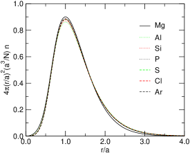
Figure 1: (color online) The scaled radial probability distribution for the valence electrons of the second row atoms Mg through Ar, as a function of distance in units of the radius $a$ of peak radial density.

The atom radius $a$ is plotted in Fig 2(a) versus valence number $N$; it gradually decreases as the number of particles increases, indicating a rapidly increasing density. A least squares fit to the Slater shielding model [Eq. (20)] with $n^{2}\!=\!9$ for the 2nd row atoms yields an excellent fit to $a$ with shielding constants $A\!=\!2.350(22)$ and $B\!=\!0.611(4)$. This corresponds to a 75% effective shielding of the nucleus from electrons in the 3(s,p) shells by each electron in the 2(s,p) shells and 39% shielding by each of the other $\rm 3(s,p)$ electrons in the Slater model, close to Slater’s rule of thumb values of 85% and 35%.

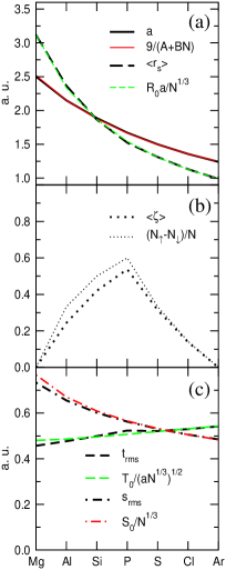
Figure 2: (color online) Density functional parameters as function of valence-electron number $N$. Part (a) shows the radius of peak radial density $a$ and the system-averaged Wigner-Seitz radius $\langle r_{s}\rangle$, (b) shows the system-averaged spin polarization $\langle\zeta\rangle$ as compared to the fractional difference in occupation number $(N_{\uparrow}-N_{\downarrow})/N$ for each spin, (c) shows the system-averaged inhomogeneity parameters $\langle t^{2}\rangle$ and $\langle s^{2}\rangle$ as compared to scaling predictions.

Also shown in Fig 2 are system averages [Eq. (16)] of the parameters used in characterizing the semilocal density functional theory of the exchange-correlation hole. Fig 2(a) shows the system-averaged Wigner-Seitz radius $\langle r_{s}\rangle$. This decreases with $N$ more rapidly than the atom radius $a$, varying from 3 to roughly 0.9 as one goes from Mg to Ar. This reflects the two simultaneous effects of an increasing number of electrons and a shrinking atomic radius as one crosses the row.

The average polarization $\langle\zeta\rangle$ shown in Fig 2(b) ranges between zero for the closed shell systems Mg and Ar, and a maximum value near 0.6 for P, at half-filling of the 3p shell, and varies smoothly in between. Although $\zeta$ is defined locally [Eq. (13)], its system average approaches the natural global measure, $\left(N\uparrow-N\downarrow\right)/N$, also shown in Fig 2(b). It might do this better if anisotropic densities were used in its system average.

The inhomogeneity factor $s_{rms}\!=\!\sqrt{\langle s^{2}\rangle}$ for the exchange hole and $t_{rms}\!=\!\sqrt{\langle t^{2}\rangle}$ for the correlation hole are shown in Fig 2(c). They show, as expected, somewhat different scaling behavior, with $s_{rms}$ decreasing with system size and $t_{rms}$ fairly constant. The values indicate systems with a moderate degree of inhomogeneity. As one might expect, an isolated atom on average lies outside of the perturbative limit $s^{2}<0.3$ characteristic of solids, but does not quite reach the threshold of severe inhomogeneity, $s^{2}\!=\!1$, across the entire system.

Best-fit global scaled parameters $\tilde{r}_{s}$, $\sqrt{\tilde{s}^{2}}$ and $\sqrt{\tilde{t}^{2}}$ [Eqs. (23,25,26)] are also shown in Fig. 2. The fits are weighted towards the high-$N$ end of the row, which shows almost perfect scaling behavior. There is excellent agreement between the actual trend of $\langle r_{s}\rangle$ and that predicted by scaling, with $R_{0}\!=\!1.592(15)$. There is also quite good agreement between the scaling form for $\langle s^{2}\rangle$ and the observed value, with a falloff in quality at small $N$ because the gradient of the density does not scale as cleanly with $N$ as does the density. The value of $\langle t^{2}\rangle$ shows additional behavior that follows the spin polarization. This is absent if the system-average is taken over the density of antiparallel-spin particle pairs rather than the total pair density. Scaling values for these parameters are $S_{0}\!=\!0.969$ and $T_{0}\!=\!0.856$.

IV.3 Exchange and correlation holes

Shown in Fig. 3(a) are system-averaged exact exchange holes evaluated numerically from Eqs. (8) and (9) and DFT models of the same, for three atoms: Mg with a filled 3s shell, P with a half-filled 3p shell, and Ar with a closed 3p shell. The data for P and Mg have been shifted downward slightly for clarity. Each curve is weighted by factor of $2\pi u$ so that its integral gives the potential energy per particle associated with the hole. It thus shows where the most significant contributions to the overall energy come from. The holes are scaled by a factor $\langle r_{s}\rangle^{3}/N$ and plotted versus the scaled interparticle distance $\langle r_{s}\rangle$ to reflect the scaling Perdew and Wang (1992) of a non-polarized exchange hole under uniform scaling of the density. The trends for the atoms not shown are quite similar.

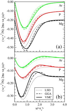
Figure 3: (color online) Scaled and weighted system-averaged exchange hole (a), and correlation hole (b), plotted versus scaled distance $u/\langle r_{s}\rangle$ for Mg, P, and Ar. VMC data are solid, the LSD model are dotted and the PBE GGA are dashed lines. Curves for P and Mg are shifted downward for clarity; in reality they tend to zero for small and large $u$.

In comparison, the LSD hole Perdew and Wang (1992) is excellent for small $u$, out to around the maximum of the main “dip” that contributes the most to the exchange energy. At the same time this main feature is too narrow in width. The portion of the hole missing is spread out into a long range tail that reflects the abrupt cutoff in occupation of states at the fermi wavevector in a homogeneous electron gas. This tail contains a noticeable proportion of the total particle sum-rule of the exchange hole (calculated by weighting the hole by $4\pi u^{2}$) but because of a negligible contribution (weighted by $2\pi u$) to the exchange energy, causes it to be underestimated.

The GGA hole, designed to reproduce the PBE exchange energy Ernzerhof and Perdew (1998), improves upon the LSD by truncating the long-range tail and collecting this portion of the LSD hole to form a broader hole at its minimum. While failing to capture exact details, it mimics quite nicely on average what happens in the exact exchange hole, and thus leads upon integration to a much improved exchange energy. Interestingly, the GGA is slightly less accurate than the LSD in the short-$u$ range of the hole, where presumably the gradient expansion upon which the GGA is based should be most accurate.

The LSD quite faithfully scales with $\langle r_{s}\rangle$ – for example, the position of the minimum in the curve is the same for all three atoms. The numerical result for the exact hole agrees with the LSD for Ar but is shifted to larger $u$ for Mg. The GGA only partly follows suit. The reasons for this shift will become clear in Section IV.5.

Figure 3(b) shows the energy-weighted correlation hole for three cases of Mg, P, and Ar. The hole data and interparticle distances are scaled and shifted in the same fashion as the exchange hole data. The plot shows VMC data as a thick solid line, as well as the predictions of the LSD and the PBE GGA model Perdew et al. (1996).

The correlation holes consist of a short-range region where the density of electron pairs is reduced and a region at longer distances where it is enhanced; an overall sum rule of zero is required. The length scale of the hole roughly follows $\langle r_{s}\rangle$, increasing as the number of particles decreases. The overall hole has a well defined finite range, with the density removed at short range collected into a noticeable “bump” with a maximum at a distance between 1.33 and 2 times that of the valence shell radius $a$. This is intuitively reasonable since there is little physical reason to enhance the pair density at interelectron distances much larger than the diameter of the atom. The shape of the hole varies noticeably from more compact to more spread out as one moves across the periodic table. Likewise, the strength of the correlation hole relative to the exchange hole varies considerably, with the relative strength of the Mg hole more than twice that of Ar. This follows the trend in the homogeneous electron gas from highly correlated to uncorrelated behavior as $r_{s}$ decreases  Ortiz and Ballone (1994). Unlike exchange, where the particle sum-rule enforces more or less the same size hole in units of $r_{s}$, the zero sum-rule of correlation places little constraint on the size of the hole.

As with exchange, the LSD hole tends to predict the short range shape of the hole quite well, with a disagreement in the on-top ($u\!=\!0$) hole of 10$\%$ hidden by the $2\pi u$ weighting. The hole tends to be too deep and too wide. The major disagreement is at long distances: the HEG model for correlation includes a long-ranged tail that screens out the long-ranged behavior in exchange. To compound the effect, the system-average hole at long distances is dominated by contributions from the low-density asymptotic region of the atom. These in the LSD approximation generate unrealistically long tails to the system average. The LSD hole for an atom ends up predicting that the electron pair density removed at short range is redistributed out to infinity at a rate that surprisingly decays even more slowly than in the HEG.

The GGA model includes gradient corrections at short range, given by a gradient expansion of the HEG model. These lift up the correlation hole at short and intermediate distances, creating a markedly better match to the VMC results, especially for Ar. The zero sum rule for correlation is imposed by a finite-range cutoff of the correlation hole, which has the added benefit of killing the long-range tails of the LSD hole. One therefore finds a consistent, systematic improvement on the LSD. However the GGA hole dies out too slowly as compared to the VMC at long range, so that the positive peak is too spread out and contributes less to the energy integral than in the VMC case. It is thus easier than in the case of exchange to detect the systematic error in the PBE model – an overestimate of the size of the correlation energy.

IV.4 Exchange-correlation energy

Fig. 4 shows correlation, exchange, and exchange-correlation energies for our VMC data, and for the LSD and PBE density functional models. The VMC data is taken from integrating numerically the associated holes using Eq. 5 restricted to $\lambda\!=\!0$ for exchange and $\lambda\!=\!1$ for exchange-correlation. The density functional values are evaluated directly from the VMC density using the energy-per-particle definition conventional for DFT applications Jones and Gunnarsson (1989); PBE . The energies are scaled by the exchange scaling factor of Eq. (27), appropriate, within the LSD approximation, for a density which uniformly scales as a function of particle number $N$. This produces a nearly constant scaled value for the exchange energy in the LSD, indicating the validity of the underlying picture. The scaled exchange energy $\bar{E}_{x}^{LSD}\!=\!-0.390(2)$ hartree may be compared to the homogeneous electron gas value of -0.4582 hartree, a reasonable agreement considering the arbitrariness inherent in the definitions [Eq. (16)] of $\langle r_{s}\rangle$ and $\langle\zeta\rangle$. The spin scaling of the correlation energy is not the same as for exchange, as demonstrated by a “bump” at half-filling that correlates positively with $\langle\zeta\rangle$.

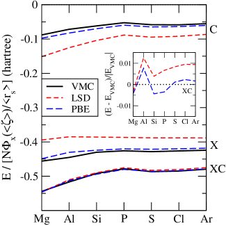
Figure 4: (color online) Exchange, correlation and exchange-correlation potential energy per particle for the valence shell of second row atoms, scaled by the factor $N\phi_{x}(\langle\zeta\rangle/\langle r_{s}\rangle)$ as described in text. Thick solid line is VMC data; short-dashed and long-dashed lines are LSD and GGA predictions. Energy in atomic units. Inset: relative differences between the two DFT models and the VMC data for the exchange-correlation energy.

Fig. 4 demonstrates the dramatic cancellation of errors in the exchange and correlation components in the LSD. The LSD underestimates the effect of exchange, having too much of the sum-rule of the hole in its long-range tail, and overestimates the resulting screening of this long-range tail in correlation. The overall error in the exchange-correlation energy, however, is a full order of magnitude smaller than that of either exchange or correlation alone. Having a hole derived from an accurate many-body calculation of a true electronic system pays off in physically driven error cancellation. The PBE GGA implements a consistent correction of these two effects, by simultaneously creating a more compact exchange hole and cutting off the correlation hole at long range. It recovers the bulk of the errors in the LSD for exchange and correlation separately. The averaged difference per electron between numerical exchange energies or VMC-simulated correlation energies and their DFT counterparts are shown in Table 2. The improvement from LSD to PBE is an order of magnitude for both exchange and correlation but more modest for the two combined.

The major source of error in our calculation of the exact exchange energy is from the numerical integration of the exchange hole, giving errors typically less than one part in $10^{5}$ for the grid used, and is negligible here. The VMC results for correlation should in principle be a variational upper bound, assuming no numerical error in extracting them from pair density data and the numerical calculation of exchange. The true correlation energy, being lower in energy, should be closer to the DFT predictions. To estimate this error in the VMC, one can compare the roughly three millihartree error of our total VMC energy for Si (Table 1), which we can attribute to an incomplete treatment of correlation, with a 20 millihartree difference between VMC and PBE correlation energies for Si. On the other hand, the VMC is potentially exact for the nodeless Mg valence shell – the variational wavefunction used converges to the exact one – here the PBE has a 10 millihartree error with respect to the VMC, recovering 50% of the error in the LSD.

Table 2: Mean absolute relative differences (mard) and mean absolute difference per electron (mad), in millihartrees, between DFT models and numerical data for exchange (X) , correlation (C) and exchange-correlation (XC) potential energies.

	X		C		XC
	LSD	PBE	LSD	PBE	LSD	PBE
mard	0.105	0.017	0.657	0.117	0.0076	0.0035
mad	28.4	4.7	26.0	4.6	2.6	1.0

The relative difference between VMC and DFT exchange-correlation energies is shown in the inset of Fig. 4. It is basically on the order of the expected variational bias, with a mean signed relative difference of less than 0.01%. A expected downwards shift of 5% in correlation energy due to variational bias will cause a much smaller relative change in the XC energy, given that correlation is a small fraction of this energy. The shift is 0.5% in the case of Ar; those for smaller $N$ should be similar, involving smaller variational biases but larger relative correlation energies. Overall, then, the PBE XC energy may be roughly 0.5% higher than that of the exact ground-state, but systematically removing most of the LSD error.

One may take the exchange scaling analysis one step further to analyze the gradient contributions to the exchange and correlation energies. In particular, the GGA predicts a multiplicative correction to the LSD exchange energy-per-particle of

$$\epsilon_{x}^{GGA}/\epsilon_{x}^{LSD}\sim 1+\mu s^{2},$$ (39)

for small values of $s^{2}$. The PBE data in Fig. 4 shows a slight variation from LSD scaling for smaller $N$ or larger $\tilde{s}^{2}$ which can be fit to Eq. (39). The value of $\mu$ thus obtained is $0.351$ for the GGA data as compared to $0.431$ for the exact calculated exchange, a 20% stronger response to inhomogeneity than the GGA prediction.

IV.5 Scaling trends of exchange and correlation holes

Under a uniform scaling of the density – and constant particle number $N$ – the exchange hole is invariant. As our densities scale fairly uniformly, but with $N\!=\!Z$ not constant, it is informative to see what extent the exchange hole can be reduced to a scaling form. This is most easily done by considering the spin-decomposed exchange hole, Eq. (8). To do so, we use an identifiable point of each hole – the minimum of the energy-weighted hole – to determine a length scale $r_{X}^{\sigma}$ for each spin species $\sigma$. The hole is normalized by the number of particles of that spin to guarantee a sum rule of -1. Uniform scaling then entails the same procedure as for the radial probability density: $n_{x}^{\sigma}$ scales to $(r_{X}^{\sigma})^{3}n_{x}^{\sigma}$ as distance is scaled from $u$ to $u/r_{X}^{\sigma}$. The results are shown in Fig. 5.

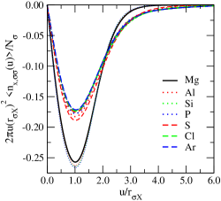
Figure 5: (color online) Scaled minority-spin (thinner lines) and majority-spin (thicker lines) exchange holes for second row pseudopotential atoms plotted versus a spin-dependent, scaled interparticle distance $u/r_{X}^{\sigma}$. Each hole is scaled by $(r_{X}^{\sigma})^{3}$ and weighted by $2\pi$ times the scaled interparticle distance. The scaling length $r_{X}^{\sigma}$ is determined by the distance at which the weighted hole has its minimum value.

We do see scaling behavior, but interestingly, two scaling forms. There is a striking difference between the hole formed from a single particle, (in Mg, and the minority spin channel of Al through P) and that of two or more particles. The two cases that disagree slightly from this trend are, quite naturally, the two cases with only two electrons in a given spin channel, Al and Si. Otherwise the results neatly scale on top of each other.

This result is not that surprising if we consider the form of the exchange hole in Eq. (8). For one particle in a given spin, the form reduces to a convolution of the spin density $n_{\sigma}({\bf r})\!=\!|\psi_{3s}^{\sigma}({\bf r})|^{2}$ and leads to a relatively compact function. The hole merely removes the self-interaction error of the Hartree approximation, and in a sense is not a true exchange hole. The $N_{\sigma}\!>\!1$ case also includes convolutions of the overlap of two different orbitals $\psi^{*}_{i,\sigma}({\bf r})\psi_{j,\sigma}({\bf r})$, that describe the exchange of two electrons. Such overlap terms are naturally more spread out than a single-orbital probability and create a more slowly decaying hole. Note that the exchange scaling law [Eq. (21)] requires that both forms scale uniformly with an isolectronic (fixed $N$) uniform scaling of the density, but with significantly different asymptotic forms because of their different origins. Finally it is interesting to note how quickly the transition from the self-interaction dominated to an exchange dominated hole occurs – the large number limit is essentially reached starting at $N_{\sigma}\!=\!2$.

Fig. 6 shows scaling lengths for the majority (up) spin and minority (down) spin exchange holes, $r_{X}^{\uparrow}$ and $r_{X}^{\downarrow}$, in units of the valence-shell radius $a$ for each atom in the second row. In addition, the average Wigner-Seitz radius $\langle r_{s}\rangle$ is plotted and the equivalent spin-dependent radii $\langle r_{s}^{\sigma}\rangle=\langle r_{s}\rangle(1+\sigma\zeta)^{-1/3}$, proportional to the natural length-scale $(k_{F}^{\sigma})^{-1}$ of the spin-decomposed LSD exchange hole. These are scaled by a factor of 0.755 so that they match $r^{\sigma}_{X}$ for Ar. The comparison between the actual length-scales $r_{X}$ and the LSD equivalent shows the separation of the single-particle and multi-particle cases seen in Fig. 5. For spin occupation $N_{\sigma}>1$, the $r_{X}$ values are well predicted by LSD theory. For $N_{\sigma}\!=\!1$ the hole scales as $a$, and is notably larger than the LSD prediction. In this case, the length scale is set simply by the width $\sim a$ of the single orbital occupied.

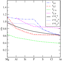
Figure 6: (color online) Various scaling lengths discussed in the paper. Shown versus valence electron number are: the position of maximum depth ($r_{X}$) in the spin-up (red) and spin-down (blue) energy-weighted exchange holes, the same ($r_{C}$) for antiparallel (green) and parallel spin correlation holes, all scaled by the effective valence bohr radius $a$. System-averaged Wigner-Seitz radius $\langle r_{s}\rangle$ for the total density (black) and each spin density (dotted lines) are also shown, scaled by a factor of $c\!=\!0.755$ to aid in comparison.

Unlike exchange, the universal scaling law for correlation [Eq. (29)] is nontrivial, and the correlation energy and hole are nontrivial to model even for the homogeneous electron gas. Nevertheless, Fig. 3(b) shows that correlation holes for the second row atoms are qualitatively similar and it is instructive to scale the holes to highlight the trends that occur as one crosses the row.

To do this we use an empirical scaling relation that matches the holes as closely as we find possible. It is again helpful to spin-decompose the holes, into antiparallel-spin (A) and parallel-spin (P) channels. A scaled form $\bar{n}_{c}(x)$ of the hole in either channel may be constructed as

$$2\pi u\langle n_{c}^{A,P}(u)\rangle=2\pi(u/r^{A,P}_{C})N_{A,P}\;\bar{n}_{c}^{A,P}(u/r^{A,P}_{C}),$$ (40)

where $N_{A}$ and $N_{P}$ are the number of electron pairs of either spin channel and $r^{A}_{C}$ and $r^{P}_{C}$ are scaling lengths. These are again chosen as the distance at which the energy-weighted holes take their minimum value. This optimizes the match between holes at short interparticle distances at the expense of that at longer ones. The results are shown as a function of scaled interparticle distance in Fig. 7; scaling lengths are shown in Fig. 6.

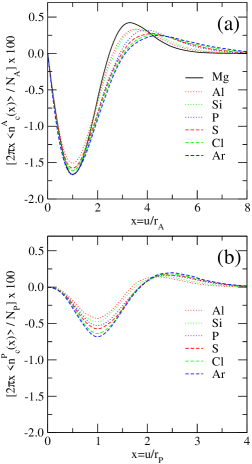
Figure 7: (color online) Scaled correlation holes for second row pseudopotential atoms. Part (a) shows the correlation hole at full coupling for antiparallel-spin electrons, weighted by $2\pi$ times the interelectron distance $u$. The holes are scaled by the number of antiparallel electron pairs $N_{A}$ and plotted versus the scaled electron distance $x=u/r^{A}$, where $r^{A}$ is the distance at which each weighted hole has a minimum. Part (b) shows the analog for the parallel-spin correlation hole, in terms of parallel-spin pair number, $N_{P}$ and scaling radius $r^{P}_{C}$. Each hole is plotted in atomic units.

For the case of antiparallel-spin electron pairs [Fig. 7(a)], the results at short distances match up closely. The minimum of the holes shows some shell structure, with the closed spin-shell atoms Mg, P and Ar with the deepest holes. At long range, there is a systematic trend as the $3p$-shell is filled, going from a compact hole with a sharp positive peak, to a relatively wider hole with a positive peak spread out over a large range of distance relative to $r^{A}_{C}$. The trend seems to be one of gradual reduction of finite-size effects at long-range, with the shape of the hole trending to that of the homogeneous electron gas, with its infinite-ranged hole.

The parallel-spin holes are shown in Fig. 7(b). That for Mg is trivially zero since there are no same-spin pairs. As shown in Fig. 6, $r^{P}_{C}$ is almost exactly twice that of $r^{A}_{C}$ across the second row so that each subplot of Fig. 7 shows the same physical range in distance for each atom despite the different abscissas. The hole-per-pair is significantly smaller than in the antiparallel spin channel and is concentrated at longer interparticle distance. Both effects are caused by the exchange hole which removes most of the probability of finding particles of the same spin at short range. As one goes across the shell, the tendency is for gradually deeper and longer-ranged holes. Finally, given the equivalence $r^{P}_{C}\!=\!2r^{A}_{C}$, one finds that the scaled antiparallel and parallel holes-per-pair for each atom match fairly closely at large distances ($r^{A}_{C}\!>\!5$). At distances longer than the effective exchange hole radius, it seems that electrons no longer detect each other’s spins.

All-electron spherically-averaged Coulomb hole data for nearly spherical molecules and atoms show qualitatively very similar results to ours, after taking into account the $4\pi r^{2}$ weighting typically used in the literature Banyard and Mobbs (1981); Wang et al. (1994); Gálvez et al. (2005); *Galvez:044319; Toulouse et al. (2007). The hole at small interparticle distances typically shows the evidence of shell and molecular structure, but significantly reduced by the effects of system averaging, particularly in the large-$Z$ limit. The qualitative shape of the peak at large interparticle distances seems to be a universal feature of the Coulomb/correlation hole and closely matches the behavior seen in Figs. 3(b) and 7. Shell analysis of the hole for small atoms Banyard and Mobbs (1981) tells us that this feature is caused by electrons in the valence shell and is thus apropos for comparison to our data. Using the point of crossover $r_{cr}$ from negative hole to positive peak as a point of reference, we find that our scaling model provides a fairly good prediction for other data. A fit of this point to our data yields $r_{cr}=1.5*R_{0}a/N^{1/3}$ for Si; using this formula and the naive Slater model for $a$ we predict Coulomb hole crossover points for the C isolectronic series that range from 11.2 a.u. for C to 8.3 a.u. for Ne⁺⁴, which are indistinguishable from those of the Coulomb hole plots of VMC data for the series Gálvez et al. (2005); *Galvez:044319. This suggests that our data may be useful to analyze the long-range trends of correlation holes of atoms and small molecules.

A few extra notes are in order – first of all, the point of comparison between holes found to be most successful is the correlation hole per pair and not per particle, as with exchange. A particle number for the antiparallel-spin hole cannot be unambiguously defined, and we find no scheme for a per-particle hole that provides as consistent a scaling fit for the series. At the same time, the scaled hole used here is not scale-invariant, in which case the hole, having units of volume, should scale as $1/r_{scale}^{3}$. It is therefore not unitless, but rather varies as $1/a_{0}^{2}$ given the choice of atomic units. The situation is reminiscent of that of the slowly varying electron gas, in which the inhomogeneity in the exchange hole can be described by the scale-invariant parameter $s$, but the correlation hole depends on the non-scale-invariant $t\sim s/\sqrt{r_{s}}$. However, it is not impossible to scale the correlation hole with a uniform scaling hypothesis of the form:

$$\langle n_{c}(u)\rangle=\frac{F(N_{\uparrow},N_{\downarrow})}{(r_{scale})^{3}}\bar{n}_{c}(u/r_{scale})$$ (41)

for an arbitrary function $F(N_{\uparrow},N_{\downarrow})$ of the number of valence electrons of each spin. In this case, the absence of scaling behavior is assumed to lie in the arbitrary amplitude $F$. The two approaches may be considered equivalent since the normalization used in Eq. (40) is implicitly a function of $N_{\uparrow}$ and $N_{\downarrow}$.

It is also worth noting that length-scales for correlation and exchange diminish as a proportion of atom radius $a$ in going from Mg to Ar (Fig. 6). Finite size effects in exchange and correlation become important as $\langle r_{s}\rangle/a$ approaches unity – that is, the length-scale of the XC hole approaches the system size of the atom. We thus expect, and find, the largest errors for local DFT’s for Mg, for which $\langle r_{s}\rangle/a$ is largest, and the smallest for Ar. Nevertheless, the GGA parameter $t^{2}$ used to estimate this inhomogeneity error has a system average that increases as one proceeds down the row. In the slowly varying electron gas, the higher the electron density, the more sensitive correlation is to inhomogeneity, but in atoms, the higher the density, the less effect the finite size of the atom has on correlation. This misidentification is a natural limitation of using a semilocal parameter to measure the effect of inhomogeneity, which for atoms as essentially zero-dimensional objects must necessarily depend on global features. Interestingly, however, the PBE correlation hole does take into account one global measure, the zero particle-sum-rule of the hole. For very inhomogeneous systems, this constrains the hole to react more strongly at larger $r_{s}$ to a given value of $t^{2}$. Thus it follows to a fair degree the observed finite-size effects, more so than one might have expected.

IV.6 Pair correlation function

One can gain more insight into the behavior of correlation with atomic number, and in particular the role of finite size effects, by calculating a pair correlation function $g_{c}$, defined as the ratio of the pair density of the fully correlated ($\lambda\!=\!1$) system to that of the equivalent noninteracting system ($\lambda\!=\!0$):

$$g_{c}(u)=\frac{\langle n^{(2)}_{\lambda=1}(u)\rangle}{\langle n^{(2)}_{\lambda=0}(u)\rangle}.$$ (42)

This maps the fractional change, because of Coulomb correlation, in the expected number of particle pairs as a function of distance. As the noninteracting-system pair density already incorporates exchange, this measures a purely correlation effect, and is somewhat different from the normal definition of $g$ measured relative to the pair density of independent particles. The value at zero separation, $g_{c}(0)$, measures the on-top hole for antiparallel spin correlation. Because of fermi statistics, the parallel-spin channel contributes zero to both numerator and denominator of the on-top value of Eq. (42).

We show the VMC values for $g_{c}(u)$ for the second row atoms in Fig. 8. As a comparison, the equivalent system-averaged on-top pair correlation function for the LSD, $\langle g^{LSD}_{c}(0)\rangle$, calculated by the same system-averaging technique as Eq. (16), is shown as circles at $u\!=\!0$. At short range the pattern of the VMC data is similar to the correlation hole in the HEG Ortiz and Ballone (1994) except for deviations, due to small-number statistics, from an expected cusp Kimball (1973) at very short interparticle distances. Given the noise in the VMC in this region, the LSD and VMC values for the on-top hole are in reasonable agreement. At long range one sees a marked enhancement of the distribution of particle pairs relative to the uncorrelated pair density. The long-range asymptotic value of the pair distribution function in the HEG is one, indicating a vanishing difference between correlated and uncorrelated distributions. In atoms, this is not a requirement, and in fact the enhancement of pairs at long range is surprisingly large for Mg. The distances in this case are bigger than the distance from the peak of the valence density on one side of the atom to that on the other, about 1.7 $a$ or roughly 3.5 a.u. for Mg. There is a large fractional enhancement of the relatively small density of pairs separated by several atomic radii, in contrast to the modest enhancement of the long-range pair density for more localized holes. This is consistent with an “in-out” correlation where if one electron is found on the inside of the valence shell the other is favored to be found on the outside edge of the shell.

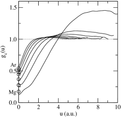
Figure 8: The correlation contribution to the pair correlation function, $g_{c}$, for the valence shell of the second row atoms plotted versus interparticle distance $u$. The curve for Ar and Mg are labelled at $u\!=\!0$. Also shown (circles) is the system-averaged on-top or $u\!=\!0$ pair-correlation function for the LSD.

V Discussion

The valence shell of first or second row atoms, within the pseudopotential approach, is an example of uniform scaling that has been known from the earliest stages of atomic physics. The form of scaling is related to that of the Thomas-Fermi scaling of the all-electron density for large atoms, in that the net charge of the system is kept fixed as the system is scaled, and so scaling parameters such as $\langle r_{s}\rangle$ depend upon the number of electrons $N$. It differs in that the scaling parameter $a$ does not have a simple power-law behavior with $N$, but essentially a Pade-like dependence, as noted by Slater, because of the role of self-interaction. At the same time, the scaling of a single shell is a form of uniform scaling to high density, and might be a useful complement to the standard example of isoelectronic scaling. What happens in the current case, in the limit of a very large-degeneracy shell, for which $N\gg 1$ is achievable?

Intriguingly, the exchange hole has not one, but two, scaling forms – with the single-orbital hole fundamentally different from those that are constructed with two or more orbitals. Self-interaction effects spoil the invariance of the exchange hole under uniform scaling with constant net charge that would hold with constant particle number. But at the same time, self-interaction effects die out astonishingly rapidly, with systems of three or more electrons already showing large-$N$ scaling behavior. Correlation holes do not scale uniformly and trends across the second row cannot be unambiguously modeled. Nevertheless, a clear trend with the scaling of the density does occur: the transition from more correlated, low density systems in which finite size effects dominate the correlation peak at large interparticle distances, to higher density ones in which the system-averaged hole approaches that of the HEG, and the GGA approximation is very good. The natural parameter to characterize this trend, the ratio $\langle r_{s}\rangle/a$ of average hole radius to atomic radius, can not be modeled in a semilocal DFT, but the use of a different constraint – a cutoff based on the correlation hole sum rule – does a reasonable job of following it. The qualitative behavior of the positive correlation peak is seen in all-electron calculations and a crude estimate indicates that scaling results for this feature should apply to atoms and spherical molecules in general.

It is of interest to analyze the sources of error in the PBE correlation hole by decomposing the system averaging. The PBE hole near the valence peak determines the overall shape of the system-averaged hole but, since gradients are small in this region, has an unphysical long-range tail equivalent to that of the LSD hole. Holes in the pseudopotential core and far from the atom deviate dramatically from the system average but cut off just at the right length scale. They end up contributing the most to the positive peak of the system-average that, physically, is caused by finite size of the atom. It is not the local XC hole but its system-average that the PBE is capturing, as it was designed to do.

Our data thus show that for the type of system studied here, the semilocal PBE GGA model works essentially as advertised. The significant defects of the XC hole in the LSD approach are more or less fixed, especially for the crucial aspect of the hole – the integral that produces the exchange and correlation energy. The reason for this success is likely related to the simplicity of the single-shell structure studied, with the main physics being scaling behavior similar to that which the PBE was built to represent. The main source of error, the poor treatment of finite-size effects, occurs mainly in the long-range tail of the GGA XC hole which does not contribute much to the total energy.

The PBE does somewhat underestimate the gradient correction parameter $\mu$ [Eq. (39)] needed for valence-shell exchange energies. Recent work on modifying the PBE for solids Armiento and Mattsson (2005); Perdew et al. (2008); Zhao and Truhlar (2008) indicates that use of a value for $\mu$ half that of the PBE, but consistent with the gradient expansion for a slowly-varying electron gas, leads to improved lattice constants and bulk moduli (if poorer cohesive energies). The PBE choice, is instead best suited for predicting total energies of atoms and binding energies of molecules. Our work thus emphasizes the incompatibility between GGA’s designed for molecules and those for solids. The large value of $\mu$ needed for total atomic energies has been attributed Perdew et al. (2006) to using the gradient correction to account for exchange energy corrections caused by the cusp in electron density near the nucleus. This is should not be true in the present case since the nucleus has been replaced by a smooth pseudopotential. It seems that another mechanism is at play here, quite possibly self interaction. The PBE models systems with large self interaction error, like the two-electron valence shell of Mg, very well. But this is perhaps at a cost of overcorrecting in situations like the slowly varying electron gas where inhomogeneity and not self-interaction is the predominant issue. Another consideration is the boundary condition difference between finite and infinite systems, with the former needing a stronger correction to produce a more sharply defined long-range cutoff to the hole.

Our work also points to the difficulty of imposing a self-interaction correction to the GGA. To the extent that the GGA may be correcting LSD error caused by self-interaction and not by the imperfect treatment of inhomogeneity, applying a self-interaction correction to the GGA would lead to correcting the same problem twice. Any self-interaction correction based on a GGA would require a remarkable degree of cancellation of errors between the correction for exchange and that for correlation to improve total energies for the systems studied here. The exploration of self-interaction corrected GGA models that could have this level of error cancellation might thus be of interest.

VI Acknowledgments

One of us (ACC) thanks John Perdew and Cyrus Umrigar for helpful discussions and comments.

References

- Hohenberg and Kohn (1964) P. Hohenberg and W. Kohn, Phys. Rev. 136, B864 (1964).
- Jones and Gunnarsson (1989) R. O. Jones and O. Gunnarsson, Rev. Mod. Phys. 61, 689 (1989).
- Levy and Perdew (1985) M. Levy and J. P. Perdew, Phys. Rev. A 32, 2010 (1985).
- Levy (1991) M. Levy, Phys. Rev. A 43, 4637 (1991).
- (5) J. Harris and R. O. Jones, J. Phys. F: Met. Phys. 4, 1170 (1974); D. C. Langreth and J. P. Perdew, Solid State Commun. 17, 1425 (1975); O. Gunnarson and B. I. Lundqvist, Phys. Rev. B 13, 4274 (1976).
- Scott (1952) J. M. C. Scott, Philosophical Magazine Series 7 43, 859 (1952).
- March (1957) N. H. March, Advances in Physics 6, 1 (1957).
- Perdew et al. (2006) J. P. Perdew, L. A. Constantin, E. Sagvolden, and K. Burke, Phys. Rev. Lett. 97, 223002 (2006).
- Perdew et al. (2008) J. P. Perdew, A. Ruzsinszky, G. I. Csonka, O. A. Vydrov, G. E. Scuseria, L. A. Constantin, X. Zhou, and K. Burke, Phys. Rev. Lett. 100, 136406 (2008).
- Perdew et al. (2009) J. P. Perdew, A. Ruzsinszky, G. I. Csonka, L. A. Constantin, and J. Sun, Phys. Rev. Lett. 103, 026403 (2009).
- Perdew (1991) J. P. Perdew, in Electronic Structure of Solids ’91, edited by P.Ziesche and H.Eschrig (Akademie Verlag, Berlin, 1991).
- Perdew et al. (1996) J. P. Perdew, K. Burke, and Y. Wang, Phys. Rev. B 54, 16533 (1996).
- (13) J. P. Perdew, K. Burke, and M. Ernzerhof, Phys. Rev. Lett. 77, 3865 (1996); 78, 1396(E) (1997).
- Becke (1993) A. D. Becke, J. Chem. Phys. 98, 5648 (1993).
- Constantin et al. (2006) L. A. Constantin, J. P. Perdew, and J. Tao, Phys. Rev. B 73, 205104 (2006).
- Coulson and Neilson (1961) C. A. Coulson and A. H. Neilson, Proc. Phys. Soc. 78, 831 (1961).
- Koga and Matsuyama (1997) T. Koga and H. Matsuyama, J. Chem. Phys. 107, 8510 (1997).
- Matsuyama et al. (1998) H. Matsuyama, T. Koga, E. Romera, and J. S. Dehesa, Phys. Rev. A 57, 1759 (1998).
- Koga (2000) T. Koga, J. Chem. Phys. 112, 6966 (2000).
- Banyard and Mobbs (1981) K. E. Banyard and R. J. Mobbs, J. Chem. Phys. 75, 3433 (1981).
- Fradera et al. (2000a) X. Fradera, M. Duran, and J. Mestres, J. Chem. Phys. 113, 2530 (2000a).
- Fradera et al. (2000b) X. Fradera, M. Duran, R. Valderrama, and J. M. Ugalde, Phys. Rev. A 62, 034502/1 (2000b).
- Wang et al. (1992) J. Wang, A. N. Tripathi, and V. H. Smith, J. Chem. Phys. 97, 9188 (1992).
- Wang et al. (1994) J. Wang, A. N. Tripathi, and V. H. Smith, J. Chem. Phys. 101, 4842 (1994).
- Cioslowski and Liu (1998) J. Cioslowski and G. Liu, J. Chem. Phys. 109, 8225 (1998).
- Cioslowski and Liu (1999) J. Cioslowski and G. Liu, J. Chem. Phys. 110, 1882 (1999).
- Cancio et al. (2000) A. C. Cancio, C. Y. Fong, and J. S. Nelson, Phys. Rev. A 62, 062507 (2000).
- Gálvez et al. (2005) F. J. Gálvez, E. Buendía, and A. Sarsa, J. Chem. Phys. 123, 034302 (2005).
- Gálvez et al. (2006) F. J. Gálvez, E. Buendía, and A. Sarsa, J. Chem. Phys. 124, 044319 (2006).
- Toulouse et al. (2007) J. Toulouse, R. Assaraf, and C. J. Umrigar, J. Chem. Phys. 126, 244112 (2007).
- Thakkar et al. (1984) A. J. Thakkar, A. N. Tripathi, and V. H. Smith, Int. J. Quantum Chem. 26, 157 (1984).
- Gori-Giorgi and Savin (2005) P. Gori-Giorgi and A. Savin, Phys. Rev. A 71, 032513 (2005).
- Nagy (2006) A. Nagy, J. Chem. Phys. 125, 184104 (2006).
- Buijse and Baerends (1995) M. A. Buijse and E. J. Baerends, in Density Functional Theory of Molecules, Clusters and Solids, edited by D. E. Ellis (Kluwer Academic, Dordrecht, 1995).
- Fahy et al. (1990) S. Fahy, X. W. Wang, and S. G. Louie, Phys. Rev. Lett. 65, 1478 (1990).
- Hood et al. (1997) R. Q. Hood, M. Y. Chou, A. J. Williamson, G. Rajagopal, R. J. Needs, and W. M. C. Foulkes, Phys. Rev. Lett. 78, 3350 (1997).
- Hood et al. (1998) R. Q. Hood, M. Y. Chou, A. J. Williamson, G. Rajagopal, and R. J. Needs, Phys. Rev. B 57, 8972 (1998).
- (38) Maziar Nekovee, W. M. C. Foulkes, and R. J. Needs, Phys. Rev. Lett. 87, 036401 (2001); Phys. Rev. B 68, 235108 (2003).
- Cancio et al. (2001) A. C. Cancio, M. Y. Chou, and R. Q. Hood, Phys. Rev. B 64, 115112/1 (2001).
- Puzder et al. (2001) A. Puzder, M. Y. Chou, and R. Q. Hood, Phys. Rev. A 64, 022501/1 (2001).
- Hsing et al. (2006) C. R. Hsing, M. Y. Chou, and T. K. Lee, Phys. Rev. A 74, 032507/1 (2006).
- Slater (1930) J. C. Slater, Phys. Rev. 36, 57 (1930).
- Foulkes et al. (2001) W. M. C. Foulkes, L. Mitas, R. J. Needs, and G. Rajagopal, Rev. Mod. Phys. 73, 33 (2001).
- Kohn and Sham (1965) W. Kohn and L. J. Sham, Phys. Rev. 140, A1133 (1965).
- (45) It is of interest to note that the variation of the hole for a given physical system with coupling constant is equivalent to the uniform scaling of the density at fixed coupling constant. This would be a useful complement to the study we are carrying out.
- von Barth and Hedin (1972) U. von Barth and L. Hedin, J. Phys. C 5, 1629 (1972).
- Becke (1988) A. D. Becke, Phys. Rev. A 38, 3098 (1988).
- Lee et al. (1988) C. Lee, W. Yang, and R. G. Parr, Phys. Rev. B 37, 785 (1988).
- Armiento and Mattsson (2005) R. Armiento and A. E. Mattsson, Phys. Rev. B 72, 085108/1 (2005).
- Zhao and Truhlar (2008) Y. Zhao and D. G. Truhlar, J. Chem. Phys. 128, 184109 (2008).
- Becke (1998) A. D. Becke, J. Chem. Phys. 109, 2092 (1998).
- Tao et al. (2003) J. Tao, J. P. Perdew, V. N. Staroverov, and G. E. Scuseria, Phys. Rev. Lett. 91, 146401/1 (2003).
- Schmider and Becke (2000) H. L. Schmider and A. D. Becke, THEOCHEM 527, 51 (2000).
- Zhao and Truhlar (2006) Y. Zhao and D. G. Truhlar, J. Chem. Phys. 125, 194101 (2006).
- Perdew and Constantin (2007) J. P. Perdew and L. A. Constantin, Phys. Rev. B 75, 155109/1 (2007).
- Cancio and Chou (2006) A. C. Cancio and M. Y. Chou, Phys. Rev. B 74, 081202(R)/1 (2006).
- Ernzerhof and Perdew (1998) M. Ernzerhof and J. P. Perdew, J. Chem. Phys. 109, 3313 (1998).
- Perdew and Wang (1992) J. P. Perdew and Y. Wang, Phys. Rev. B 46, 12947 (1992).
- Burke et al. (1998) K. Burke, J. P. Perdew, and M. Ernzerhof, J. Chem. Phys. 109, 3760 (1998).
- (60) The presence of self-interaction error in the Hartree energy is what forces the constant term in this expression, and spoils a purely power-law behavior as seen in Thomas-Fermi scaling of the all-electron density.
- Oliver and Perdew (1979) G. L. Oliver and J. P. Perdew, Phys. Rev. A 20, 397 (1979).
- (62) The analogous relationship for the correlation hole is used to derive the scaling formula for the hole at full coupling [Eq. (17)].
- (63) D. R. Hamann, M. Schlüter, and C. Chiang, Phys. Rev. Lett. 43, 1494 (1979); G. B. Bachelet, D. R. Hamann, and M. Schlüter, Phys. Rev. B 26, 4199 (1982).
- Handy (1973) N. C. Handy, J. Chem. Phys. 58, 279 (1973).
- Schmidt and Moskowitz (1990) K. E. Schmidt and J. W. Moskowitz, J. Chem. Phys. 93, 4172 (1990).
- Kato (1957) T. Kato, Commun. Pure Appl. Math. 10, 151 (1957).
- Harrison and Handy (1985) R. J. Harrison and N. C. Handy, Chem. Phys. Lett. 113, 257 (1985).
- Filippi and Umrigar (1996) C. Filippi and C. J. Umrigar, J. Chem. Phys. 105, 213 (1996).
- Barnett et al. (2001) R. N. Barnett, Z. Sun, and W. A. Lester, J. Chem. Phys. 114, 2013 (2001).
- McMillan (1965) W. L. McMillan, Phys. Rev. 138, A442 (1965).
- Ceperley and Kalos (1979) D. Ceperley and M. H. Kalos, in Monte Carlo Methods in Statistical Physics, edited by K. Binder (Springer Verlag, Berlin, 1979).
- (72) S. Fahy, X. W. Wang, and S. G. Louie, Phys. Rev. Lett. 61, 1631 (1998); Phys. Rev. B 42, 3503 (1990-II).
- Mitáš et al. (1991) L. Mitáš, E. L. Shirley, and D. M. Ceperley, J. Chem. Phys. 95, 3467 (1991).
- Umrigar et al. (1988) C. J. Umrigar, K. G. Wilson, and J. W. Wilkins, Phys. Rev. Lett. 60, 1719 (1988).
- Kalos and Whitlock (1986) M. Kalos and P. Whitlock, Monte Carlo Methods, Vol. I (Wiley and Sons, New York, 1986).
- (76) D. Ceperley, Lecture notes.
- Ortiz and Ballone (1994) G. Ortiz and P. Ballone, Phys. Rev. B 50, 1391 (1994).
- Kimball (1973) J. C. Kimball, Phys. Rev. A 7, 1648 (1973).