• Optimal Multiwavelength Source Detection: Experience Gained from the WISE Mission

  Kenneth A. Marsh and Thomas H. Jarrett
  Infrared Processing and Analysis Center, California Institute of Technology 100-22, Pasadena, CA 91125
  Email: kam@ipac.caltech.edu

  Abstract: We discuss the optimal detection of point sources from multiwavelength imaging data using an approach, referred to as MDET, which requires no prior knowledge of the source spectrum. MDET may be regarded as a somewhat more general version of the so-called “chi squared” technique. We describe the theoretical basis of the technique, and show examples of its performance with four-channel infrared broad-band imaging data from the WISE mission. We also discuss the potential benefits of applying it to the multifrequency data cubes of the ASKAP surveys, and suggest that it could increase the detection sensitivity of searches for neutral hydrogen emission at moderately high redshifts.

  Keywords: methods: data analysis — methods: observational — techniques: image processing

1 Introduction

In many astronomical imaging applications, images are taken at multiple wavelengths. Although the ability to detect faint sources can be enhanced by stacking the images, a simple weighted linear combination produces a spectral bias dictated by the particular weighting function. We describe a detection algorithm which overcomes this limitation, and discuss its application to the Wide-field Infrared Survey Explorer (WISE) mission (Wright et al. 2010).

Over a period of seven months from a precessing-polar orbit of the Earth, WISE surveyed the whole sky in four infrared bands with effective wavelengths of 3.4 $\mu$m (W1), 4.6 $\mu$m (W2), 12 $\mu$m (W3) and 22 $\mu$m (W4) using an imaging array with a pixel size of $2.75^{\prime\prime}$, and spatial resolution (FWHM) of approximately $6^{\prime\prime}$ at the three shortest wavelengths and $12^{\prime\prime}$ at the longest. The WISE bands were chosen to optimize detection of cool brown dwarfs and luminous infrared galaxies, but they are also well placed to study most objects in the universe. In general, the short wavelength bands are sensitive to starlight, while the long wavelength bands are sensitive to emission from the interstellar medium and from dust associated with star formation (see, for example, Jarrett et al. (2011)). We have performed source detection on the resulting stacks of four-band images using the Multiband DETection (MDET) algorithm which is optimal for the detection of point sources in the presence of additive Gaussian noise. In the context of WISE, MDET represents the initial detection step in source photometry. Its role is to produce a set of candidate sources which are then forwarded to a separate module for detailed parameter estimation consisting of source position, the flux at each band, the corresponding uncertainties, and various measures of the estimation quality.

We discuss our experience with MDET using WISE data, and discuss its potential benefits for source detection with the Australian Square Kilometre Array Pathfinder (ASKAP), whose design characteristics are discussed by Johnston et al. (2009). In particular, we discuss its applicablilty to the search for neutral hydrogen in various redshift ranges, as planned for key projects WALLABY (Widefield ASKAP L-Band Legacy All-Sky Blind survey) and FLASH (The First Large Absorption Survey in HI).

2 Theoretical Basis

2.1 Measurement Model

The starting point for the detection step is the measurement model for an isolated point source, assumed to be at location $\mathbf{s}$ and to have flux $f_{\lambda}$ in the waveband denoted by index $\lambda$; it can be expressed as:

$$\rho_{\lambda i}=f_{\lambda}H_{\lambda}({\mathbf{r}}_{\lambda i}-{\mathbf{s}})+b_{\lambda i}+\nu_{\lambda i}$$ (1)

where $\rho_{\lambda i}$ is the observed value of the $i$th pixel at sky location ${\mathbf{r}}_{\lambda i}$, $H_{\lambda}({\mathbf{r}})$ is the point spread function (PSF) representing the response of a focal-plane pixel to a point source, $b_{\lambda i}$ is the background sky level, and $\nu_{\lambda i}$ is the noise, assumed to be a zero-mean Gaussian random process with covariance ${\mathbf{C}}_{\nu}$ defined by:

$$(C_{\nu})_{\lambda i,\lambda^{\prime}i^{\prime}}\equiv E\,\nu_{\lambda i}\nu_{\lambda^{\prime}i^{\prime}}=\delta_{\lambda\lambda^{\prime}}\delta_{ii^{\prime}}(\sigma_{\nu})^{2}_{\lambda i}+(C_{b})_{\lambda i,\lambda^{\prime}i^{\prime}}$$ (2)

where $E$ is the expectation operator, $(\sigma_{\nu})_{\lambda i}$ is the standard deviation of measurement noise, assumed to be uncorrelated, and matrix ${\mathbf{C}}_{\rm b}$ represents the covariance of the background.

It is advantageous to estimate the background, $b_{\lambda i}$, ahead of time (using, for example, median filtering with a window size, $W$, appropriate to the characteristic spatial scale of background variations) and subtract its contribution, so that the measurement model may be rewritten:

$$\rho_{\lambda i}=f_{\lambda}H_{\lambda}({\mathbf{r}}_{\lambda i}-{\mathbf{s}})+\nu_{\lambda i}$$ (3)

If the observations are not sky background limited, or if the sky background is flat, the fact that a background has been subtracted is not an issue. Otherwise, the analysis becomes complicated by the presence of spatial correlations in the residuals after subtraction. To minimize the effects of such correlations, $W$ should be chosen comparable to the minimum spatial scale, $L$, of background fluctuations. Provided the correlated component of background residuals is not too large in comparison to the measurement noise, i.e., provided the diagnonal elements of ${\mathbf{C}}_{b}$ are smaller than $(\sigma_{\nu}^{2})_{\lambda i}$, then the residuals of sky background subtraction can be lumped in with the measurement noise. Specifically, the variance of subtraction residuals can then be treated as a “background confusion” term which is added in quadrature to $(\sigma_{\nu})^{2}_{\lambda i}$. In the case of WISE, this was a good approximation since the residuals of background subtraction were dominated by low-level unresolved point sources and/or diffuse nebulosity on significantly larger scales than the sources of interest. The former component can be treated as uncorrelated noise for present purposes, while the latter component normally subtracts out cleanly. An example involving background subtraction in a region of heavy nebulosity is presented in Section 3. In subsequent discussion we therefore assume that the residuals of background subtraction can be treated in a similar fashion to uncorrelated measurement noise, and denote the variance of combined noise as $\sigma^{2}_{\lambda i}$.

There could conceivably be situations in which the above assumption would not be appropriate. For example, if background fluctuations were of such a scale as to be difficult to distinguish from genuine sources, then a more sophisticated approach would need to be taken. This would not invalidate the detection approach to be described in the next section, however, because the treatment could be extended to the case of non-negligible background correlations in a straighforward way. It would involve replacing the factor $1/\sigma^{2}_{\lambda i}$, which appears in various summations, by $(C_{\nu}^{-1})_{\lambda i,\lambda^{\prime}i^{\prime}}$; the appropriate summations would then be performed over the set of $\lambda,i,\lambda^{\prime},i^{\prime}$ rather than simply $\lambda,i$.

2.2 Detection Algorithm

Based on the measurement model expressed by Equation (3), the source detection procedure involves comparing the relative probabilities of the following two hypotheses at each location, ${\mathbf{s}}$, within a predefined regular grid of points on the sky:

Hypothesis (A): ${\mathbf{s}}$ lies on blank sky at all wavelengths

Hypothesis (B): ${\mathbf{s}}$ represents the location of a source whose flux densities are the most probable values, denoted by $\hat{f_{\lambda}}$.

2.2.1 Prior information on flux values: the positivity constraint

To compare the above hypotheses requires knowledge of $\hat{f_{\lambda}}$, which we obtain by maximizing the conditional probability, $P({\mathbf{f}}|\rho)$, with respect to ${\mathbf{f}}$, where ${\mathbf{f}}$ is a vector whose components are the set of $f_{\lambda}$, and $\rho$ is a vector whose components are the set of pixel values, $\rho_{\lambda i}$, in the vicinity of ${\mathbf{s}}$. The conditional probability itself is given by Bayes’ rule, i.e.,

$$P({\mathbf{f}}|\rho)=P(\rho|{\mathbf{f}})P({\mathbf{f}})/P(\rho)$$ (4)

where

$$\ln P(\rho|{\mathbf{f}})=-\frac{1}{2}\sum_{\lambda,i}\frac{1}{\sigma_{\lambda i}^{2}}\left[\rho_{\lambda i}-f_{\lambda}H_{\lambda}({\mathbf{r}}_{\lambda i}-{\mathbf{s}})\right]^{2}$$ (5)

and $P({\mathbf{f}})$ represents our a priori knowledge about possible flux values. We make no a priori assumptions about relative probabilities of spectral shapes of astrophysical objects, so our $P({\mathbf{f}})$ is completely neutral on that point, i.e., we do not wish to introduce any color biases into the detector. However, one important piece of knowledge that we do have is that flux is positive. We can thus express $P({\mathbf{f}})$ as:

$$P({\mathbf{f}})=\left\{\begin{array}[]{ll}{\rm const.}&\mbox{if $f_{\lambda}\geq 0\quad\forall\lambda$}\\ 0&\mbox{otherwise}\end{array}\right.$$ (6)

The remaining quantity, $P({\rho})$, in (4), represents a normalization factor. The maximization of $P({\mathbf{f}}|\rho)$ then yields:

$$\hat{f_{\lambda}}=\theta\left([\,\sum_{i}\frac{1}{\sigma_{\lambda i}^{2}}H_{\lambda i}\rho_{\lambda i}\,]/\sum_{i}\frac{1}{\sigma_{\lambda i}^{2}}H_{\lambda i}^{2}\right)$$ (7)

where the point spread function has been abbreviated to $H_{\lambda i}\equiv H_{\lambda}({\mathbf{r}}_{\lambda i}-{\mathbf{s}})$, and $\theta(x)$ represents a function which is equal to its argument if the latter is nonnegative and 0 otherwise. The summations in (7) are over all pixels within a predefined neighborhood of ${\mathbf{s}}$.

2.2.2 Evaluating the relative probabilities

With a further application of Bayes’ rule, we can now express the probabilities of hypotheses (A) and (B), above, as:

$$P({\rm sky}|\rho,m_{0})=P({\rm sky},m_{0})\prod_{\lambda}P(\rho_{\lambda}|{\rm sky},m_{0})/P(\rho_{\lambda},m_{0})$$ (8)

$$P(\hat{\mathbf{f}}|\rho,m)=P(\hat{\mathbf{f}},m)\prod_{\lambda}P(\rho_{\lambda}|\hat{\mathbf{f}},m)/P(\rho_{\lambda},m)$$ (9)

where $m_{0}$ represents the sky-only model corresponding to hypothesis (A), and $m$ represents the model corresponding to hypothesis (B), based on Equation (3).

The likelihoods $P(\rho|{\rm sky},m_{0})$ and $P(\rho|\hat{f_{\lambda}},m)$ are given by:

$$\ln P(\rho_{\lambda}|{\rm sky},m_{0})=-\frac{1}{2}\sum_{i}\frac{\rho_{\lambda i}^{2}}{\sigma_{\lambda i}^{2}}+{\rm const.}$$ (10)

$$\ln P(\rho_{\lambda}|\hat{f_{\lambda}},m)=-\frac{1}{2}\sum_{i}\frac{1}{\sigma_{\lambda i}^{2}}(\rho_{\lambda i}-\hat{f_{\lambda}}H_{\lambda i})^{2}+{\rm const.}$$ (11)

Assuming that we have no prior knowledge about the possible presence or absence of a source at ${\mathbf{s}}$, all of the other factors in (8) and (9) may be regarded as constants for present purposes, and we can thus express the probability ratio (source/sky) as:

$$\ln\,\frac{P(\hat{\mathbf{f}}|\rho,m)}{P({\rm sky}|\rho,m_{0})}=\frac{1}{2}\sum_{\lambda}\hat{f_{\lambda}}^{2}\sum_{i}\frac{H_{\lambda i}^{2}}{\sigma_{\lambda i}^{2}}+{\rm const.}$$ (12)

Substituting for $\hat{f_{\lambda}}$ using (7), we can express this probability ratio as:

$$\ln\,\frac{P(\hat{\mathbf{f}}|\rho,m)}{P({\rm sky}|\rho,m_{0})}=\frac{1}{2}\phi({\mathbf{s}})^{2}+{\rm const.}$$ (13)

where $\phi({\mathbf{s}})$ is defined as:

$$\phi({\mathbf{s}})=\left(\sum_{\lambda}\frac{\theta\!\left(\,\sum_{i}(\rho_{\lambda i}/\sigma_{\lambda i}^{2})H_{\lambda}({\mathbf{r}}_{\lambda i}\!-\!{\mathbf{s}})\,\,\right)^{2}}{\sum_{i}(1/\sigma_{\lambda i}^{2})H_{\lambda}({\mathbf{r}}_{\lambda i}\!-\!{\mathbf{s}})^{2}}\right)^{\frac{1}{2}}$$ (14)

in which we have replaced the values of the point spread function, $H_{\lambda i}$, by their more explicit form.

2.2.3 Criterion for source detection

From (13), maxima in $\phi({\mathbf{s}})$ correspond to maxima in the (source/sky) probability ratio, and hence an image formed by calculating $\phi({\mathbf{s}})$ over a regular grid of positions, ${\mathbf{s}}$, would be a suitable basis for optimal source detection. It is apparent from (14) that such an image represents a quadrature sum of matched filters at the individual wavelengths, with appropriate normalization. The noise properties of such an image can be assessed by expressing $\phi({\mathbf{s}})$ in terms of the a posteriori variance of $\hat{f_{\lambda}}$, given by:

$$(\sigma_{f}^{2})_{\lambda}=1/\sum_{i}\frac{H_{\lambda i}^{2}}{\sigma_{\lambda i}^{2}}$$ (15)

from which we obtain:

$$\phi({\mathbf{s}})=\left(\sum_{\lambda}\frac{\hat{f_{\lambda}}^{2}}{(\sigma_{f}^{2})_{\lambda}}\right)^{\frac{1}{2}}$$ (16)

It is readily shown, from (16), that the standard deviation of $\phi({\mathbf{s}})$ is unity, i.e., $\phi({\mathbf{s}})$ itself is in units of standard deviations. Therefore, for a given detection threshold $T_{\rm d}$ [sigmas], the most likely locations of sources correspond to those for which $\phi({\mathbf{s}})\geq T_{\rm d}$. The quantity $T_{\rm d}$ represents our pre-defined detection threshold, which for the WISE Preliminary Release (Cutri et al. 2011) was set at 7, i.e., all peaks above a signal to noise ratio of 7 were taken as candidate sources which were then passed to the photometry module for precise estimation of flux and position.

2.2.4 Summary of the detection procedure

The multiwavelength detection algorithm as derived above consists of the following steps:

• Subtract a slowly varying background from the images at each of the individual wavelengths in order to “flatten” the sky.

• Calculate a spatial matched filter image at each individual wavelength. The result, obtained by cross-correlating the observed image with the PSF, optimizes the $S/N$ of the point sources in the image at that wavelength.

• Divide each such matched filter image by a corresponding uncertainty image representing the spatial variation in the standard deviation of local background noise.

• Set negative pixel values in the resulting image to zero.

• Form the quadrature sum of the clipped images.

• Threshold this image at the desired signal-to-noise level, $T_{\rm d}$, and find all local maxima in the thresholded image.

A graphical illustration of the image combination procedure is given in Figure 1.

Figure 1: Graphical illustration of the effect of combining matched filter images at multiple wavelengths, three in this case. The axes in the figure represent the pixel values corresponding to the source peak in the three individual bands, in units of the standard deviation of local measurement noise. When the corresponding matched filter images are combined in quadrature, as per the MDET procedure, that pixel receives a value indicated by the length of the vector “Total.” Since the signals in the individual bands are orthogonal, noise in individual bands has minimal effect on the resultant, and the latter is independent of which particular bands have the largest $S/N$, i.e., there is no bias towards any particular spectral shape.

The MDET detection algorithm is similar to one proposed by Szalay et al. (1999), often referred to as the “chi squared” method. The central operation, in both cases, is a quadrature sum of matched filter images. An important difference between the two procedures, however, is the fact that in our technique we threshold the matched filter images at zero before squaring and combining, thus avoiding the contaminating effect of squared negative values in the image sum. This is a direct consequence of our prior information concerning the positivity of intensity, imposed via our Bayesian framework using Equation (6). It reduces the background noise on the combined image by a factor of $\sqrt{2}$, and therefore increases the sensitivity by the same factor. In applying the positivity constraint, however, care must be exercised in the background subtraction step, particularly in a confused region in which the background may vary on relatively short spatial scales.

2.3 Allowance for confusion

In the above derivation, the assumption was made that the images of adjacent sources do not overlap. Although all matched filters are subject to this limitation, the effects of confusion can be can be more acute in the multiwavelength case. For example, in a WISE combined detection image, a star in W1 may become confused with an extended source such as a galaxy in W4. We overcome such effects by supplementing the set of multiband detections with the results of single-band detections, thereby maintaining the increased sensitivity of multiband detection while not missing any detections due to cross-band blending effects. Most WISE sources, however, are detected in the multiband step; the number of supplementary single-band detections is typically only $\sim 1$% of the total, and many of those are simply the result of noise bumps. We include them for considerations of completeness.

The fact that the mathematical formalism on which MDET is based makes no explicit allowance for confusion is not a problem within the overall scheme of WISE source photometry, since MDET is simply the initial stage of a procedure in which the results are subsequently refined in a parameter estimation step. For example, if two closely spaced components are blended into a single peak in the MDET detection image, they are subsequently separated by the so-called “active deblending” procedure in profile-fitting photometry (Cutri et al. 2011). Such a situation is signaled by the presence of an elevated value of the reduced chi squared, $\chi_{\nu}^{2}$, of the maximum likelihood fit and indicates that an extra point-source component must be added to the model. Extended sources represent another violation of the assumptions of the detection algorithm, although this was not a serious issue for WISE since most of the sources were spatially unresolved. Modification of the algorithm to optimize MDET for the detection of faint extended sources would require the use of a set of extended source templates in Equation (14) instead of the point spread function, $H_{\lambda}({\mathbf{r}})$.

3 Examples of Application to WISE Data

Figure 2 shows three examples in which WISE images at four wavelength bands have been combined to produce a detection image using the MDET procedure described above. These examples serve to illustrate several aspects of the procedure.

The first example is of a young stellar object (a class I protostar candidate) in the L1689 starforming cloud of $\rho$ Oph. It is visible in all four WISE bands against a background of diffuse emission.

The second example is of an ultra-cool brown dwarf, using data from Mainzer et al. (2011). This object (WISEPC J04583.90+643451.9) has an estimated temperature of 600 K and a spectral class T9. At temperatures such as these, the spectrum is sharply peaked near 4.5 $\mu$m, corresponding to a relatively narrow “island” of low opacity between the heavy absorption due to such molecular components as water and methane. For this reason, the source is by far the most prominent in the W2 waveband of WISE. The W1 and W2 filters were, in fact, optimized for the detection of this feature.

The third example is of a Hyper-Luminous InfraRed Galaxy (HyLIRG), using data from Eisenhardt et al. (2011, in preparation). This is a very red object, and is thus brightest in W4.

In all three cases, the images in the individual bands have been convolved with the respective PSFs to produce, in essence, optimal matched filter images at those wavelengths, so the corresponding $S/N$ values are directly comparable with that of the combined (detection) image. The actual $S/N$ values are presented in Table 1.

Table 1: Detection $S/N$ for WISE observations of three selected objects

Object	W1	W2	W3	W4	Combined
	(3.4 $\mu$m)	(4.6 $\mu$m)	(12 $\mu$m)	(22 $\mu$m)
YSO	23.67	65.07	33.27	25.89	101.89
BD	9.33	67.48	2.38	0.03	68.16
HyLIRG	2.11	1.12	22.69	24.35	33.15

The first example (YSO) demonstrates the improvement in detectability that results from combining the images at all four wavelengths. As discussed above, one of the steps involved in this procedure is to subtract a slowly-varying sky background. The latter was estimated by median filtering using a moving window of size $21^{\prime\prime}\times 21^{\prime\prime}$, chosen to be representative of the spatial scale of the background variations. Note that the combined $S/N$ (101.9) exceeds the quadrature combination of the $S/N$ at the individual bands (81.1); the additional improvement is due to the effect of the positivity constraint.

Such a gain in $S/N$ is not obtained in the second example (BD) since the source is detected primarily

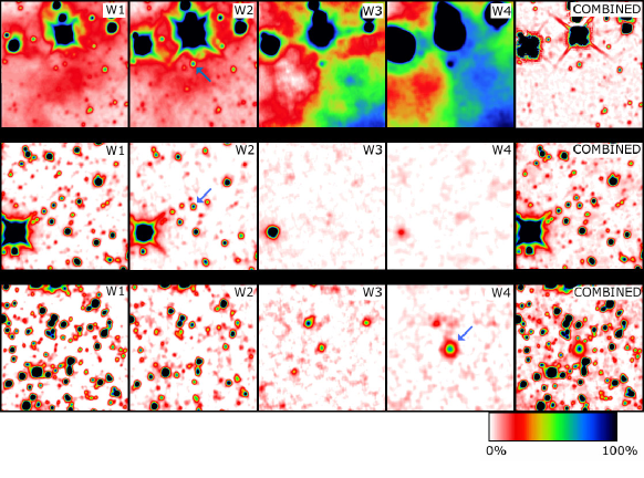
Figure 2: Examples of the use of MDET for combining images at multiple wavelengths to increase detection sensitivity. Top row: Young stellar object (YSO); Middle row: Ultra-cool brown dwarf (BD); Bottom row: Hyper-Luminous InfraRed Galaxy (HyLIRG). Coadded images, each with $5^{\prime}\times 5^{\prime}$ field of view, are shown for the four WISE wavebands, W1 (3.4 $\mu$m), W2 (4.6 $\mu$m), W3 (12 $\mu$m), and W4 (22 $\mu$m); these were combined to produce the optimal detection image (labeled “COMBINED”) shown at the right of each row. For each of the three objects, all five images are presented on the same (linear) intensity scale in units of $S/N$, whose peak values are 102, 68, and 33 for the YSO, BD, and LyLIRG, respectively. In each case, the object of interest is indicated by the blue arrow for the waveband with highest $S/N$ (W2 for the YSO and brown dwarf; W4 for the HyLIRG).

in one band only. The example does, however, demonstrate that non-detection in the three “dropout” bands did not contaminate the detection. The third example (HyLIRG) represents a combination of both circumstances, since the source is detected in only two of the four bands. Nevertheless, the two bands in which the source is detected have served to increase the source $S/N$ in the combined image, while the two dropout bands have not appreciably contaminated the result.

Overall, the use of MDET as the initial detection step has benefited WISE photometry in the following ways:

• The detection sensitivity has been increased for the reasons discussed above. This increase does not come at the expense of reliability, since the image combination process tends to average out the noise bumps. The inferred reliability meets the WISE Functional Requirement value of 99.9% for SNR $>$ 20 (Cutri et al. 2011).

• The fact that a single position is supplied for each source, even though the source is detected in multiple bands, facilitates simultaneous multiband parameter estimation. The advantages of the latter are that no bandmerging is required (thus avoiding band-to-band matching ambiguities crowded fields), and that dropout bands automatically receive a flux upper limit.

4 Application to ASKAP

MDET can facilitate the optimal detection of faint sources by combining images along the frequency axis of an ASKAP data cube without introducing biases which favor one spectral shape over another. However, because of the limited frequency range of ASKAP (700-1800 MHz receiver range; 300 MHz correlator bandwidth), the benefits of the algorithm would be realized to a much larger extent for sources whose spectra contain narrow-band features than for sources with broadband spectra. As an example of the latter, consider a typical AGN whose flux density spectrum in the ASKAP frequency range is of the approximate form $S_{\nu}\propto\nu^{-1}$. Although the combining of images over all ASKAP channels will increase the $S/N$ by approximately the square root of the number of channels involved, the same will also be true for a uniformly-weighted linear combination of images of such a source. In fact, for a source with a similar spectral index, the improvement in $S/N$ afforded by MDET over that obtained with the linear combination would be less than 4%. The situation is radically different for spectroscopy, however, and we now discuss an important potential application.

A major scientific goal for ASKAP and SKA is the detection of neutral hydrogen in distant galaxies, an important aspect of the study of galaxy formation and evolution (Johnston et al. 2008; Rawlings et al. 2004). The MDET procedure could be used to advantage in such searches by providing a spectrally neutral way to combine the images for all narrow-band channels within the frequency range corresponding to a given range of redshifts. As an example, we consider the combination of signals from a WALLABY data cube whose spectral sampling interval corresponds to 4 km s^-1. We suppose that somewhere in the redshift range $z<0.1$ is the signal from a velocity-broadened HI line, a typical width for which might be $\sim 400$ km s^-1 (Koribalski 1996). Since the achievable gain in detectability increases monotonically with the per-channel $S/N$ of the spectral peaks of the source, it is desirable to carry out the detection step at a spectral resolution commensurate with the spectral structure of interest, so that some boxcar averaging of the spectral channels may be warranted. In the present example, combining the raw channels in groups of 25 would result in an effective channel width of 100 km s^-1, so that our source signal would be spread over 4 such channels. For a peak $S/N$ per channel $\sim 10$, an unweighted linear combination of these channels would then produce a signal with $S/N\sim 2$, i.e., barely detectable, whereas the MDET procedure would result in $S/N\sim 12$. Of course, the peak signal from a properly-tuned spectral matched filter would be even greater, but we would then be optimizing for a particular line width and shape, and be less sensitive to other potentially interesting structure. For example, if optimized for 100 km s^-1 structure, the spectral matched filter could do no better than $S/N\sim 10$. While this numerical example was illustrative only, we can make the general statement that by combining images from WALLABY data cubes using the MDET procedure, we obtain an optimal answer to the question: In which portions of the field of view are the observations inconsistent with random noise?

With an appropriate sign change in Equation (14), the procedure could be applied to the detection of HI absorption, and therefore be of potential benefit to the processing of data from the FLASH project in the redshift range $0.5<z<1.0$. Ultimately, it is expected that the full SKA will enable detection out to $z\sim 2.5$ (Zwaan 2006). At such high redshifts, the emission is too weak to detect the HI clouds of individual galaxies. The problem can be mitigated, however, by combining the HI images of overlapping clouds of galaxies with known redshifts (Khandai et al. 2011). This approach enabled Chang et al. (2010) to detect neutral hydrogen out to $z=0.8$. MDET has the potential for further improving this technique, since it provides a way of combining the images without prior knowledge of the redshifts of individual clouds.

5 Conclusions

MDET provides a procedure for combining the narrow-band images within a data cube in such a way as to increase optimally the detection signal to noise ratio without introducing a color bias. We have used it successfully in the WISE mission, and believe it will be of substantial benefit to ASKAP, particularly for sources with narrow-band spectral features. In particular, we suggest that it could aid in the detection of neutral hydrogen in distant galaxies.

References

- Chang et al. (2010) Chang, T.-C., Pen, U.-L., Bandura, K., & Peterson, J. B. 2010, Nature, 466, 463
- Cutri et al. (2011) Cutri, R. M. et al. 2011, “Explanatory Supplement to the WISE Preliminary Release,” http://wise2.ipac.caltech.edu/docs/release/prelim/expsup
- Jarrett et al. (2011) Jarrett, T. H. et al., 2011, ApJ, 735, 112
- Johnston et al. (2008) Johnston, S. et al. 2008, “Science With ASKAP,” arXiv:0810.5187
- Johnston et al. (2009) Johnston, S., Feain, I. J., & Gupta, N. 2009, in “The Low-Frequency Radio Universe,” ASP Conf. Series, Vol. LFRU, 2009; Eds: D.J. Siakia, Dave Green, Y Gupta and Tiziana Venturi
- Khandai et al. (2011) Khandai, N., Sethi, S. K., DiMatteo, T. & 4 coauthors, 2011, MNRAS, in press
- Koribalski (1996) Koribalski, B. 1996, ASPC, 106, 238
- Mainzer et al. (2011) Mainzer, A., Cushing, M. C., Skrutskie, M. & 16 co-authors, 2011, ApJ, 726, 30
- Rawlings et al. (2004) Rawlings, S., Abdalin, F. B., Bridle, S. L. & 4 coauthors, 2004, in “Science with the Square Kilometre Array”
- Szalay et al. (1999) Szalay, A. S., Connolly, A. J., & Szololy, G. P. 1999, AJ, 117, 68
- Wright et al. (2010) Wright, E. L. et al. 2010, AJ, 140,1868
- Zwaan (2006) Zwaan, M. 2006, in “Cosmology, Galaxy Formation and Astroparticle Physics on the Pathway to the SKA,” Klöckner, H.-R., Jarvis, M. & Rawlings, S. (eds), Oxford, U.K.