Transport anisotropy of the pnictides studied via
Monte Carlo simulations of a Spin-Fermion model

Abstract

An undoped three-orbital Spin-Fermion model for the Fe-based superconductors is studied via Monte Carlo techniques in two-dimensional clusters. At low temperatures, the magnetic and one-particle spectral properties are in agreement with neutron and photoemission experiments. Our main results are the resistance vs. temperature curves that display the same features observed in BaFe₂As₂ detwinned single crystals (under uniaxial stress), including a low-temperature anisotropy between the two directions followed by a peak at the magnetic ordering temperature, that qualitatively appears related to short-range spin order and concomitant Fermi Surface orbital order.

Introduction. In early studies of Fe-based superconductors review , it was widely assumed that Fermi Surface (FS) nesting was sufficient to understand the undoped-compounds magnetic order with wavevector ${\bf Q}$ = ($\pi$,0) cruz and the pairing tendencies upon doping. Neutron scattering reports of spin-incommensurate order spinIC are in fact compatible with the nesting scenario. However, several recent experimental results cannot be explained by FS nesting, including (i) electronic “nematic” tendencies in Ca(Fe_1-xCo_x)₂As₂ davis ; (ii) orbital-independent superconducting gaps shimojima found using laser angle-resolved photoemission (ARPES) spectroscopy on BaFe₂(As_0.65P_0.35)₂ and Ba_0.6K_0.4Fe₂As₂; and, more importantly for the investigations reported here, (iii) the report of local moments at room temperature ($T$) via Fe X-ray emission spectroscopy local ; mannella . Considering these experiments and others, a better characterization of the pnictides is that they are in the “middle” between the weak and strong Coulomb correlation limits basov ; rong ; kotliar . Because this intermediate Hubbard $U$ range is difficult for analytical approaches, there is interest in the development of simpler models that can be studied via computational techniques to provide insight into such a difficult coupling regime. The Hartree-Fock (HF) approximation to the Hubbard model luo cannot be applied at room $T$ since HF approximations only lead to non-interacting fermions above the ordering temperature $T_{\rm N}$, and thus the local moment physics local cannot be reproduced qmc .

Recently, a Spin-Fermion (SF) model for the pnictides has been independently proposed by Lv et al. Kruger and Yin et al. SF . The model, very similar to those widely discussed for manganites, originally involved itinerant electrons in the $xz$ and $yz$ $d$-orbitals coupled, via an on-site Hund interaction, to local spins (assumed classical) that represent the magnetic moment of the rest of the Fe orbitals (considered localized). The Hund interaction is supplemented by a nearest-neighbor (NN) and next-NN (NNN) classical Heisenberg spin-spin interaction. This SF model has interesting features that makes it qualitatively suitable for the pnictides, particularly since by construction the model has itinerant electrons in interaction with local moments local ; mannella at all temperatures.

Phenomenological SF models have been proposed before for underdoped cuprates, with itinerant fermions representing carriers locally coupled to classical spins representing the antiferromagnetic order parameter. These investigations unveiled stripe tendencies SF-cuprates1 , ARPES and optical conductivity results SF-cuprates2 similar to experiments, and even the dominance of the $d$-wave channel in pairing SF-cuprates3 . Thus, it is natural to apply now these ideas to the Fe superconductors.

As remarked already, SF models are also mathematically similar to models used for the manganites Dagotto . Then, all the experience accumulated in the study of Mn-oxides can be transferred to the analysis of SF models for Fe-superconductors. In particular, one of our main objectives is to study for the first time a SF model for pnictides employing Monte Carlo (MC) techniques, allowing for an unbiased analysis of its properties. Moreover, to test the model, challenging experimental results will be addressed. It is known that for detwinned Ba(Fe_1-xCo_x)₂As₂ single crystals, a puzzling transport anisotropy has been discovered between the ferromagnetic (FM) and antiferromagnetic (AFM) directions Chu . In addition, the resistivity vs. $T$ curves display an unexpected peak at $T_{\rm N}$$\sim$130 K, and the presumably weak effect of an applied uniaxial stress Chu still causes the anisotropy to persist well beyond $T_{\rm N}$. However, recent neutron results suggest that the transport anisotropy may be actually caused by strain effects that induce a shift upwards of the tetragonal-orthorhombic and $T_{\rm N}$ transitions wilson ; blomberg , as opposed to a spontaneous rotational symmetry-breaking state not induced by magnetism or lattice effects. Then, theoretical guidance is needed. While the low-$T$ anisotropy was already explained as caused by the coupling between the spins and orbitals in the ${\bf Q}$=$(\pi,0)$ state zhang , the full transport curves at finite $T$ define a challenge that will be here addressed for the nontrivial undoped case.

Model and Method. The SF model Kruger ; SF is given by

$$H_{\rm SF}=H_{\rm Hopp}+H_{\rm Hund}+H_{\rm Heis}.$$ (1)

The first term $H_{\rm Hopp}$ describes the Fe-Fe hopping of itinerant electrons. To better reproduce the band structure of pnictides review , three $d$-orbitals ($xz$, $yz$, $xy$) will be used instead of two. The full expression for $H_{\rm Hopp}$ is cumbersome to reproduce here, but it is sufficient for the readers to consult Eqs.(1-3) and Table I of Ref. three, for the mathematical form and the actual values of the hoppings in eV’s. The density of relevance used here is $n$=4/3 three . The Hund interaction is simply $H_{\rm Hund}$=$-J_{\rm H}\sum_{{\bf i}\alpha}{{{\bf S}_{\bf i}}\cdot{{{\bf s}^{\alpha}}_{\bf i}}}$, with ${\bf S}_{\bf i}$ the classical spin at site ${\bf i}$ ($|{\bf S}_{\bf i}|$=1), and ${{\bf s}^{\alpha}}_{\bf i}$ the itinerant-fermion spin of orbital $\alpha$ comment-hund . The last term $H_{\rm Heis}$ contains the spin-spin interaction among the localized spins $H_{\rm Heis}$=$J_{\rm NN}\sum_{\langle{\bf ij}\rangle}{{{\bf S}_{\bf i}}\cdot{{\bf S}_{\bf j}}}$ + $J_{\rm NNN}\sum_{\langle\langle{\bf im}\rangle\rangle}{{{\bf S}_{\bf i}}\cdot{{\bf S}_{\bf m}}}$, where $\langle\rangle$ ($\langle\langle\rangle\rangle$) denotes NN (NNN) couplings. The particular ratio $J_{\rm NNN}$/$J_{\rm NN}$=2/3 was used in all the results below, leading to $(\pi,0)$/$(0,\pi)$ magnetism comment . Any other ratio $J_{\rm NNN}$/$J_{\rm NN}$ larger than 1/2 would have been equally suitable for our purposes.

The well-known Monte Carlo (MC) technique for SF models Dagotto will be here used to study $H_{\rm SF}$ at any $T$. In this technique, the acceptance-rejection MC steps are carried out in the classical spins, while at each step a full diagonalization of the fermionic sector (hopping plus on-site Hund terms) for fixed classical spins is performed via library subroutines in order to calculate the energy of that spin configuration. These frequent diagonalizations render the technique CPU-time demanding. The simulation is run on a finite 8$\times$8 cluster with periodic boundary conditions (PBC) and uses the full $H_{\rm SF}$ model for the MC time evolution and generation of equilibrated configurations for the classical spins at a fixed $T$ MCsteps . However, for the MC measurements those equilibrated configurations are assumed replicated in space but differing by a phase factor such that a better resolution is reached with regards to the momentum ${\bf k}$. Since a larger lattice with more eigenstates gives a more continuous distribution of eigenenergies, the procedure then reduces finite-size effects in the measurements. This well-known method is often referred to as “Twisted” Boundary Conditions (TBC) salafranca . In practice, phases $\Phi$ are added to the hopping amplitudes, schematically denoted as “$t$”, at the boundary via $t_{TBC}$=$e^{i\Phi}t$, with $\Phi$=$2\pi m/M$ ($m$=0,1,…,$M-1$) such that the number of possible momenta in the $x$ or $y$ directions becomes $L$=8$\times$$M$.

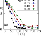
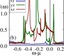
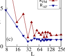
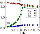
Figure 1: (color online) (a) Classical spins structure factor S($\pi$,0) (normalized to 1) vs. $T$, for the $J_{\rm H}$’s indicated, using the PBC 8$\times$8 cluster and $J_{\rm NN}$=0.015. The oscillations in the data are indicative of the error bars. (b) Density of states $N(\omega)$ of each orbital ($\mu$= chemical potential), using TBC with $L$=512, at $T$=0 K and $J_{\rm H}$=0.1 eV, for the perfect $(\pi,0)$ magnetic state. (c) Resistance $R$ vs. $L$ (TBC 8$\times$8) for the FM and AFM directions of the perfect $(\pi,0)$ magnetic state ($J_{\rm H}$=0.1 eV). (d) The occupation at the FS $n(\mu)$ (see text) of the three orbitals vs. $T$, using $L$=256. A coupling $J_{\rm NN}$=0.016 (0.014) along the $x$ ($y$) axis was used (see text).

Results. Figure 1(a) contains MC results for the structure factor of the classical spins, defined as $S({\bf q})$=${1}\over{N^{2}}$$\sum_{{\bf i},{\bf j}}\langle{{\bf S}_{\bf i}}\cdot{{\bf S}_{\bf j}}\rangle e^{i{\bf q}\cdot{({\bf i-j}})}$ ($N$ = number of sites), illustrating the development of ${\bf Q}$=$(\pi,0)$ magnetic order as $T$ is reduced. Since a ratio $J_{\rm NNN}$/$J_{\rm NN}$$>$1/2 is “frustrating”, finding ${\bf Q}$-order at $J_{\rm H}$=0 is not surprising, but Fig. 1 shows that this order remains stable turning on $J_{\rm H}$ in the range investigated, as opposed to inducing transitions to other states. The chosen value of $J_{\rm NN}$ in Fig. 1(a) leads to a $T_{\rm N}$ similar to that in BaFe₂As₂. The low-$T$ orbitally-resolved electronic density-of-states (DOS) is in Fig. 1(b). The ${\bf Q}$ magnetic order opens a pseudogap (PG) in the $yz$ orbital, while the others are not much affected. This PG generation was previously discussed when contrasting theory and ARPES experiments weight and it should not be confused with long-range orbital-order, that in this SF model occurs at $J_{\rm H}$$\sim$0.4 or larger.

Figure 1(c) contains the evolution of the 8$\times$8-cluster resistance $R$ increasing the number of momenta via the TBC, calculated via standard procedures Dagotto ; Verges . While the ratio of $R$’s along the FM and AFM directions is always $>1$, i.e. qualitatively correct, TBC with $L$=256 is needed to reach stable values. In addition, the occupation of the three orbitals at the FS (Fig. 1(d)) was defined as $n(\mu)$=$\int d\epsilon n(\epsilon)\beta e^{\beta(\epsilon-\mu)}/(1+e^{\beta(\epsilon-\mu)})^{2}$, involving the $\mu$-derivative of the fermionic population. As $T$ increases and the ${\bf Q}$ order weakens, the $xz$-$yz$ orbitals populations converge to the same values.

The results of Fig. 1, and others below, were obtained introducing a “small” explicit asymmetry along the $x$ and $y$ axes for $J_{\rm NN}$, namely a generalized $J^{\alpha}_{\rm NN}$ ($\alpha$=$x,y$) was used. Its purpose is to mimic the orthorhombic distortion and strain effects cruz ; wilson ; blomberg and judge if the present calculations reproduce transport experiments Chu ; wilson ; blomberg . Consider the ratio $r_{\rm NN}$=$J^{x}_{\rm NN}$/$J^{y}_{\rm NN}$. Using the dependence of the hopping amplitudes with the distance $u$ between $d$- and $p$-orbitals i.e. $t_{pd}$$\sim$$1/u^{7/2}$ harrison , the angles involved in the Fe-As-Fe bonds, the low-$T$ lattice parameters cruz , fourth-order perturbation in the hoppings for the Fe-Fe superexchange, and, more importantly, neglecting contributions of the $yz$ orbital that is suppressed at the Fermi level weight as long as $(\pi,0)$ spin fluctuations dominate leads to a crude estimation $r_{\rm NN}$$\sim$1.4. Since this is likely an upper bound, the ratio used in our MC simulation $r_{\rm NN}$$\sim$1.14, assumed to be temperature independent, is reasonable. Other crude estimations including the direct Fe-Fe hoppings harrison or employing the lattice parameters under pressure wilson lead to similar ratios. Then, our asymmetry value is qualitatively realistic.

Figure 2: (color online) $A({\bf k},\omega)$ at $\omega$=$\mu$ (TBC 8$\times$8 $L$=512). The model used (see Ref. three, ) includes the staggered As modulation out of the FeAs layer. Thus, our results are in the folded Brillouin zone convention, and for this reason two electron pockets (as opposed to just one) are centered at X in the panels above. The pocket elongated vertically at X would corresponds to a pocket at Y in the unfolded convention if the As modulation is considered via a quasicrystal momentum three . (a-c) are for $J_{\rm H}$=0.1 eV. Red, green, and blue are for the $xz$, $yz$, and $xy$ orbitals, respectively. (a) $T$=$40K$, below $T_{\rm N}$. The $(\pi,0)$ magnetic order induces $yz$-orbital electron satellite pockets. (b) $T$=$110K$$\sim$$T_{\rm N}$. In this regime, the MC configurations display small coexisting patches of $(\pi,0)$ and $(0,\pi)$ order (see text), creating almost symmetric $xz$ and $yz$ features around $\Gamma$. (c) Large $T$=$360$ K, with no remnants of the $(\pi,0)$ order. The FS becomes a broaden version of the non-interacting FS at $J_{\rm H}$=$0$, shown in (d) at $T$=100 K.

Previous investigations luo showed that the $T$=0 HF approximation to the undoped multiorbital Hubbard model can reproduce neutron diffraction results and ARPES data. A similar degree of accuracy should be expected from any reasonable model for the pnictides, including $H_{\rm SF}$. To test this assumption, the one-particle spectral function $A({\bf k},\omega)$ was calculated, and the FS at different $T$’s is shown in Fig. 2, contrasted against the low-$T$ fermionic non-interacting limit $J_{\rm H}$=$0$. At low-$T$ in the ordered state the expected asymmetry between the $(\pi,0)$ and $(0,\pi)$ electron pockets is observed (not shown), and more importantly satellite pockets (with electron character) develop close to the $\Gamma$ hole pockets (Fig. 2(a)), as in ARPES experiments luo ; arpes . Thus, the SF model studied here passes the low-$T$ ARPES test. As $T$ increases, at or well above $T_{\rm N}$ (Figs. 2(b) and (c)) the $xz$ and $yz$ differences are reduced and rotational invariance is recovered, albeit with a FS broader than in the non-interacting low-$T$ limit (Fig. 2(d)).

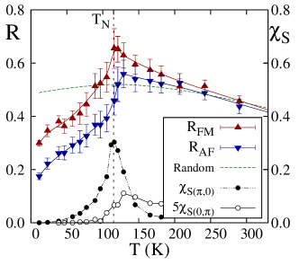
Figure 3: (color online) Resistance $R$ of the SF model calculated via MC simulations, at $J_{\rm H}$=0.1 eV and using the $L$=256 TBC 8$\times$8 cluster. $T_{\rm N}$ is indicated, and the magnetic susceptibilities $\chi_{S}$ are also shown. The FM-AFM directions asymmetry is evident at low $T$ (note that the FM and AFM labels simply refer to the $y$ and $x$ directions, respectively, and not to fully FM or AFM spin configurations). As $T$ increases the symmetry is restored, and the curves display a peak at $T_{\rm N}$. A small symmetry-breaking difference $r_{\rm NN}$=1.14 is used (see text). In green (dashed line) are the results for random spin configurations, showing that their $R$ is smaller than in the MC results near $T_{\rm N}$. The width of the $\chi$ peaks extend to $\sim$1.5$T_{\rm N}$, in agreement with neutron scattering for CaFe₂As₂ diallo .

$R$ vs. $T$ curves. Our most important result is the $T$ dependence of $R$ along the two axes, shown in Fig. 3. It is visually clear that these results are similar to the transport data of Ref. Chu, , particularly after realizing that lattice effects, that cause the continuous raise of $R$ with $T$ in the experiments, are not incorporated in the SF model. A clear difference exists between the FM and AFM directions at low $T$, induced by the $(\pi,0)$ magnetic order that breaks spontaneously rotational invariance. At low $T$, this difference was understood in the Hubbard-model HF approximation zhang based on the reduction of the $yz$ orbital population (Fig. 1(d)). This explanation is equally valid in the SF model, and at low $T$ the SF model and the Hubbard model, when treated via the HF approximation, lead to similar physics.

The most interesting result in Fig. 3 is the development of a peak at $T_{\rm N}$, and the subsequent slow convergence of $R$ toward similar values along both directions with further increasing $T$ (as already discussed, to model better the effect of uniaxial stress Chu , a weak symmetry-breaking difference between the NN Heisenberg couplings along $x$ and $y$ was included). To our knowledge, this is the first time that the full $R$ vs. $T$ curve is successfully reproduced via computational studies.

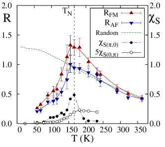
Figure 4: (color online) Resistance $R$ calculated using a $L$=64 TBC 16$\times$16 cluster, with $J_{\rm NN}$=0.032 (0.028) along the $x$ ($y$) axis. The spin configurations are generated via $H_{\rm Heis}$, while the $R$ measurements use the full $H_{\rm SF}$, at $J_{\rm H}$=0.1 eV. The rest of the notation is as in Fig. 3.

A study as in Fig. 3 using a larger cluster, e.g. 16$\times$16, is not practical since the computer time grows like $N^{4}$ ($N$=number of sites), leading to an effort 256 times larger. However, results as in Fig. 1(a) indicate that the classical spins configurations generated merely by the spin-spin interaction could be qualitatively similar to those generated by the full SF model, as long as $J_{\rm H}$ does not push the system into a new phase. Thus, the MC evolution could be carried out with $H_{\rm Heis}$ only, while measurements can still be performed using the full diagonalization of $H_{\rm SF}$. Such measurements (very CPU-time consuming) must be sufficiently sparsed in the MC evolution to render the process practical. This procedure was implemented on a TBC 16$\times$16 cluster, with $L$=64 comment2 . The results for $R$ are in Fig. 4, and they show a remarkable similarity with Fig. 3, and with experiments. Thus, the essence of the $R$ vs. $T$ curves is captured by electrons moving in the spin configurations generated by $H_{\rm Heis}$. Size effects are small in the range analyzed here.

What causes the increase of $R$ upon cooling before $T_{\rm N}$ is reached, displaying insulating characteristics? Since our results are similar to experiments, an analysis of the MC-equilibrated configurations may provide qualitative insight into their origin. In Fig. 5(a), a typical MC configuration of classical spins is shown. The colors at the links illustrate the relative orientation of the two spins at the ends. The $(\pi,0)$ long-range order is lost, but individual spins are not randomly oriented. In fact, the state contains small regions resembling locally either a $(\pi,0)$ or $(0,\pi)$ order (short-range spin order), and $S({\bf q})$ still displays broad peaks at those two wavevectors. In standard mean-field approximations there are no precursors of the magnetic order above $T_{\rm N}$, but in the SF model there are short-range fluctuations in the same regime.

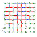
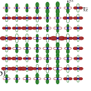
Figure 5: (color online) (a) Typical MC-generated classical spin configuration on an 8$\times$8 cluster at $T_{\rm N}$$\sim$110 K, $J_{\rm H}$=0.1 eV, and $J_{\rm NN}$=0.016 (0.014) along the $x$ ($y$) axis. The red (blue) lines denote AFM (FM) NN correlations, of intensity proportional to the width. (b) The dominant orbital at the FS at each site for the configuration used in (a), calculated using $n(\mu)$ as in Fig. 1(d). Red (green) denote the $xz$ ($yz$) orbital, with a size proportional to the density.

States with “spin patches” as in Fig. 5(a) lead to a concomitant patchy orbital order at the FS shown in Fig. 5(b), where the most populated orbital at $\mu$ at every site, either $xz$ or $yz$, are indicated. The orbital orientation suggests that the $xz$ ($yz$) FS population favors transport along the $x$ ($y$) axis. The patchy order should have a resistance larger than that of a randomly-oriented spin background. This is confirmed by calculating $R$ vs. $T$ in the absence of a guiding Hamiltonian, i.e. by generating random spin configurations. The results are in Figs. 3 and 4 (green dashes) and their values are indeed below those of the peak resistance at $T_{\rm N}$ of the full SF model, i.e. with configurations as in Fig. 5. Then, the effect of strain coupled to short-range spin and FS orbital order appears to be the cause of the peak in the $R$ vs. $T$ curves fernandez ; comment-asym . Using a smaller (but nonzero) anisotropy, the $R$-$T$ curves display a concomitantly smaller anisotropy, but still they have a small peak at $T_{\rm N}$ (not shown). Thus, the patchy states may also explain the insulating properties of Fe_1.05Te FT and (Tl,K)Fe_2-xSe₂ KFS above $T_{\rm N}$.

Conclusions. The Spin-Fermion model for pnictides was here studied with MC techniques. The magnetic and ARPES properties of the undoped compounds are well reproduced. Including a small explicit symmetry breaking to account for strain effects, the resistance $R$ vs. $T$ curves are qualitatively similar to those observed for BaFe₂As₂ Chu , including a peak at $T_{\rm N}$ that appears caused by short-range spin and FS orbital order. In our calculations, the anisotropy above $T_{\rm N}$ exists only as long as a strain distortion exists, compatible with results for annealed BaFe₂As₂ samples pnas . This successful application of a SF model paves the way to more demanding efforts involving doped systems where anisotropy effects are stronger than in the undoped limit Chu .

Acknowledgment. The authors thank I.R. Fisher, M. Daghofer, S. Dong, W. Lv, S. Wilson, X. Zhang, Q. Luo, and A. Nicholson for useful discussions. This work was supported by the US Department of Energy, Office of Basic Energy Sciences, Materials Sciences and Engineering Division, and also by the National Science Foundation under Grant No. DMR-11-04386 (S.L., C.S., A.M., E.D.). G.A. was supported by the Center for Nanophase Materials Sciences, sponsored by the Scientific User Facilities Division, BES, U.S. DOE. This research used resources of the National Center for Computational Sciences, as well as the OIC at ORNL.

References

- (1) D. C. Johnston, Adv. Phys. 59, 803 (2010).
- (2) C. de la Cruz, Q. Huang, J. Lynn, I. Ratcliff, J. Zaretsky, H. Mook, G. Chen, J. Luo, N. Wang, and P. Dai, Nature (London) 453, 899 (2008).
- (3) D. K. Pratt, M. G. Kim, A. Kreyssig, Y. B. Lee, G. S. Tucker, A. Thaler, W. Tian, J. L. Zarestky, S. L. Bud’ko, P. C. Canfield, B. N. Harmon, A. I. Goldman, and R. J. McQueeney, Phys. Rev. Lett. 106, 257001 (2011).
- (4) T.-M. Chuang, M. P. Allan, J. Lee, Y. Xie, N. Ni, S. L. Bud’ko, G. S. Boebinger, P. C. Canfield, and J. C. Davis, Science 327, 181 (2010).
- (5) T. Shimojima, F. Sakaguchi, K. Ishizaka, Y. Ishida, T. Kiss, M. Okawa, T. Togashi, C.-T. Chen, S. Watanabe, M. Arita, K. Shimada, H. Namatame, M. Taniguchi, K. Ohgushi, S. Kasahara, T. Terashima, T. Shibauchi, Y. Matsuda, A. Chainani, and S. Shin, Science 332, 564 (2011).
- (6) H. Gretarsson, A. Lupascu, J. Kim, D. Casa, T. Gog, W. Wu, S. R. Julian, Z. J. Xu, J. S. Wen, G. D. Gu, R. H. Yuan, Z. G. Chen, N.-L. Wang, S. Khim, K. H. Kim, M. Ishikado, I. Jarrige, S. Shamoto, J.-H. Chu, I. R. Fisher, and Y-J. Kim, Phys. Rev. B 84, 100509(R) (2011).
- (7) F. Bondino, E. Magnano, M. Malvestuto, F. Parmigiani, M. A. McGuire, A. S. Sefat, B. C. Sales, R. Jin, D. Mandrus, E. W. Plummer, D. J. Singh, and N. Mannella, Phys. Rev. Lett. 101, 267001 (2008).
- (8) M. M. Qazilbash, J. J. Hamlin, R. E. Baumbach, Lijun Zhang, D. J. Singh, M. B. Maple, and D. N. Basov, Nat. Phys. 5, 647 (2009).
- (9) R. Yu, K.T. Trinh, A. Moreo, M. Daghofer, J. Riera, S. Haas, and E. Dagotto, Phys. Rev. B 79, 104510 (2009).
- (10) Z.P. Yin, K. Haule, and G. Kotliar, Nat. Mat. 10, 932 (2011).
- (11) Q. Luo, G. Martins, D.-X. Yao, M. Daghofer, R. Yu, A. Moreo, and E. Dagotto, Phys. Rev. B 82, 104508 (2010).
- (12) Determinantal MC cannot be applied to the multiorbital case due to the “sign problem” even in the undoped limit.
- (13) W. Lv, F. Krüger, and P. Phillips, Phys. Rev. B 82, 045125 (2010).
- (14) W.-G. Yin, C.-C. Lee, and W. Ku, Phys. Rev. Lett. 105, 107004 (2010).
- (15) C. Buhler, S. Yunoki, and A. Moreo, Phys. Rev. Lett. 84, 2690, (2000).
- (16) M. Moraghebi, C. Buhler, S. Yunoki and A. Moreo, Phys. Rev. B 63, 214513 (2001); M. Moraghebi, S. Yunoki and A. Moreo, Phys. Rev. B 66, 214522 (2002).
- (17) M. Moraghebi, S. Yunoki, and A. Moreo, Phys. Rev. Lett. 88, 187001 (2002).
- (18) E. Dagotto, T. Hotta, and A. Moreo, Phys. Rep. 344, 1 (2001).
- (19) J-H. Chu, J. G. Analytis, K. De Greve, P.L. McMahon, Z. Islam, Y. Yamamoto, and I.R. Fisher Science 13, 824 (2010). See also I.R. Fisher, L. Degiorgi, and Z.X. Shen, Rep. Prog. Phys. 74, 124506 (2011).
- (20) C. Dhital, Z. Yamani, Wei Tian, J. Zeretsky, A. S. Sefat, Ziqiang Wang, R. J. Birgeneau, and S. D. Wilson, Phys. Rev. Lett. 108, 087001 (2012).
- (21) E. C. Blomberg, A. Kreyssig, M. A. Tanatar, R. Fernandes, M. G. Kim, A. Thaler, J. Schmalian, S. L. Bud’ko, P. C. Canfield, A. I. Goldman, and R. Prozorov, Phys. Rev. B 85, 144509 (2012).
- (22) X. Zhang and E. Dagotto, Phys. Rev. B 84, 132505 (2011).
- (23) M. Daghofer, A. Nicholson, A. Moreo, and E. Dagotto, Phys. Rev. B 81, 014511 (2010).
- (24) Although the fermions do not have a direct Hund interaction among themselves, an effective one is generated via the interaction with the classical variables (more formally, “integrating out” the classical spins should induce a Hund coupling among the fermions).
- (25) The transition from order to / order occurs at /=1/2, within .
- (26) Typically 20,000 MC sweeps through the lattice are used for thermalization followed by 10,000 for the measurements that occur every 20 configurations.
- (27) J. Salafranca, G. Alvarez, and E. Dagotto, Phys. Rev. B 80, 155133 (2009).
- (28) M. Daghofer, Q.-L. Luo, R. Yu, D. X. Yao, A. Moreo and E. Dagotto, Phys. Rev. B 81, 180514(R) (2010).
- (29) J. A. Vergés, Comput. Phys. Commun. 118, 71 (1999).
- (30) W.A. Harrison, Electronic Structure and the Properties of Solids, (Dover, 1989).
- (31) M. Yi, D.H. Lu, J.G. Analytis, J.-H. Chu, S.-K. Mo, R.-H. He, M. Hashimoto, R. G. Moore, I.I. Mazin, D.J. Singh, Z. Hussain, I.R. Fisher, and Z.-X. Shen, Phys. Rev. B 80, 174510 (2009).
- (32) S.O. Diallo, D.K. Pratt, R.M. Fernandes, W. Tian, J.L. Zarestky, M. Lumsden, T.G. Perring, C.L. Broholm, N. Ni, S.L. Bud’ko, P.C. Canfield, H.-F. Li, D. Vaknin, A. Kreyssig, A.I. Goldman, and R.J. McQueeney, Phys. Rev. B 81, 214407 (2010).
- (33) 200,000 (100,000) MC steps for thermalization (measurements) were employed. The calculations are very CPU time consuming, thus only 20 were performed, but self-averaging effects render the error bars small.
- (34) The resistivity anisotropy has also been recently explained in similar terms via a nematic phase above (R.M. Fernandes, E. Abrahams, and J. Schmalian, Phys. Rev. Lett. 107, 217002 (2011)). The existence of a nematic phase in the SF model will be studied in the future.
- (35) This qualitative argumentation should be substantiated by transport calculations involving, e.g., scattering rates.
- (36) G. F. Chen, Z. G. Chen, J. Dong, W. Z. Hu, G. Li, X. D. Zhang, P. Zheng, J. L. Luo, and N. L. Wang, Phys. Rev. B 79, 140509(R) (2009).
- (37) M. H. Fang, H. D.Wang, C. H. Dong, Z. J. Li, C. M. Feng, J. Chen, and H. Q. Yuan, EPL 94, 27009 (2011).
- (38) M. Nakajima, T. Liang, S. Ishida, Y. Tomioka, K. Kihou, C. H. Lee, A. Iyo, H. Eisaki, T. Kakeshita, T. Ito, and S. Uchida, PNAS 108, 12238 (2011).