Formation times, mass growth histories and concentrations of dark matter haloes

Abstract

We develop a simple model for estimating the mass growth histories of dark matter halos. The model is based on a fit to the formation time distribution, where formation is defined as the earliest time that the main branch of the merger tree contains a fraction $f$ of the final mass $M$. Our analysis exploits the fact that the median formation time as a function of $f$ is the same as the median of the main progenitor mass distribution as a function of time. When coupled with previous work showing that the concentration $c$ of the final halo is related to the formation time $t_{f}$ associated with $f\sim 0.04$, our approach provides a simple algorithm for estimating how the distribution of halo concentrations may be expected to depend on mass, redshift and the expansion history of the background cosmology. We also show that one can predict $\log_{10}c$ with a precision of about 0.13 and 0.09 dex if only its mass, or both mass and $t_{f}$ are known. And, conversely, one can predict $\log_{10}t_{f}$ from mass or $c$ with a precision of 0.12 and 0.09 dex, approximately independent of $f$. Adding the mass to the $c$-based estimate does not result in further improvement. These latter results may be useful for studies which seek to compare the age of the stars in the central galaxy in a halo with the time the core was first assembled.

1 Introduction

One main focus of modern observational cosmology is the study of the uabundance and structural properties of galaxy clusters: typically, the abundance is expressed as a function of mass $M$, and the structural property of most interest is the central concentration $c$ of the mass density profile. There are various ongoing and planned surveys which are capable of finding thousands of clusters using well-controlled/calibrated selection criteria, so a number of large homogeneous samples of galaxy clusters will be available in the near future (Laureijs et al., 2011). Such samples have the potential to strongly constrain the fundamental parameters of a given cosmological model (e.g. $\Lambda$CDM). This is in large part because of numerical simulations (Navarro et al., 1997, e.g.) which have shown that, at fixed mass, halos are less concentrated if the matter density, $\Omega_{m}$, is lower. In addition, for a given cosmology, there is a reasonably tight monotonic correlation between $M$ and $c$, although this $M-c$ relation depends on how $c$ is estimated. Recently Prada et al. (2011) report that, if $c$ is determined by fitting to the circular velocity rather than the density profile, then the $c-M$ relation is no longer monotonic. Provided one knows which method has been used to estimate $c$, measuring the $M-c$ relation at a range of redshifts provides important constraints on the background cosmology (Eke et al., 2001; Dolag et al., 2004; Neto et al., 2007; Macciò et al., 2008).) The tightness of these constraints rests on accurately estimating the mass and concentration of each cluster.

In all cases, these relations are thought to be a consequence of the fact that the structure of a halo, and its concentration $c$ in particular, depend upon its assembly history (Navarro et al., 1996; Bullock et al., 2001; Wechsler et al., 2002; Zhao et al., 2003b, 2009; Giocoli et al., 2010a). Roughly speaking, $c$ is related to the ratio of the background density at the time at which the mass within the core of the halo was first assembled to that at which the halo was identified (e.g., today). Lower formation redshifts typically imply smaller concentrations, but the exact dependence is a function of the expansion history of the background cosmology.

Recently Zhao et al. (2009) have provided a prescription for relating a halo’s concentration to its mass assembly history. This prescription requires knowledge of the time at which a halo had assembled 4% of its mass:

$$c_{vir}=4\,\left[1+\left(\frac{t_{1}}{3.75t_{0.04}}\right)^{8.4}\right]^{1/8}$$ (1)

where $t_{f}$ denotes the time at which the halo had assembled a fraction $f$ of its mass (in what follows we will use indistinctly both $t_{1}$ and $t_{0}$ to denote the present day time, at which the halo had assembled all its mass). If this remarkable relation were exact, then it would imply that the $M-c$ relation, and its dependence on cosmology, comes entirely from the fact that $t_{0.04}/t_{1}$ has a distribution which depends on halo mass (recall that massive halos assemble their mass later, so they typically have larger values of $t_{0.04}/t_{1}$). This mass dependence itself depends on cosmology, as does the conversion between time and the observable, redshift.

Unfortunately, estimating the mass and cosmology dependence of $t_{f}/t_{1}$ is not straightforward. Analytic arguments for this are only available for $f>1/2$ (Lacey & Cole, 1993; Nusser & Sheth, 1999), and these are not particularly accurate (Giocoli et al., 2007). So the main goal of the present work is to provide a simple prescription that is accurate even when $f\ll 1$.

Although the close relation between $c$ and assembly history is one of the main motivations of the present work, we note that there is also interest in using the distribution of galaxy velocity dispersions (Sheth et al., 2003) and the weak lensing signal to constrain cosmological parameters (Fu et al., 2008; Schrabback et al., 2010). Both these observables are expected to be related to halo mass and concentration, so these studies will also benefit from a better understanding of the formation history of dark matter haloes.

In addition, there is considerable interest in quantifying the difference between the time when the stars in the central galaxy in a halo formed and the time when those stars were first assembled into a single object. Whereas crude estimates of the stellar age can be made from the observed colors, there are currently no estimates of the halo assembly time. A by-product of our study of the joint distribution of halo mass, concentration and assembly history is an estimate of how precisely the mass and concentration of a halo predict its assembly time.

This paper is organized as follows. In Section 2 we describe the close connection between the formation time distribution and the mass of the main progenitor on which our model is built. Section 3 describes our simulation-based estimate of the formation time distribution for arbitrary $f$. It also quantifies correlations between halo mass, concentration and $t_{f}$, providing estimates of how precisely the concentration can be estimated from knowledge of the mass and assembly history, as well as how well the mass and concentration of a halo predict its formation time. In Section 4 we describe how to use our fitting formula to generate Monte-Carlo merger histories from which to estimate halo concentrations. Section 5 quantifies how halo assembly histories depend on cosmological parameters, and a final section summarizes.

2 Formation and the mass of the main progenitor

The mass which makes up a halo of mass $M_{0}$ at $z_{0}$ will be in many smaller pieces at $z>z_{0}$. We will follow common practice in calling these pieces the ‘progenitors’, and we will use $N(m,z|M_{0},z_{0})$ to denote the ‘mass function’ of progenitors: i.e., the mean number of progenitors of $M_{0}$ that, at $z>z_{0}$, had mass $m$. We will use $m_{1}(z)$ to denote the most massive of the set of progenitors present at $z$. This ‘most massive progenitor’ may be different from what we will call ‘the main progenitor’, $m_{\rm MP}(z)$, which is the most massive progenitor of the most massive progenitor of the most massive progenitor … and so on back to some high redshift $z>z_{0}$. Indeed, it is almost certainly true that $m_{1}(z)\geq m_{\rm MP}(z)$, with equality only guaranteed when $m_{1}(z)>M_{0}/2$. We quantify the differences between these two quantities in the Appendix. But because it is $m_{\rm MP}$ which is relevant to equation (1) we will use it in what follows.

The formation time of a halo, $\mathbf{p_{f}(>z_{f}|M_{0},z_{0})}$, is usually defined as the earliest time when $m_{\rm MP}(z)>fM_{0}$. (Note that this is different from defining formation as the earliest time that a single progenitor contains a fraction $f$ of the final mass, which would correspond to requiring $m_{1}(z)>fM_{0}$. We discuss this choice in the Appendix.) If $p_{\rm MP}(m,z|M_{0},z_{0})$ denotes the probability that $m_{\rm MP}(z)=m$, then

$$p_{f}(>z_{f}|M_{0},z_{0})=p_{\rm MP}(>fM_{0},z_{f}|M_{0},z_{0}),$$ (2)

where the subscript $f$ on the left hand side is a reminder that the shape of the distribution depends on $f$. This is a simple generalization, to arbitrary values of $f$, of the argument in Lacey & Cole (1993) who assumed that $f=1/2$, and Nusser & Sheth (1999) who considered $f>1/2$.

When $f\geq 1/2$ then $m_{\rm MP}=m_{1}$, since a halo cannot have more than one progenitor with mass greater than $fM_{0}$. As a result, $p_{\rm MP}(m,z|M_{0},z_{0})$ is simply related to the progenitor mass function $N(m,z|M_{0},z_{0})$. In particular,

$$p_{\rm MP}(>fM_{0},z_{f}|M_{0},z_{0})=N(>fM_{0},z_{f}|M_{0},z_{0})\quad{\rm for}\ f\geq 1/2.$$ (3)

This is fortunate, since simple analytic estimates of $N(>fM_{0},z_{f}|M_{0},z_{0})$ are available. Unfortunately, this simplicity is lost when $f<1/2$, and so, although equation (2) still holds, there is no analytic estimate for $p_{\rm MP}(>fM_{0},z_{f}|M_{0},z_{0})$ in this case.

In what follows, we will simply measure $p_{f}(>z_{f}|M_{0},z_{0})$, with $z_{f}$ determined by requiring $m_{\rm MP}(z_{f})\geq fM_{0}$ in simulations, and use it to determine the MP distribution at any given $z$. Namely, whereas the usual procedure (when $f\geq 1/2$) is to estimate the formation time distribution by differentiating the right hand side of equation (2) with respect to $z_{f}$, we will instead estimate the MP distribution (when $f<1/2$) by differentiating the left-hand side with respect to $f$ (at fixed $z$). From this, one can derive an estimate of the mean value of $m_{\rm MP}$ at each $z$. But note that this mean value can be got more directly from equation (2) by using the fact that

$$\int_{0}^{M_{0}}{\rm d}m_{\rm MP}\,p_{\rm MP}(>m_{\rm MP},z|M_{0},z_{0})=\langle m_{\rm MP}(z)|M_{0},z_{0}\rangle.$$ (4)

Since the median $\tilde{m}_{\rm MP}$ at $z$ is easy to estimate – it is that $f$ at which equation (2) equals 1/2 – comparison of the median and the mean provide a simple estimate of how skewed $p_{\rm MP}(m_{\rm MP},z|M_{0},z_{0})$ is.

In what follows, we will be more interested in the median relation than in the mean. This is because the mean formation redshift as a function of the required mass of the main progenitor, $\langle z_{f}|f\rangle$, traces out a different curve than does the mean main progenitor mass as a function of redshift $\langle f|z\rangle$ (Nusser & Sheth, 1999). In contrast, the median $z_{f}$ as a function of $f$ traces out the same curve as does the median $f$ as a function of $z$: this convenient property of the median relations, which equation (2) makes obvious, has not been highlighted before.

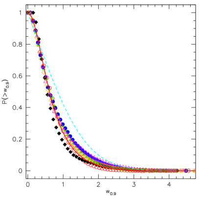
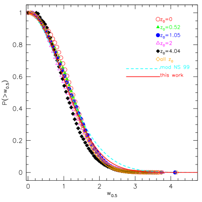
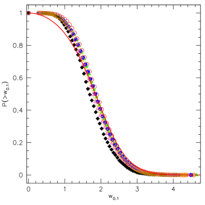
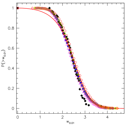
Figure 1: Dependence of rescaled formation time distribution $p(w_{f})$ on the required fraction $f$ of the final halo mass that must have been assembled. Different symbols show results for different redshifts $z_{0}$ at which the hosts were identified in the GIF2 simulation. The dashed curve shows equation (6), modified following Giocoli et al. (2007). The solid curve shows our equation (10).

2.1 Scaled units

In principle, the distribution $p_{f}(>z_{f}|M_{0},z_{0})$ depends on $f$, $M_{0}$ and $z_{0}$. However, the analytic solution for $f\geq 1/2$ is actually a function of the scaled variable

$$w_{f}=\dfrac{\delta_{c}(z_{f})-\delta_{c}(z_{0})}{\sqrt{S(fM_{0})-S(M_{0})}}\,,$$ (5)

where $\delta_{c}(z)$ is the initial overdensity required for spherical collapse at $z$, extrapolated using linear theory to the present time and $S(M)$ is the variance in the linear fluctuation field when smoothed with a top-hat filter of scale $R=\left(3M/4\pi\bar{\rho}\right)^{1/3}$, where $\bar{\rho}$ is the comoving density of the background. When $z_{f}$ is rescaled in this way, then the shape of $p(>w_{f}|M_{0},z_{0})$ is essentially the same for all values of $M_{0}$ and $z_{0}$, although the dependence on $f$ is still strong. E.g., for $f\geq 1/2$, the expected shape of this distribution is

$$p_{f}(w_{f})=\left(\dfrac{1}{f}-1\right)\mathrm{erfc}\left(\dfrac{w_{f}}{\sqrt{2}}\right)+\left(2-\frac{1}{f}\right)\sqrt{\dfrac{2}{\pi}}\mathrm{exp}\left(-\dfrac{w_{f}^{2}}{2}\right)\,$$ (6)

(Lacey & Cole, 1993; Nusser & Sheth, 1999). In what follows, we show that in our simulations this remains true for smaller values of $f$ as well. Recent work (Paranjape et al., 2011; Musso & Sheth, 2012) suggests that $w_{f}$ may not be the ideal choice for the scaling variable – this may account for some of the small departures from self-similarity that are evident in the following plots. This means that we do not need to fit a different functional form for each value of $f$, $M_{0}$ and $z_{0}$. Rather we need only fit to $p(w_{f})$, which is a function of $f$ and $w_{f}$ only. The expression above can become negative at $f<1/2$, so it is not a viable model for a probability distribution in this regime. Therefore, our main goal is to provide a fitting formula which works even at small $f$.

Although we can use this fitting formula for the full distribution $p(w_{f})$ to estimate the mean $\langle w_{f}\rangle$, we will be more interested in its median $\tilde{w_{f}}$. This is because the median formation redshift for fixed $f$ satisfies

$$\delta_{c}(z_{f})=\delta_{c}(z_{0})+\tilde{w_{f}}\,\sqrt{S(fM_{0})-S(M_{0})}$$ (7)

whereas the median main progenitor mass at fixed $z>z_{0}$ satisfies

$$S(\tilde{f}M_{0})=S(M_{0})+\frac{[\delta_{c}(z)-\delta_{c}(z_{0})]^{2}}{\tilde{w_{f}}^{2}}.$$ (8)

(Because both $S(fM_{0})$ and $\tilde{w_{f}}$ depend on $f$, this last expression must be solved to yield $\tilde{f}$.) In practice, these both trace out the same relation, so for the purposes of making plots, it suffices to rewrite the expression for the median formation redshift as:

$$\frac{\delta_{c}(z_{f})}{\delta_{c}(z_{0})}=1+\tilde{w_{f}}\,\sqrt{\frac{S(M_{0})}{\delta^{2}_{c}(z_{0})}}\,\sqrt{\frac{S(fM_{0})}{S(M_{0})}-1}\,.$$ (9)

To an excellent approximation, the left hand side is just the ratio of linear theory growth factors at the two redshifts. E.g., for an Einstein-de Sitter model (itself an excellent approximation for redshifts greater than about 2), this ratio would be $(a_{0}/a_{f})=(t_{0}/t_{f})^{2/3}$. And, for a power-law spectrum the final term on the right hand side is just a function of $f$. Since $\tilde{w_{f}}$ is also a function of $f$ only, the only mass dependence comes from $S(M_{0})/\delta^{2}_{c}(z_{0})$. If we fix the mass, then this term decreases as $z_{0}$ increases, so the distribution of $(t_{f}/t_{0})$ is expected to shift towards unity as the redshift at which the halos are identified increases.

3 A fitting formula for the formation time distribution

In what follows, we will use the GIF2 numerical simulation (Gao et al., 2004; Giocoli et al., 2008) to calibrate our fitting formula for $p_{f}(w_{f})$.

3.1 The simulation

The GIF2 simulation data we analyze below are publicly available at http://www.mpa-garching.mpg.de/Virgo. The simulation itself is described in some detail by Gao et al. (2004). It represents a flat $\mathrm{\Lambda}$ cold dark matter ($\mathrm{\Lambda}$CDM) universe with parameters ($\Omega_{m}$, $\sigma_{8}$, $h$, $\Omega_{b}h^{2}$ ) = ($0.3$, $0.9$, $0.7$, $0.0196$). The initial density fluctuation spectrum had an index $n=1$, with transfer function produced by cmbfast (Seljak & Zaldarriaga, 1996). The simulation followed the evolution of $400^{3}$ particles in a periodic cube $110\,\mathrm{Mpc}/h$ on a side. The individual particle mass is $1.73\times 10^{9}\,M_{\odot}/h$, allowing us to study the formation histories of a large sample of haloes spanning a wide mass range. Particle positions and velocities were stored at 53 output times, mainly logarithmically spaced between $1+z=20$ and $1$. Halo and subhalo merger trees were constructed from these outputs as described by Tormen et al. (2004); Giocoli et al. (2007, 2008).

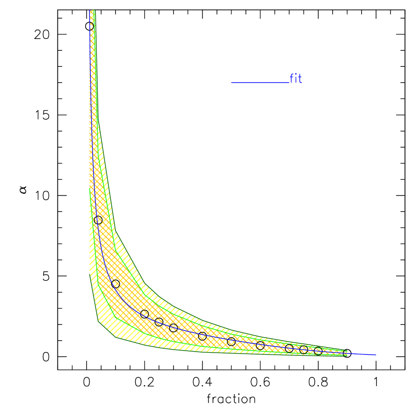
Figure 2: Dependence of $\alpha_{f}$, the free parameter in equation (10), on the mass fraction $f=m_{\rm MP}/M_{0}$ required for formation.

At each simulation snapshot haloes were identified using a spherical overdensity criterium. At each snapshot the density of each particle is assumed to be inversely proportional to the cube of the distance to the tenth nearest neighbor. We take as centre of the first halo the position of the densest particle. We then grow a sphere of matter around this centre, and stop when the mean density within the sphere falls below the virial value appropriate for the cosmological model at that redshift; we used the fitting formulae of Eke et al. (1996) for the virial density. All the particles inside this sphere are assigned to the new forming halo and are removed from the list. Starting from the second densest available particle we build the second halo, and so on until all the particles have been scanned. Particles not assigned to any collapsed objects are defined as field particles.

For each halo more massive than $10^{11.5}\,M_{\odot}/h$ (i.e. containing at least $\sim 200$ particles) in the five snapshots, corresponding to $z_{0}=0$, $0.52$, $1.05$, $2$ and $4.04$ we build up the merger history tree as follows. Starting from a halo at $z=z_{0}$, we define its progenitors at the previous output, $z=z_{0}+\mathrm{d}z_{1}$, as all haloes containing at least one particle that at $z=z_{0}$ will belong to that halo. The “main progenitor” at $z_{0}+\mathrm{d}z_{1}$ is defined as the one which provides the most mass to the halo at $z_{0}$. Then we repeat the same procedure, now starting with the main progenitor at $z=z_{0}+\mathrm{d}z_{1}$ and identify its main progenitor at $z=z_{0}+\mathrm{d}z_{1}+\mathrm{d}z_{2}$, and so on backward in time. Since we always follow the main progenitor halo, the resulting merger tree consists of a main trunk, which traces the main progenitor back in time, $m_{\rm MP}(z)$, and of “satellites”, which are all the progenitors which, at any time, merge directly onto the main progenitor.

In what follows, to guarantee a well-defined sample of relaxed haloes, we excluded all halos for which $m_{\rm MP}(z)$ exceeded the final host halo mass by more than $10\%$, as well as all halos which were, in fact, unbound.

3.2 The fitting formula

Figure 1 shows the cumulative distribution of rescaled formation redshifts. Each panel shows results for a different value of $f$, as indicated in the axis labels $f=0.9,0.5,0.1$ and $0.01$. In each panel, symbols show the measurements for haloes more massive than $10^{11.5}\,h^{-1}M_{\odot}$ identified at five different redshifts, approximately $z_{0}=0,1/2,1,2,$ and 4. Clearly, scaling $z_{f}$ to $w_{f}$ produces curves which are approximately independent of redshift.

The solid line shows the result of fitting

$$P(>w_{f})=\frac{\alpha_{f}}{\mathrm{e}^{w_{f}^{2}/2}+\alpha_{f}-1}$$ (10)

to the measurements. This returns a value $\alpha_{f}$ for each $f$, which is shown by the symbols in Figure 2. The $\alpha_{f}(f)$ relation is well described by

$$\alpha_{f}=0.815\,\mathrm{e}^{-2f^{3}}/f^{0.707}\,,$$ (11)

which is shown as the solid curve in each panel. The shaded regions around each curve show the 1 and 2$\sigma$ contours of $\Delta\chi^{2}$, where $\chi^{2}(\alpha_{f})=\sum_{i}[P_{i}-P(>w_{i,f},\alpha_{f})^{2}]$, is computed for each mass and redshift bin. (Equation 10 continues to provide a good fit if we define formation using $m_{1}$ rather than $m_{\rm MP}$, with the only difference being that $\alpha_{f}=0.867\,\mathrm{e}^{-2f^{3}}/f^{0.8}$. This $\alpha_{f}$ is larger than that for $m_{\rm MP}$ by a factor of $1.06/f^{0.1}$: the median $w_{f}$ is shifted to higher redshifts than when formation is defined using the main progenitor.)

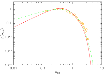
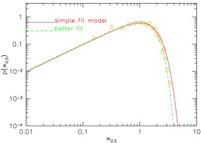
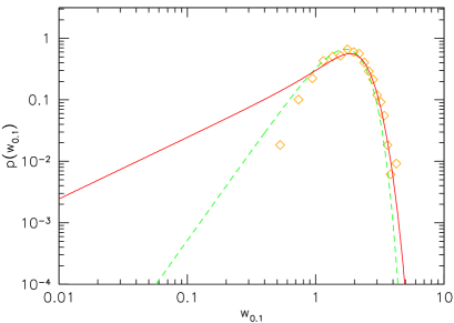
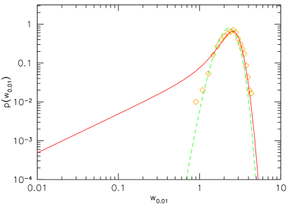
Figure 3: Differential formation time distribution. Open diamonds show the results from the GIF2 simulation for haloes more massive than $10^{11.5}\,h^{-1}M_{\odot}$ identified at five redshifts $z_{0}=0$, $0.52$, $1.05$, $2$ and $4.04$. The solid and dashed curves show the result of fitting to equations (12) and (15).

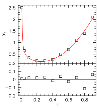
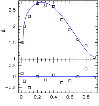
Figure 4: Dependence of the best-fit free parameters in equation (15) on $f$; curves show the scalings given by equations (17) and (18). The bottom panels show the residuals from these relations.

Figure 1 shows that equation (10) is reasonably accurate at least between the first and third quartiles of the distributions. The associated differential distribution is

$$p(w_{f})=-\dfrac{\partial P(>w_{f})}{\partial w_{f}}=-\dfrac{\alpha_{f}w\mathrm{e}^{w^{2}/2}}{\left[\mathrm{e}^{w^{2}/2}+\alpha_{f}-1\right]^{2}}.$$ (12)

It has median

$$\tilde{w_{f}}=\sqrt{2\,\ln\left(\alpha_{f}+1\right)}\,.$$ (13)

and the mean, computed via equation (4), is

$$\langle w_{f}\rangle=\sqrt{\pi/2}\,\frac{\alpha_{f}}{1-\alpha_{f}}\,\sum_{k=1}^{\infty}\frac{(1-\alpha_{f})^{k}}{k^{1/2}}.$$ (14)

For large values of $f$, $\alpha_{f}\ll 1$, and $\langle w_{f}\rangle\to\sqrt{\alpha_{f}\pi^{2}/2}$ whereas $\tilde{w_{f}}\to(2/\pi)\langle w_{f}\rangle$. In this limit, the distribution is rather skewed. However, it becomes less skewed as $f$ increases. When $\alpha_{f}=1$, then $\langle w_{f}\rangle=\sqrt{\pi/2}=1.25$ whereas $\tilde{w_{f}}=\sqrt{2\,\ln(2)}=1.18$. And when $f=0.04$ then $\alpha_{f}=8$ so $\langle w_{f}\rangle=2.06$ whereas $\tilde{w_{f}}=2.09$.

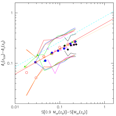
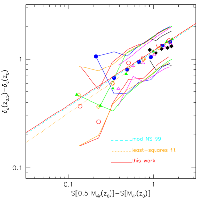
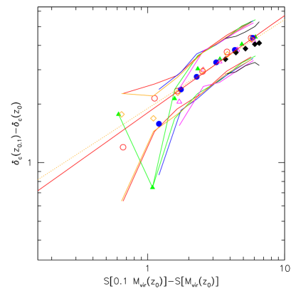
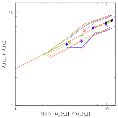
Figure 5: Correlation between formation redshift – defined as the first time that the main progenitor contains a fraction $f$ of the final mass $M_{0}$ – and host halo mass, expressed in scaled units. The different panels show results for different choices of $f$ (same as previous figure). The symbols, also same as previous figure, show results for different $z_{0}$. The dotted, dashed, and solid lines show a least-squares to the data at all redshifts (open diamonds), the relation associated with equation (6), and the prediction of our simple model (equation 13). In this format, both models predict a line of slope 1/2, so they only differ in the value of the zero-point.

Since equation (12) is not very accurate in the tails of the distribution, we have also fit $p(w_{f})$ to

$$p(w_{f})=A_{0}\,w_{f}^{0.63f^{-2/3}}\,\mathrm{e}^{-\gamma_{f}w_{f}^{\beta_{f}}}\,$$ (15)

where $A_{0}=\beta\,\gamma_{f}^{B_{0}}/\Gamma(B_{0})$ is a normalization factor, with $B_{0}=(1+0.63f^{-2/3})/\beta_{f}$. For this model the mean is

$$\langle w_{f}\rangle=\int dw_{f}\,p(w_{f})\,w_{f}=\gamma_{f}\,\frac{\Gamma(B_{0}+1/\beta_{f})}{\Gamma(B_{0})}$$ (16)

but one must estimate the median numerically.

Figure 3 compares the differential formation redshift distribution for four values of the assembled fraction $f$, with our two fitting functions. The symbols show the measurements for haloes more massive than $10^{11.5}\,h^{-1}M_{\odot}$ at five different $z_{0}$, as in Figure 1. For equation (15) (dashed curves), the best-fit parameters $\gamma_{f}$ and $\beta$ satisfy

$$\gamma_{f}=0.12+\dfrac{1}{290\,f^{1.4}}+4.3(f-0.24)^{2}\,,$$ (17)

and

$$\beta_{f}=3.05\,\mathrm{e}^{-0.6\gamma_{f}}+\dfrac{\mathrm{e}^{3.2\gamma_{f}}}{3800}\,.$$ (18)

Figure 4 shows these scalings. Despite the fact that equation (15) provides a more accurate description of the measurements, we have found equation (12) to be more useful because it comes with a simple expression for the median relation.

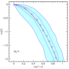
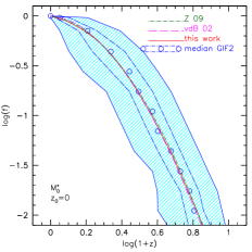
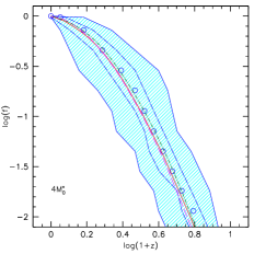
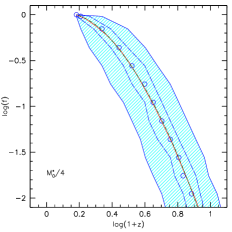
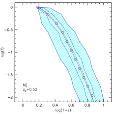
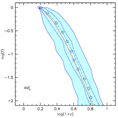
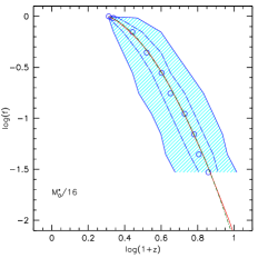
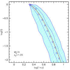
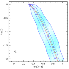
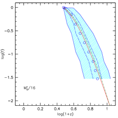
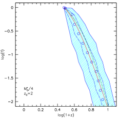
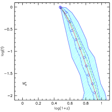
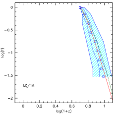
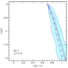
Figure 6: Mass growth history of dark matter haloes in the $\mathrm{\Lambda CDM}$ GIF2 cosmology. The different panels refer to various redshifts and host halo masses, as labeled. In each panel, open circles show the median $z$ at fixed $m/M$, and the curves that enclose them show the first and the third quartiles of the distribution defined by the GIF2 sample. These curves are the same as those for the median $m/M$ at fixed $z$: as expected from equation (2). The dot-dashed, dashed and solid curves show the model of Zhao et al. (2009), van den Bosch (2002) (valid only for haloes starting from $z_{0}=0$) and our equation (9).

3.3 Test of scaled units

Figure 5 shows the correlation between the formation redshift (for $f=0.9$, $0.5$, $0.1$ and $0.01$) and the host halo mass for the same choices of $z_{0}$ as before, in scaled units. I.e., the redshift is expressed as $\delta_{c}(z_{f})-\delta_{c}(z_{0})$ and the mass as $S(fM_{0})-S(M_{0})$. The different symbols represent different $z_{0}$ (same as Figure 1); they show the median of the correlation, i.e., the median of $\delta_{c}(z_{f})-\delta_{c}(z_{0})$ in bins of $S(fM_{0})-S(M_{0})$, while the solid lines of the same color show the first and third quartiles. The dotted and solid lines in each panel show a least-squares fit to the correlation, and the prediction of our model (equation 13). The dashed line in the two top panels shows the prediction, $N(>m,z_{f}|M_{0},z_{0})=1/2$, associated with equation (6). Note that, in the format we have chosen to present our results, the prediction boils down to a line of slope 1/2, with zero-point equal to $\log_{10}\tilde{w}_{f}$.

3.4 The median mass accretion history

As described above, we have obtained the merger history tree for each halo more massive than $10^{11.5}\,h^{-1}M_{\odot}$ at $z_{0}$, for four different choices of $z_{0}$. Figure 6 shows the mass of the main halo progenitor, in units of the mass at $z_{0}$, as a function of $z$. The different panels show results for parent halos of different masses, here expressed as fractions of $M^{*}_{0}$ (where $S(M^{*}_{0})\equiv\delta^{2}_{c}(0)$, so $M^{*}_{0}$ corresponds to $8.9\times 10^{12}\,M_{\odot}/h$). From top to bottom we show the halo accretion histories starting from different redshifts $z_{0}$. The open circles and dashed curve which enclose them represent the median, the first and the third quartile of the tree extracted from the simulation. The solid curves enclose $95\%$ of the trees.

Equation (2) shows that, for these median quantities, it should not matter if we plot the median $z_{f}$ at fixed $m/M=f$, or the median $f$ at fixed $z$. This is indeed the case, and is in contrast to what would have happened if we had chosen to show the corresponding mean values: the curve which traces $\langle z_{f}|f\rangle$ as a function of $f$ is slightly different from that which traces $\langle f|z_{f}\rangle$ as a function of $z$. Our equation (2) shows that this is a consequence of the mean not being the same as the median: the distributions are skewed.

The dot-dashed curve in each panel shows the prediction of Zhao et al. (2009): it describes our measurements very well. The dashed curve (for $z_{0}=0$ only), shows the model of van den Bosch (2002). The solid curve in each panel shows our model, evaluated as follows: given $M_{0}$ at redshift $z_{0}$, we compute $S(M_{0})$, $\delta_{c}(z_{0})$, and a table of $S(f\,M_{0})$ for any $0<f<1$. Inverting equation (13) then gives $z_{f}$ via equation (9). This agrees very well with the numerical simulation results and therefore also with the model of Zhao et al. (2009). But note that our prescription is much easier to implement.

3.5 Correlation between formation times

So far, we have mainly tested if $w_{f}$ is indeed a good scaling variable for the entire range of $f$. In what follows, it is interesting to know if the different formation time definitions are correlated. E.g., if a halo is above the median formation redshift for one value of $f$, is it also likely to have formed at above average $w_{f}$ for another $f$? Figure 7 shows that this correlation is weak, at least for $f=1/2$ and 0.04: When $w_{0.5}-\langle w_{0.5}\rangle$ and $w_{0.04}-\langle w_{0.04}\rangle$ are normalized by their rms values, then the correlation coefficient is $\sim 0.25$.

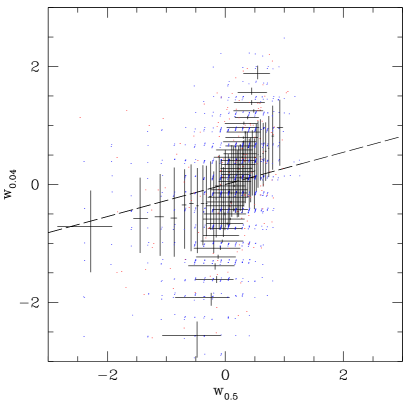
Figure 7: Correlation between formation times, when formation is defined as the first time that the main progenitor $m_{\rm MP}$ contains 0.5 and 0.04 of the total mass. We have scaled the variables by their rms values, so the fact that the median $w_{0.5}/\sigma_{0.5}$ at fixed $w_{0.04}/\sigma_{0.04}$ is rather different from the median $w_{0.04}/\sigma_{0.04}$ at fixed $w_{0.5}/\sigma_{0.5}$ indicates that the correlation between these two is weak.

3.6 Halo concentrations from masses and formation times

Equation (1) states that the formation time $t_{0.04}$ of a halo can be converted into an estimate of its concentration. To check this, we estimated $c_{vir}$ for each halo in GIF2 by fitting the matter density profile to the NFW functional form,

$$\rho(r|M_{vir})=\frac{\rho_{s}}{r/r_{s}(1+r/r_{s})^{2}}\,,$$ (19)

where

$$\rho_{s}=\frac{M_{vir}}{4\pi(R_{vir}/c_{vir})^{3}}\left[\ln(1+c_{vir})-\frac{c_{vir}}{1+c_{vir}}\right]^{-1}\,$$ (20)

and $c_{vir}\equiv r_{s}/R_{vir}$. Figure 8 shows the correlation between $c_{vir}$ and $t_{0}/t_{0.04}$, for various $M_{vir}$ and $z_{0}$. The dot-dashed curve (same in each panel) shows equation( 1): if $c_{vir}$ were completely predicted by $t_{0}/t_{0.04}$ then there should be no scatter around this relation.

In each panel, dots show the halos, and triangles with error bars show the median and first and third quartiles in ${\rm log}_{10}(c_{vir})$ for narrow bins in $t_{0}/t_{0.04}$. The actual distributions of $\log_{10}(c_{vir})$ and $\log_{10}(t_{0}/t_{0.04})$ are shown along the left axis and across the bottom. (Note that, for each $M_{0}$ bin, the peak of the distribution of $t_{0}/t_{0.04}$ shifts towards unity as $z_{0}$ increases, for the reason given following equation 9.) Clearly, although equation (1) provides a reasonable description of the triangles, the scatter around this relation is considerable. Quantitatively, the scatter in $\log_{10}c_{vir}$ is $0.13$ dex for $z_{0}=0$ halos with $M_{vir}\geq 10^{13}h^{-1}M_{\odot}$.

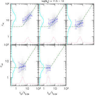
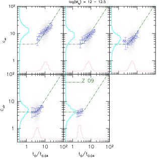
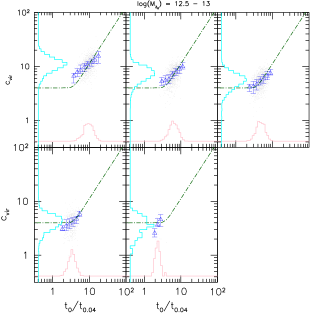
Figure 8: Correlation between host halo concentration and the time at which the system assembled $4\%$ of its mass. The different panels (left, central and right) show results for different host halo masses $M_{0}$, while the different windows show results for different $z_{0}$ (same as Figure 9). The histograms show the distributions of $c_{vir}$ and $t_{0}/t_{0.04}$, and the symbols with error bars show the correlation between them: the median and first and third quartiles of the distribution of $c_{vir}$ at each $t_{0}/t_{0.04}$. The dot-dashed curve shows equation (1).

The previous subsection showed that $t_{0.5}$ and $t_{0.04}$ of a halo are only weakly correlated. So it is reasonable to ask if some of the scatter in $c_{vir}$ can be removed if one includes information about $t_{0.5}$. E.g., one might reasonably expect the most concentrated halos to have small values of both $t_{0.5}$ and $t_{0.04}$. We have found that the typical concentration scales as

$$\log_{10}c_{vir}=\log_{10}0.45\,\left[4.23+\left(\frac{t_{1}}{t_{0.04}}\right)^{1.15}+\left(\frac{t_{1}}{t_{0.5}}\right)^{2.3}\right].$$ (21)

For halos more massive than $10^{13}h^{-1}M_{\odot}$, the rms scatter around this relation (0.1 dex) is indeed reduced with respect to the case in which only $t_{0.04}$ is known (0.12 dex). Evidently, the remaining scatter is due to other processes. Table 1 summarizes how this scatter decreases as more information is added.

Table 1: Precision of concentration estimates for halos with $M_{vir}>10^{13}\,h^{-1}M_{\odot}$.

rms$(\log_{10}c_{vir}|M_{vir})$	$0.124$
rms$(\log_{10}c_{vir}|\tau_{0.04},M_{vir})$	$0.120$
rms$(\log_{10}c_{vir}|\tau_{0.5},\tau_{0.04},M_{vir})$	$0.100$

One of the main goals of this paper is to provide a simple algorithm for generating the $M-c$ relation. Figure 9 shows this relation in GIF2. The open circles show the median of the distribution at fixed mass, and the error bar encloses the first and third quartiles. Different panels show results for different redshifts. The dotted line shows a least-squares fit to the data, while the dot-dashed and solid curves show the relations which come from inserting the mass accretion histories of Zhao et al. (2009) and our equation (9) into equation (1). Both approaches capture the mass dependence of the concentration, and its flattening with redshift, very well. But note that our estimate of the value of $t_{0.04}/t_{1}$ that is appropriate for a given mass bin (e.g., our equation 9), is much more straightforward to implement.

The $M-c$ relation for masses of order $10^{6}M_{\odot}$ is needed for modeling the milli-lensing effects of galaxy-size halo substructures (Keeton, 2003; Keeton et al., 2003; Sluse et al., 2003; Metcalf & Madau, 2001; Metcalf & Amara, 2012). The small mass regime is also important for estimating the dark matter annihilation signal coming from the integrated effect of substructures and field haloes at masses smaller than $10^{6}M_{\odot}$ (Pieri et al., 2005; Giocoli et al., 2008; Giocoli et al., 2009). However, this is below the mass resolution of current numerical simulations. Therefore, Figure 10 shows the result of using our model (equation (9, where $t_{0.5}$ and $t_{0.04}$ are obtained using our mass accretion history model) to estimate the $M-c$ relation at six different redshifts down to $3\times 10^{4}h^{-1}M_{\odot}$.

3.7 Formation times from masses and concentrations

In real datasets, while we may hope to have a reasonable estimate of the mass of the host halo, and perhaps of its concentration, we are unlikely to know either $t_{0.04}$ or $t_{0.5}$. So one might reasonably ask how well $t_{f}$ can be predicted given knowledge of either $M_{vir}$, $c_{vir}$ or both.

Table 2: Precision of formation time estimates for halos with $M_{vir}>10^{13}\,h^{-1}M_{\odot}$.

rms$(\tau_{0.5}|M_{vir})$	$0.123$
rms$(\tau_{0.5}|c_{vir})$	$0.088$
rms$(\tau_{0.5}|c_{vir},M_{vir})$	$0.087$
rms$(\tau_{0.04}|M_{vir})$	$0.176$
rms$(\tau_{0.04}|c_{vir})$	$0.111$
rms$(\tau_{0.04}|c_{vir},M_{vir})$	$0.109$

^⋆ $\tau_{f}\equiv\log_{10}(t_{f}/t_{1})$

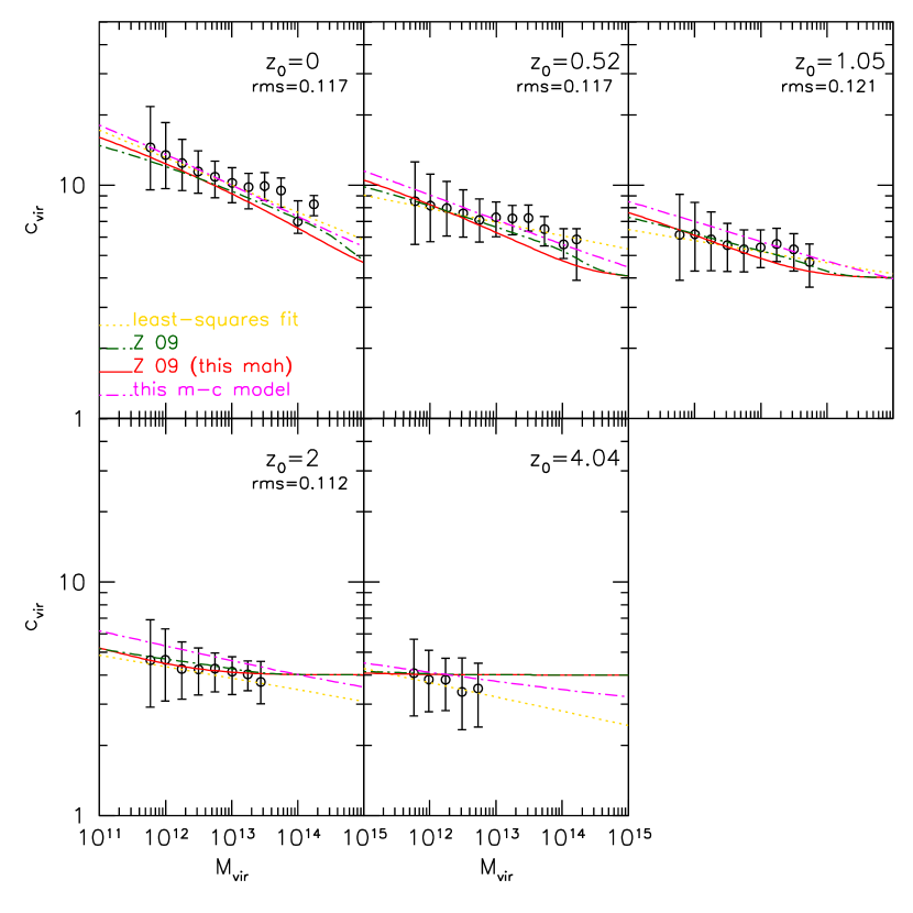
Figure 9: Median mass concentration relation in the GIF2 simulation. Open circles show haloes in the simulation at five different redshifts $z_{0}$, as labeled in the panels. Error bars show the first and the third quartiles of the distribution for each mass bin. The dotted line shows a least-squares fit to the data; dot-dashed and the solid curves show the predictions based on the median mass growth history of Zhao et al. (2009) and our equation (9). In each panel we show the rms in $\log_{10}(c_{vir})$ at fixed mass, for haloes more massive than $10^{13}\,M_{\odot}/h$.

Since equation (10) gives the distribution of $z_{f}$ given $M_{vir}$ and $z_{0}$, it can be manipulated to give the distribution of $t_{f}/t_{1}$ at fixed $M_{vir}$. In practice, we can get a good idea of the rms scatter around the mean by estimating how far on either side of the median value one must go before 68% of the total probability has been enclosed. These correspond to values of $w_{f}=\sqrt{2\ln(1+0.188\,\alpha_{f})}$ and $w_{f}=\sqrt{2\ln(1+5.303\,\alpha_{f})}$. For $f=0.04$ we have $\alpha_{f}=8$ so $w_{f}=1.35$ and $2.75$ respectively. For $M_{0}=8.9\times 10^{12}h^{-1}M_{\odot}$, $S(M_{0})/\delta_{c}^{2}(z_{0})=1$, so $\delta_{c}(z_{f})/\delta_{c}(z_{0})=2.81$ and 4.68, making $(t_{f}/t_{0})=0.18$ and $0.08$. Thus, the rms value of $\log(t_{f}/t_{0})$ should be about 0.16 dex. This is indeed close to the value 0.17 dex measured directly in the simulations. A similar analyis for $f=0.5$ returns similarly good agreement.

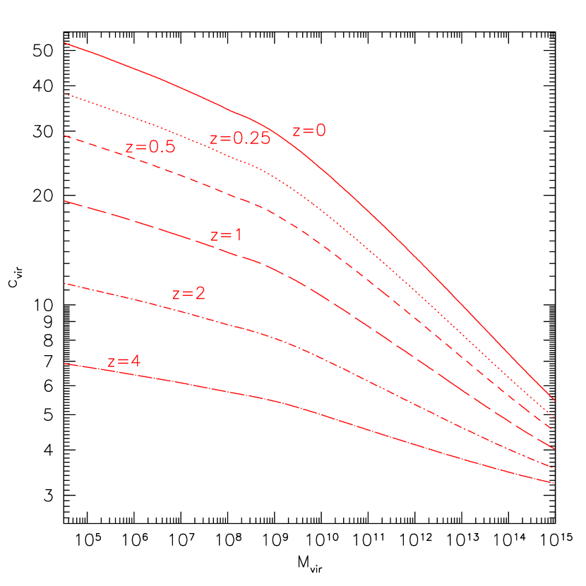
Figure 10: Mass concentration relation at six different redshifts predicted using equation (9). The concentration prediction has been extended down to small masses: $3\times 10^{4}M_{\odot}/h$.

The $t_{f}-c_{vir}$ relation is more complicated. If we define $\tau_{f}\equiv\log_{10}(t_{f}/t_{0})$, then at any $z_{0}$, $\langle\tau_{0.5}|c_{vir}\rangle\approx 0.175-0.503\log_{10}c_{vir}$ whereas $\langle\tau_{0.04}|c_{vir}\rangle\approx-0.049-0.825\log_{10}c_{vir}$. In both cases, the rms scatter around the fit is about 0.1 dex. Adding the mass does not reduce the scatter significantly, so we do not report fits to this case. Table 2 summarizes the precision with which a halo’s formation time can be predicted from its mass and concentration. In Figure 11 we show the correlation between the halo concentration and $\tau_{f}$, where $f=0.5$ on the left and $f=0.04$ on the right panel, for haloes with $M_{vir}\geq 10^{13}\,M_{\odot}/h$ and at any considered $z_{0}$. The data points with error bars show the median, with the quartiles, of both the concentration at fixed $t_{f}$ and vice versa. The solid lines show the leas-squares fit to the simulation data in both axsis.

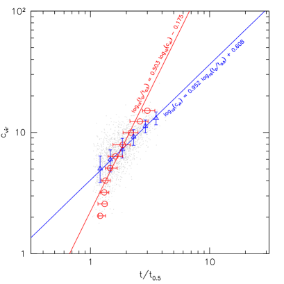
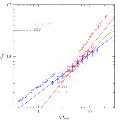
Figure 11: Correlation between concentration and $\tau_{f}$ ($f=0.5$ on the left and $f=0.04$ on the right panel). The data show simulation measurements at any $z_{0}$ for all haloes more massive than $10^{13}\,M_{\odot}/h$. Open triangles and circles show the median with the quartiles of respectively $c_{vir}$ at fixed $\tau_{f}$ and vice versa. The solid lines represent the least-squares fit to the simulation data points in both axsis.

4 Monte-Carlo realizations of mass accretion histories

We have used the distribution of formation times discussed above to generate Monte Carlo realizations of mass accretion histories as follows. In reality, $m_{\rm MP}$ changes continuously; the amount by which it changes at any given time is a random variable that is different for each halo. Most merger tree algorithms approximate this by taking (typically small) discrete steps in redshift, and then allow the mass to vary stochastically (Nusser & Sheth, 1999, e.g.); others allow large steps in time (Moreno et al., 2009). Our approach is rather different: we predetermine discrete steps in mass, and at each step, we draw a redshift from $p_{\rm MP}$ for that mass.

The choice of mass-step is critical. Two steps in mass $f_{1}M_{0}$ and $f_{2}M_{0}$ (with $f_{1}>f_{2}$) would be strongly correlated if $f_{1}\sim f_{2}$, but mass scales separated by $\Delta f/f\sim 1$ are approximately uncorrelated (Peacock & Heavens, 1990; Paranjape et al., 2011). Figure 7 shows that, at least for large $\Delta f/f$, the distributions are indeed reasonably independent.

We have found that if we set $\Delta\log_{10}M\approx-0.3$ then the distributions $p(w_{f_{1}})$ and $p(w_{f_{2}})$, when expressed as functions of redshift, do not overlap much. Since this mass difference corresponds approximately to $\Delta f/f\sim 0.5$, we assume that we can take independent picks from these redshift distributions, with the condition that for the small fraction of picks where $z_{2}<z_{1}$ occurs we should set $z_{2}=z_{1}$. If there were no overlap at all, our approach would correspond to having independent jumps in redshift, always having the correct distribution of redshifts at the predetermined discrete mass scales. Figure 12 shows the results. The filled triangles and the dashed curve that encloses them indicate the median and the first and third quartiles, solid curves enclose $95\%$ of the trees. The solid line shows our analytical prediction (equation 9).

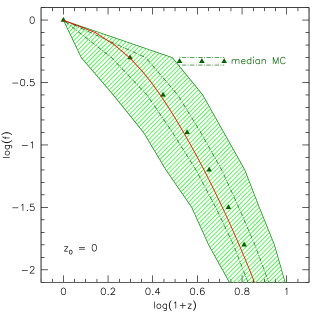
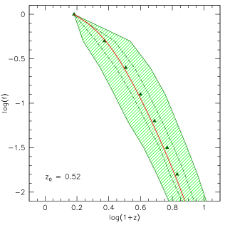
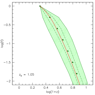
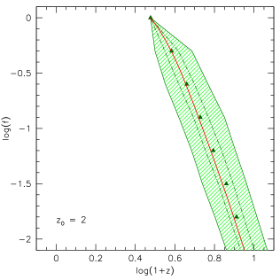
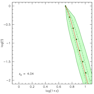
Figure 12: Mass growth history of a sample of $M_{0}^{*}$ haloes starting from different redshifts $z_{0}$. The sample as been built sampling a discrete number of mass steps with $\Delta\log_{10}M=-0.3$ for the rescaled formation redshit distributions between $z_{0}$ and $z>z_{0}$. The filled triangles and the curves that enclose them indicate the median and the first and the third quartiles. The solid line is our mass growth history model (equation 9).

5 Applications

Extended-Press & Schechter (1974) approach gives the possibility of estimating the main halo growth as function of the growth factor, the mass variance and the overdensity threshold for collapse. Once fixed the cosmological model these quantities can be translated in mass, redshift and time. For this reason the halo formation, growth and concentration depend on the cosmological parameters adopted (Harker et al., 2006; Power et al., 2011). In the left panel of the Figure 13 we show how much the median redshift of haloes at the present time, with $z_{0}$=0, differs with respect to a reference model in assembling $90\%$, $50\%$, $10\%$ and $1\%$ of their mass. We have compared $\sigma_{8}=0.8$ (bottom) and $\sigma_{8}=1$ (top) with respect to $\sigma_{8}=0.9$. $\sigma_{8}$ represents the amplitude of the linear power spectrum on a scale of $8$ Mcp$/h$, from the figure we notice that universes with a lower value of $\sigma_{8}$ tend to form haloes more recently. The same is valid if we consider the dark energy equation of state parameter $w$. In the right panel of Figure 13 we show the relative change in formation redshifts between $w=-1.1$ and $w=-0.9$ with respect to $w=-1$.

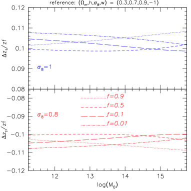
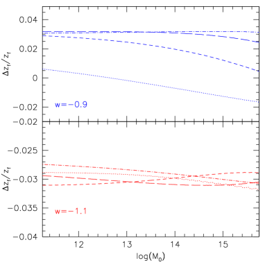
Figure 13: Correlation between the formation redshift and the virial host halo mass at $z_{0}=0$, for different choices of the mass fraction required for formation ($f=0.9$, $0.5$ $0.1$ and $0.01$). Left panel shows the relative change in formation redshift (and so the main halo growth and the halo abundance) for $\sigma_{8}=0.8$ and $\sigma_{8}=1$ relative to $\sigma_{8}=0.9$. Right panel shows the dependence on the equation of state parameter $w$.

Similarly to the previous figure, in Figure 14 we show the relative difference in formation redshifts in universes with lower and higher matter density parameter with respect to the model of the GIF2 simulation (we have assumed that $\Omega_{m}+\Omega_{\Lambda}=1$). In the same figure, the right panel quantify the change in formation redshift due to the change in Hubble constant.

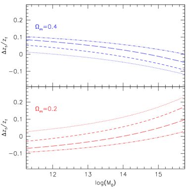
Figure 14: The same as Figure 13, in this case on the left we show the relative difference in formation redshifts for universes with lower and higher density parameter with respect to the GIF2 cosmology, the right with different Hubble constant.

From the figures above we notice that a bigger difference in formation redshifts can be mainly seen, for masses of the order of galaxy clusters, in universes with a different power spectrum normalization $\sigma_{8}$ and matter density parameter $\Omega_{m}$, a change of $0.1$ in $w$ and $h$ do not influence too much the formation time definitions.

6 Discussion and Conclusions

If the formation time of a halo is defined as the first time that its main progenitor exceeds a fraction $f$ of the final mass $M$, then, for halos of a given $M$, there will be distribution of formation times which depends on $f$. We argued that the median formation time as a function of $f$ should be the same as the median of $f$ as a function of time (equation 2), and showed that this was indeed the case (Figure 6).

We also argued that, to a good approximation, the distribution of formation times should be a function of the scaling variable $w_{f}$ defined in equation (5), even when $f<1/2$. The distribution of scaled formation times $p(w_{f})$ is indeed approximately independent of $M$ and $z_{0}$ (Figure 1). This distribution is well-described by equation (10). Its median has a simple form. When combined with a relation which relates formation time to halo concentration (equation 1), this provides a simple way to estimate the concentration of a halo. Including more information about the mass accretion history (e.g. equation 21) helps predict the concentration more precisely (Table 1).

We also studied how well a halo’s formation time could be predicted from knowledge of its mass and concentration. If the concentration is known, then the mass adds little new information about the formation time (Table 2). When the formation time is expressed in units of the time $t_{1}$ at which the halo was identified, then the concentration estimates $\log_{10}(t_{0.5}/t_{1})$ with rms 0.09 dex, and $\log_{10}(t_{0.04}/t_{1})$ with rms 0.11 dex. It may be that these scalings will find use in studies which compare the mean age of the stars in the central galaxy of a cluster with the time when the mass in the central core was first assembled.

The formation times for sufficiently different $f$ are only weakly correlated (Figure 7). We argued why this is not unexpected (Section 4) and then used this fact to devise a simple Monte-Carlo algorithm for generating mass accretion histories. The algorithm is rather accurate (Figure 12), and allows one to generate realistic mass accretion histories over a large range of masses and redshifts. We expect it to be useful for studies of how the $M-c$ relation depends on the background cosmological model. Algorithms for estimating the median main halo progenitor mass growth history and the concentration-mass relation are available here: http://cgiocoli.wordpress.com/research-interests/concentrationmah.

Appendix A Appendix

The main text defined halo formation using the main progenitor $m_{\rm MP}$, rather than the most massive progenitor $m_{1}$. In principle, predicting the distribution of $m_{1}(z)$, the most massive of the set of progenitors at $z$, is just an extreme value statistics problem. In practice, calculating this distribution is complicated by the fact that the partition of $M_{0}$ into $m_{1},\ldots,m_{n}$ does not involve $n$ independent picks from the same distribution. (E.g., for white-noise initial conditions, the joint distribution of the $n$ picks is known in closed form – see Sheth & Lemson (1999) – and it is not simply the product of $n$ identical distributions.) Similarly, there is no simple expression for the distribution of $m_{\rm MP}(z)$.

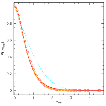
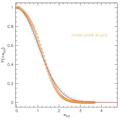
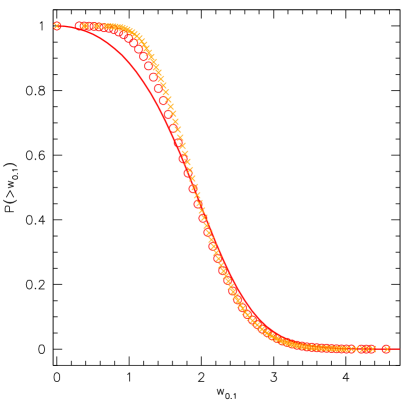
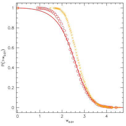
Figure 15: Distribution of scaled formation times for dark matter haloes identified at $z_{0}=0$, when formation is defined as the earliest time that $m_{\rm MP}\geq fM_{0}$ (circles) or as $m_{1}\geq fM_{0}$ (crosses) for different values of $f$. The solid curve shows our simple fitting function (equation 10) with $\alpha_{f}$ given by equation (22) rather than (11). Note that the two definitions coincide for $f\geq 1/2$, but that otherwise $m_{1}$ yields higher formation redshifts.

Figure 15 shows the cumulative formation time distribution of the sample of haloes identified at $z_{0}=0$. The open circles (same as Figure 1) show the measurements on the merger-tree where the main halo progenitor has been defined among the most contributing between two consecutive time steps, while for the crossed data we defined the main halo as the most contributing progenitor at $z_{0}=0$. The dashed and the solid curve are the same as in Figure 1 and represent our fit and the modified model by Nusser & Sheth (1999). As expected, the distributions are essentially identical when $f=0.9$ and $0.5$. However, at smaller values of $f$, the difference between the two definitions increases.

We can quantify this difference by noting that, if we fit equation (10) to this distribution, then the required scaling of $\alpha_{f}$ with $f$ becomes

$$\alpha_{f}=0.867\,\mathrm{e}^{-2f^{3}}/f^{0.8}\,.$$ (22)

Since this $\alpha_{f}$ is larger than that in the main text by a factor of $1.06/f^{0.1}$, equation (13) shows that the median $w_{f}$ is shifted to higher redshifts than when formation is defined using the main progenitor.

References

- Bullock et al. (2001) Bullock J. S., Kolatt T. S., Sigad Y., Somerville R. S., Kravtsov A. V., Klypin A. A., Primack J. R., Dekel A., 2001, MNRAS, 321, 559
- Dolag et al. (2004) Dolag K., Bartelmann M., Perrotta F., Baccigalupi C., Moscardini L., Meneghetti M., Tormen G., 2004, A&A, 416, 853
- Eke et al. (1996) Eke V. R., Cole S., Frenk C. S., 1996, MNRAS, 282, 263
- Eke et al. (2001) Eke V. R., Navarro J. F., Steinmetz M., 2001, ApJ, 554, 114
- Fu et al. (2008) Fu L., Semboloni E., Hoekstra H., Kilbinger M., van Waerbeke L., Tereno I., Mellier Y., Heymans C., Coupon J., Benabed K., Benjamin J., Bertin E., Doré O., Hudson M. J., Ilbert O., Maoli et al. 2008, A&A, 479, 9
- Gao et al. (2004) Gao L., White S. D. M., Jenkins A., Stoehr F., Springel V., 2004, MNRAS, 355, 819
- Giocoli et al. (2007) Giocoli C., Moreno J., Sheth R. K., Tormen G., 2007, MNRAS, 376, 977
- Giocoli et al. (2008) Giocoli C., Pieri L., Tormen G., 2008, MNRAS, 387, 689
- Giocoli et al. (2009) Giocoli C., Pieri L., Tormen G., Moreno J., 2009, MNRAS, 395, 1620
- Giocoli et al. (2010a) Giocoli C., Tormen G., Sheth R. K., van den Bosch F. C., 2010a, MNRAS, 404, 502
- Giocoli et al. (2008) Giocoli C., Tormen G., van den Bosch F. C., 2008, MNRAS, 386, 2135
- Harker et al. (2006) Harker G., Cole S., Helly J., Frenk C., Jenkins A., 2006, MNRAS, 367, 1039
- Keeton (2003) Keeton C. R., 2003, ApJ, 584, 664
- Keeton et al. (2003) Keeton C. R., Gaudi B. S., Petters A. O., 2003, ApJ, 598, 138
- Lacey & Cole (1993) Lacey C., Cole S., 1993, MNRAS, 262, 627
- Laureijs et al. (2011) Laureijs R., Amiaux J., Arduini S., Auguères J. ., Brinchmann J., Cole R., Cropper M., Dabin C., Duvet L., Ealet A., et al. 2011, ArXiv e-prints
- Macciò et al. (2008) Macciò A. V., Dutton A. A., van den Bosch F. C., 2008, MNRAS, 391, 1940
- Metcalf & Amara (2012) Metcalf R. B., Amara A., 2012, MNRAS, 419, 3414
- Metcalf & Madau (2001) Metcalf R. B., Madau P., 2001, MNRAS, 563, 9
- Moreno et al. (2009) Moreno J., Giocoli C., Sheth R. K., 2009, MNRAS, 397, 299
- Musso & Sheth (2012) Musso M., Sheth R. K., 2012, ArXiv e-prints
- Navarro et al. (1996) Navarro J. F., Frenk C. S., White S. D. M., 1996, ApJ, 462, 563
- Navarro et al. (1997) Navarro J. F., Frenk C. S., White S. D. M., 1997, ApJ, 490, 493
- Neto et al. (2007) Neto A. F., Gao L., Bett P., Cole S., Navarro J. F., Frenk C. S., White S. D. M., Springel V., Jenkins A., 2007, MNRAS, 381, 1450
- Nusser & Sheth (1999) Nusser A., Sheth R. K., 1999, MNRAS, 303, 685
- Paranjape et al. (2011) Paranjape A., Lam T. Y., Sheth R. K., 2011, MNRAS, p. 2019
- Peacock & Heavens (1990) Peacock J. A., Heavens A. F., 1990, MNRAS, 243, 133
- Pieri et al. (2005) Pieri L., Branchini E., Hofmann S., 2005, Physical Review Letters, 95, 211301
- Power et al. (2011) Power C., Knebe A., Knollmann S. R., 2011, MNRAS, p. 1734
- Prada et al. (2011) Prada F., Klypin A. A., Cuesta A. J., Betancort-Rijo J. E., Primack J., 2011, ArXiv e-prints
- Press & Schechter (1974) Press W. H., Schechter P., 1974, ApJ, 187, 425
- Schrabback et al. (2010) Schrabback T., Hartlap J., Joachimi B., Kilbinger M., Simon P., Benabed K., Bradač M., Eifler T., Erben et al. 2010, A&A, 516, A63+
- Seljak & Zaldarriaga (1996) Seljak U., Zaldarriaga M., 1996, ApJ, 469, 437
- Sheth et al. (2003) Sheth R. K., Bernardi M., Schechter P. L., Burles S., Eisenstein D. J., Finkbeiner D. P., Frieman J., Lupton R. H., Schlegel D. J., Subbarao M., Shimasaku K., Bahcall N. A., Brinkmann J., Ivezić Ž., 2003, ApJ, 594, 225
- Sheth & Lemson (1999) Sheth R. K., Lemson G., 1999, MNRAS, 305, 946
- Sluse et al. (2003) Sluse D., Surdej J., Claeskens J.-F., Hutsemékers D., Jean C., Courbin F., Nakos T., Billeres M., Khmil S. V., 2003, A&A, 406, L43
- Tormen et al. (2004) Tormen G., Moscardini L., Yoshida N., 2004, MNRAS, 350, 1397
- van den Bosch (2002) van den Bosch F. C., 2002, MNRAS, 331, 98
- Wechsler et al. (2002) Wechsler R. H., Bullock J. S., Primack J. R., Kravtsov A. V., Dekel A., 2002, ApJ, 568, 52
- Zhao et al. (2009) Zhao D. H., Jing Y. P., Mo H. J., Bnörner G., 2009, ApJ, 707, 354
- Zhao et al. (2003b) Zhao D. H., Jing Y. P., Mo H. J., Börner G., 2003b, ApJ, 597, L9