Vainshtein screening in a cosmological background in the most general second-order scalar-tensor theory
Abstract
A generic second-order scalar-tensor theory contains a nonlinear derivative self-interaction of the scalar degree of freedom à la Galileon models, which allows for the Vainshtein screening mechanism. We investigate this effect on subhorizon scales in a cosmological background, based on the most general second-order scalar-tensor theory. Our analysis takes into account all the relevant nonlinear terms and the effect of metric perturbations consistently. We derive an explicit form of Newton’s constant, which in general is time-dependent and hence is constrained from observations, as suggested earlier. It is argued that in the most general case the inverse-square law cannot be reproduced on the smallest scales. Some applications of our results are also presented.
pacs:
04.50.Kd, 95.36.+xI Introduction
Since the discovery of the accelerated expansion of the Universe SNe , numerous attempts have been proposed to explain the origin of this biggest mystery in modern cosmology. A vast class of models for cosmic acceleration invokes a scalar degree of freedom, , which may couple minimally or nonminimally to gravity and ordinary matter. In the case of nonminimal coupling, the models are commonly called modified gravity (or “dark gravity”) rather than dark energy, as participates in the long-range gravitational interactions and thereby accelerates the cosmic expansion. Modified gravity models must be designed with care, because otherwise the effect of modification could persist down to small scales, which could easily be inconsistent with stringent tests in the solar system and laboratories. For this reason, screening mechanisms for scalar-mediated force are crucial.
There are mainly two approaches for screening the scalar degree of freedom in modified gravity models. The first one is the Chameleon mechanism chameleon , by which the scalar acquires large mass in a high density environment. This is employed in viable gravity fr , which is equivalent to a scalar-tensor theory with an appropriate potential. The second one is the Vainshtein mechanism vainshtein . In this case ’s kinetic term becomes effectively large in the vicinity of matter due to some nonlinear derivative interaction, suppressing the effect of nonminimal coupling. The Vainshtein screening is typical in Galileon-like models gali1 and nonlinear massive gravity (e.g., nlmassive ). In the Vainshtein case, nonlinearities play an important role in possible recovery of usual gravity on small scales even in a weak gravity regime. To test models of modified gravity against experiments and cosmological observations, we therefore need to clarify the behavior of gravity around and below the scale at which the relevant nonlinearities set in. In this paper, we explore the consequences of the latter mechanism in detail, taking into account the nonlinear effect.
We study gravity sourced by a density perturbation of nonrelativistic matter, on subhorizon scales in a cosmological background, using the (quasi)static approximation. To provide generic results, we work in the most general scalar-tensor theory with second-order field equations Horndeski , which can be derived by generalizing the Galileon theory covg ; GenGal and therefore is expected to be endowed with the Vainshtein mechanism. In the context of the Galileon, previous works focus only on the scalar-field equation of motion to see the profile of (the gradient of) , ignoring gravity backreaction gali1 ; 5thforce .111In the course of the preparation of this manuscript, we became aware of the very recent paper by De Felice, Kase, and Tsujikawa recent , in which the metric under the influence of the Vainshtein mechanism is obtained for a static and spherically symmetric configuration in a subclass of the most general theory. Since our approach follows the cosmological perturbation theory on subhorizon scales koyama , the effect of metric perturbations can naturally be taken into account consistently. The results in this paper can be applied to various aspects of cosmology and astrophysics.
This paper is organized as follows. We define the theory we consider and then present the equations governing the background cosmological dynamics in the next section. In Sec. III we derive the perturbation equations with relevant nonlinear contributions using the subhorizon approximation. We then explore spherically symmetric solutions of the perturbation equations in Sec. IV. In Sec. V we present some simple applications of our results and finally we conclude in Sec. VI. In Appendix A, we summarize the definitions of coefficients in the equations in the main text. In Appendix B, we discuss a possible variety of solutions of the key equation (50). In Appendix C, we present the Fourier transform of the perturbation equations.
II Cosmology in the most general scalar-tensor theory
We consider a theory whose action is given by
| (1) |
where
| (2) | |||||
with four arbitrary functions, and , of and . Here stands for , and hereafter we will use such a notation without stating so. The Lagrangian is a mixture of the gravitational and scalar-field portions, as the Ricci scalar and the Einstein tensor are included. Note in particular that if a constant piece is present in then it gives rise to the Einstein-Hilbert term. We assume that matter, described by , is minimally coupled to gravity.
The Lagrangian (2) gives the most general scalar-tensor theory with second-order field equations in four dimensions. The most general theory was constructed for the first time by Horndeski Horndeski in a different form than (2), and later it was rediscovered by Deffayet et al. GenGal as a generalization of the Galileon. The equivalence of the two expressions is shown by the authors of Ref. G2 . In this paper, we employ the Galileon-like expression (2) since it is probably more useful than its original form when discussing the Vainshtein mechanism. The gravitational and scalar-field equations can be found in the Appendix of Ref. G2 .
We now replicate the cosmological background equations in the theory (1) G2 ; AKT . For and the background metric , the gravitational field equations are
| (3) | |||||
| (4) |
where
| (5) | |||||
| (6) | |||||
and is the (nonrelativistic) matter energy density, while the scalar-field equation of motion is
| (7) |
where
| (8) | |||||
| (9) | |||||
An overdot denotes differentiation with respect to and .
III Perturbations with relevant nonlinearities
We work in the Newtonian gauge, in which the perturbed metric is written as
| (10) |
with the perturbed scalar field and matter energy density,
| (11) | |||||
| (12) |
It will be convenient to use
| (13) |
which is dimensionless.
We wish to know the behavior of the gravitational and scalar fields on subhorizon scales sourced by a nonrelativistic matter overdensity . To do so, we may ignore time derivatives in the field equations, while keeping spatial derivatives. We assume that , , and are small, but nevertheless we do not neglect terms that are schematically written as and , where represents a spatial derivative and is any of , and . This is because could be larger than below certain scales, where is a typical length scale associated with which may be as large as the present Hubble radius. [As we will see, terms do not appear.]
The traceless part of the gravitational field equations is given by
| (14) |
where we defined a derivative operator
| (15) |
and
| (17) | |||||
| (18) | |||||
The coefficients such as , , , … that appear in the field equations here and hereafter are defined in Appendix A.
Applying the operator to the above quantities, we find
| (19) | |||||
| (20) | |||||
| (21) |
where . Thus, from the traceless equation (14) we obtain
| (22) |
The component of the gravitational field equations reads
| (23) | |||||
where
| (24) |
Finally, the equation of motion for reduces to
| (25) |
where
| (26) | |||||
Equations (22), (23), and (25), supplemented with the matter equations of motion (see Sec. V.1) govern the (quasi)static behavior of the gravitational potentials and the scalar field on subhorizon scales.
Note that in deriving Eqs. (23) and (25) we have neglected the “mass terms” and . These contributions could be larger than the higher spatial derivative terms, and in that case the fluctuation will not be excited. We do not consider this rather trivial situation and focus on the case where and can safely be ignored. Though restricted to the linear analysis, these terms have been considered in Ref. AKT .
Let us end this section with a short remark. One may notice that all the terms (except ) in Eqs. (22), (23), and (25) can be written as total divergences, as
Therefore, those equations can be integrated over a spatial domain , and then one is left with the boundary terms and the enclosed mass,
| (27) |
as a consequence of neglecting the “mass terms” mentioned above. This fact will be used explicitly in the next section.
IV Spherically symmetric configurations
We now want to consider a spherically symmetric overdensity on a cosmological background. For this purpose it is convenient to use the coordinate . We are primarily interested in scales much smaller than the horizon radius, . Under this circumstance the background metric may be written as , where is the line element of the unit two-sphere.
The spherical symmetry allows us to write
where a prime denotes differentiation with respect to . The gravitational field equations and scalar-field equation of motion can then be integrated once, leading to
| (28) | |||||
| (29) | |||||
where we defined
| (31) |
, and dimensionless coefficients
| (32) |
Note that is the propagation speed of gravitational waves which may be different from in general G2 . Note also that in deriving Eqs. (28)–(LABEL:eq3) we have set the integration constants to be zero, requiring that is a solution if .
For sufficiently large , we may neglect all the nonlinear terms in the above equations. The solution to the linear equations is given by
| (33) | |||||
| (34) | |||||
| (35) |
where we defined . In this regime, the parametrized post-Newtonian parameter is given by
| (36) |
which in general differs from unity.
IV.1
A simple example for which nonlinear terms can operate is the model with and , i.e.,
| (37) |
In this case, we have and . We also have the relation
| (38) |
The Lagrangian (37) corresponds to a nonminimally coupled version of kinetic gravity braiding KGB , and has been studied extensively in the context of inflation G-inf and dark energy/modified gravity GDE ; KY1 ; KY2 . Of course the nonminimal coupling can be undone by performing a conformal transformation, but in the present analysis we have no particular reason to do so. Note that even in the case of const the scalar is coupled to the curvature at the level of the field equation, which signals “braiding.”
Using Eqs. (28) and (29), Eq. (LABEL:eq3) reduces to a quadratic equation
| (39) |
where
| (40) |
Equation (39) can easily be solved to give
| (41) |
At short distances, , one finds
| (42) |
In order for this solution to be real, we require
| (43) |
In this regime, the metric potentials are given by
| (44) | |||||
| (45) |
where
| (46) |
If , the typical length scale can be estimated using Eq.(46) as
| (47) |
where .
Note that in this case the Friedmann equation can be written as
| (48) |
where and . Thus, the effective gravitational coupling governing short-distance gravity is the same as the one in the Friedmann equation.
The Vainshtein mechanism successfully screens the effect of the fluctuation , so that the two metric potentials coincide and exhibit the Newtonian behavior at leading order. However, is time-dependent since it is a function of the time-dependent field , which means that the Vainshtein mechanism cannot suppress the time variation of in a cosmological background. This fact was first noticed in Ref. Time-varying . We will discuss this point further in the next subsection.
IV.2
Let us consider a class of models with . In this case, we see that . For the other nonzero coefficients we have the following relations:
| (49) |
With , the problem reduces to solving a cubic equation one can handle. Indeed, using Eqs. (28) and (29) to remove and from Eq. (LABEL:eq3), we obtain the cubic equation for :
| (50) |
where -independent coefficients are defined as
| (51) |
We note the expressions for and in terms of :
| (52) |
Linearizing Eq. (50) at , one obtains the solution (35) as expected. This will be matched to one of the following three solutions at short distances:
| (53) |
If simply ,222This is probably the most natural case if one considers a model that accounts for the present cosmic acceleration and the coefficients are evaluated at present time, because in that case there is only one typical length scale . the two regimes are connected at around , where
| (54) |
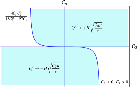
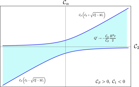
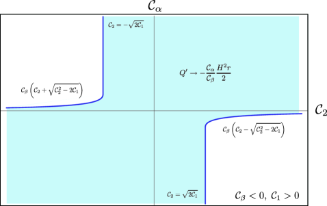
If and , the solution with the boundary condition (35) at large can be matched either to or to . We call this situation Case I. This is possible for in the shaded region in Fig. 1. For (respectively ), the short-distance solution is given by (respectively ). Outside this region one cannot find a solution that is real for . A typical behavior of the Case I solution is plotted in Fig. 2. If , then the solution can be matched only to . We call this situation Case II. This is possible for in the shaded region in Figs. 3 () and 4 (). Outside this region no real solutions can be found. If and then no real solutions can be found either.
Let us then evaluate the metric perturbations for each solution . We begin with the Case I, . The metric potentials at short distances are given by
| (55) |
where
| (56) | |||||
| (57) |
Although the coefficients look apparently different, now we use the relations (49) for the first time to show that
| (58) |
i.e., the two metric potentials actually coincide. We thus obtain the Newtonian behavior
| (59) |
It is interesting to note that the above conclusion holds even for the generic propagation speed of gravitational waves, . Explicitly, one finds
| (60) |
As in the case of the previous subsection, is in general time-dependent, as it is a function of time-dependent and . We thus illustrate how the Vainshtein mechanism fails to suppress the time variation of in a cosmological background within the context of some generic scalar-tensor theories minimally coupled to matter. The claim was originally suggested using the Einstein frame action in Ref. Time-varying . Here we explicitly give the concrete formula with which one can evaluate the time variation of for a given model.
If happens to vary very slowly, we can say that the usual Newtonian gravity is reproduced in the vicinity of the source. However, in general, one expects that varies on cosmological time scales. The time variation is constrained from lunar laser ranging experiments to be LLR .
At this stage it is interesting to look at the background evolution for the models with . The (modified) Friedmann equation (3) can be written as
| (61) |
where the gravitational coupling in the Friedmann equation read off from the above exactly coincides with the expression for ,
| (62) |
and
The situation here is the same as what we have seen in the previous subsection. We refer to a constraint in Ref. uzan , obtained by translating the big bang nucleosynthesis (BBN) bound on extra relativistic degrees of freedom, as
| (63) |
where (respectively, ) is evaluated at the time of BBN (respectively, today).
Having thus seen that the Newtonian behavior is reproduced with time-dependent , let us then evaluate leading order corrections to the potentials. In this case we need to keep the subleading term in :
| (64) |
From this we obtain the corrections and as
| (65) | |||
| (66) |
For the solution , we find
| (67) |
implying that the parametrized post-Newtonian parameter is given by . Therefore, is tightly constrained from solar-system tests in this case: Will .
When the coefficients , and have hierarchies in their values, we find a variety of solutions to Eq. (50) on an intermediate scale between the linear regime at large and the small limit of Case I or Case II. The details are summarized in Appendix B, which could be potentially confronted with observations.
IV.3
Let us finally discuss the most general case where all the coefficients in Eqs. (28)–(LABEL:eq3) are nonzero. Although one can still eliminate and to get an equation solely in terms of , the resulting equation will be a sextic equation. This hinders us from analyzing a variety of possible solutions in detail. However, for and one can show that there is no solution such that on sufficiently small scales. To show this, one substitutes to Eq. (28). The second term in the right-hand side can be compensated by the other provided that or . If , one cannot find a term that compensates the forth term in the right-hand side of Eq. (LABEL:eq3) which behaves as . If , then one cannot find a term that compensates the last term in the right-hand side of Eq. (29). Thus, there is no consistent solution with on sufficiently small scales. This implies that the typical length scale associated with and must be as small as m) kapner , though it is uncertain whether or not we can have the Newtonian behavior of the potentials on intermediate scales.
V Applications
V.1 Evolution of density perturbations
Since it is assumed that matter is minimally coupled to , no modification is made for the energy conservation equation and the Euler equation for matter. Therefore, the nonlinear evolution equation for is given by
| (68) |
However, as we have seen in the previous section, the relation between and is modified. One may tackle the nonlinear equations using the perturbative approach (e.g., KTH ). We derive the Fourier transform of the nonlinear equations in Appendix C.
For spherical perturbations, can be expressed in terms of using the results in the previous section. It follows that
| (69) |
where the effective gravitational coupling for large-scale perturbations (but well inside the Hubble horizon) is
| (70) |
and
| (71) |
for small-scale ones.
V.2 Halo Model
We consider a simple halo model to investigate a characteristic feature of general second-order scalar-tensor theories Halo . For simplicity, let us assume the density of matter follows
| (72) |
where is the parameter of the velocity dispersion. In this model we have . This model is the singular isothermal sphere in Newtonian gravity.
For simplicity, we here consider the cases and as described in IV.1 and IV.2. Although the mass is proportional to , one can check that three solutions at short distances remain the same as Eq. (53). To see the effects of modification of gravity, we consider the velocity of a test particle in a circular motion with radius , , which reduces to in Newtonian gravity. In the generalized model, depends on the radius , whose asymptotic behavior can be found,
| (73) |
for large , and
| (74) |
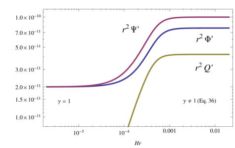
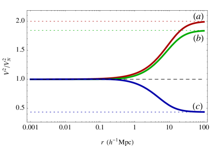
for small , where . A typical behavior of the circular speed divided by the one in general relativity, , is demonstrated in Fig. 5. The line represents the minimally coupled model, corresponds to and . The lines and show the model with and the parameters in and are chosen so that the solutions at short distances become and , respectively. As one can see in Fig. 5, the Vainshtein radius for km/s.
VI Conclusion
Based on the most general scalar-tensor theory with second-order field equations, we have studied metric perturbations on a cosmological background under the influence of the Vainshtein screening mechanism. We have derived the perturbation equations with relevant nonlinearities by taking into account the effects of cosmological background. We have clarified how the Vainshtein mechanism operates in the two subclasses: (i) and (ii) . The situation in the first case is very similar to the Vainshtein mechanism in the Galileon theory, which contains only in the Lagrangian. However, the second case is considered for the first time in a cosmological background in this paper. We have explicitly shown that below the Vainshtein scale there are three possible solutions for : and . We have found that two metric perturbations coincide well inside the Vainshtein radius in the first case, while the parametrized post-Newtonian parameter is related to the propagation speed of gravitational waves, , well inside in the second case. In both cases, Newton’s constant , its time variation , and the parametrized post-Newtonian parameter can be constrained from BBN and the experiments such as lunar laser ranging. These could provide powerful constraints on the most general scalar-tensor theories. In the case , we have demonstrated that the inverse-square law cannot be recovered at sufficiently small .
Acknowledgements.
This work was supported in part by JSPS Grant-in-Aid for Research Activity Start-up No. 22840011 (T.K.), the Grant-in-Aid for Scientific Research No. 21540270 and No. 21244033 and JSPS Core-to-Core Program “International Research Network for Dark Energy”. R.K. acknowledges support by a research assistant program of Hiroshima University.Appendix A Coefficients in the field equations
Here we summarize the definitions of the coefficients in the field equations:
| (75) | |||||
| (76) | |||||
| (77) | |||||
| (78) | |||||
| (79) | |||||
| (80) | |||||
| (81) | |||||
| (82) | |||||
| (83) | |||||
| (84) | |||||
| (85) | |||||
| (86) |
Appendix B Intermediate regime for
Here we would like to point out that there could be an interesting intermediate regime where the quadratic term in Eq. (50) comes into play so that we have the solution
| (87) |
This regime can be found in the range
| (88) |
This intermediate regime can be seen if or ( or ) is sufficiently large (small) compared with others. It is also interesting to see the behavior of the metric perturbations in the intermediate regime (88). In this regime, the metric potentials can be obtained by substituting Eq. (87) into the relations (52),
| (89) | |||
| (90) |
The metric potentials in this regime differ from Eqs. (59) and (67), and the parametrized post-Newtonian parameter ,
| (91) |
is not equal to unity.
We also notice another intermediate regime if is sufficiently large compared with the other coefficients. In this regime becomes constant,
| (92) |
This solution can be seen between Eq. (87) and Eq. (53),
| (93) |
The metric potentials in this regime are given by
| (94) |
Thus, the parametrized post-Newtonian parameter is in this regime. If these regimes (88) and (93) include our solar-system scales, it is possible to constrain the parametrized post-Newtonian parameter as in the former case.
Appendix C Equations in the Fourier space
In this Appendix we summarize the coupled equations for the evolution of the matter density perturbations in Fourier space, which will be useful in the perturbative approach KTH . The matter density perturbations follow
| (95) | |||
| (96) |
where is the velocity field. Assuming the irrotational fluid, we introduce the velocity divergence . Then, due to the Fourier transform, the above equations can be rephrased as
| (97) | |||
| (98) |
Similarly, Eqs. (22), (23), and (25) give
| (99) |
| (100) | |||||
| (101) |
respectively.
References
- (1) A. G. Riess et al., Astron. J. 116, 1009 (1998); Astron. J. 117, 707 (1999); S. Perlmutter et al., Astrophys. J. 517, 565 (1999).
- (2) D. F. Mota and J. D. Barrow, Phys. Lett. B 581, 141 (2004) [arXiv:astro-ph/0306047]; J. Khoury and A. Weltman, Phys. Rev. Lett. 93, 171104 (2004) [arXiv:astro-ph/0309300]; J. Khoury and A. Weltman, Phys. Rev. D 69, 044026 (2004) [arXiv:astro-ph/0309411].
- (3) W. Hu and I. Sawicki, Phys. Rev. D 76, 064004 (2007) [arXiv:0705.1158 [astro-ph]]; A. A. Starobinsky, JETP Lett. 86, 157 (2007) [arXiv:0706.2041 [astro-ph]]; S. A. Appleby and R. A. Battye, Phys. Lett. B 654, 7 (2007) [arXiv:0705.3199 [astro-ph]]; S. Nojiri and S. D. Odintsov, Phys. Rev. D 77, 026007 (2008) [arXiv:0710.1738 [hep-th]].
- (4) A. I. Vainshtein, Phys. Lett. B 39, 393 (1972).
- (5) A. Nicolis, R. Rattazzi, and E. Trincherini, Phys. Rev. D 79, 064036 (2009) [arXiv:0811.2197 [hep-th]].
- (6) K. Koyama, G. Niz, G. Tasinato, Phys. Rev. Lett. 107, 131101 (2011) [arXiv:1103.4708 [hep-th]]; K. Koyama, G. Niz, G. Tasinato, Phys. Rev. D 84, 064033 (2011) [arXiv:1104.2143 [hep-th]];
- (7) G. W. Horndeski, Int. J. Theor. Phys. 10 (1974) 363-384.
- (8) C. Deffayet, G. Esposito-Farese, and A. Vikman, Phys. Rev. D 79, 084003 (2009) [arXiv:0901.1314 [hep-th]]; C. Deffayet, S. Deser, and G. Esposito-Farese, Phys. Rev. D 80, 064015 (2009) [arXiv:0906.1967 [gr-qc]].
- (9) C. Deffayet, X. Gao, D. A. Steer, and G. Zahariade, Phys. Rev. D 84, 064039 (2011) [arXiv:1103.3260 [hep-th]].
- (10) C. Burrage and D. Seery, JCAP 1008, 011 (2010) [arXiv:1005.1927 [astro-ph.CO]]; P. Brax, C. Burrage, and A. -C. Davis, JCAP 1109, 020 (2011) [arXiv:1106.1573 [hep-ph]].
- (11) A. De Felice, R. Kase, and S. Tsujikawa, [arXiv:1111.5090 [gr-qc]].
- (12) K. Koyama and F. P. Silva, Phys. Rev. D 75, 084040 (2007) [hep-th/0702169 [HEP-TH]].
- (13) T. Kobayashi, M. Yamaguchi, and J. Yokoyama, Prog. Theor. Phys. 126, 511-529 (2011). [arXiv:1105.5723 [hep-th]].
- (14) A. De Felice, T. Kobayashi, and S. Tsujikawa, [arXiv:1108.4242 [gr-qc]].
- (15) C. Deffayet, O. Pujolas, I. Sawicki, and A. Vikman, JCAP 1010, 026 (2010). [arXiv:1008.0048 [hep-th]]; O. Pujolas, I. Sawicki, and A. Vikman, arXiv:1103.5360 [hep-th].
- (16) T. Kobayashi, M. Yamaguchi, and J. Yokoyama, Phys. Rev. Lett. 105, 231302 (2010) [arXiv:1008.0603 [hep-th]]; K. Kamada, T. Kobayashi, M. Yamaguchi, and J. Yokoyama, Phys. Rev. D 83, 083515 (2011) [arXiv:1012.4238 [astro-ph.CO]]; T. Kobayashi, M. Yamaguchi, and J. Yokoyama, Phys. Rev. D 83, 103524 (2011) [arXiv:1103.1740 [hep-th]].
- (17) N. Chow and J. Khoury, Phys. Rev. D 80, 024037 (2009) [arXiv:0905.1325 [hep-th]]; F. P. Silva and K. Koyama, Phys. Rev. D 80, 121301 (2009) [arXiv:0909.4538 [astro-ph.CO]]; T. Kobayashi, H. Tashiro and D. Suzuki, Phys. Rev. D 81, 063513 (2010) [arXiv:0912.4641 [astro-ph.CO]]; T. Kobayashi, Phys. Rev. D 81, 103533 (2010) [arXiv:1003.3281 [astro-ph.CO]].
- (18) R. Kimura and K. Yamamoto, JCAP 1104, 025 (2011) [arXiv:1011.2006 [astro-ph.CO]].
- (19) R. Kimura, T. Kobayashi, and K. Yamamoto, arXiv:1110.3598 [astro-ph.CO].
- (20) E. Babichev, C. Deffayet, and G. Esposito-Farese, [arXiv:1107.1569 [gr-qc]].
- (21) J. G. Williams, S. G. Turyshev, and D. H. Boggs, Phys. Rev. Lett. 93, 261101 (2004) [gr-qc/0411113].
- (22) J. -P. Uzan, Living Rev. Rel. 14, 2 (2011) [arXiv:1009.5514 [astro-ph.CO]].
- (23) C. M. Will, Living Rev. Rel. 9, 3 (2005) [gr-qc/0510072].
- (24) D.J. Kapner, T.S. Cook, E.G. Adelberger, J.H. Gundlach, B.R. Heckel, C.D. Hoyle, and H.E. Swanson, Phys. Rev. Lett. 98, 021101 (2007) [hep-th/0611184 [HEP-TH]].
- (25) K. Koyama, A. Taruya, and T. Hiramatsu, Phys. Rev. D 79, 123512 (2009) [arXiv:0902.0618 [astro-ph.CO]]
- (26) T. Narikawa, R. Kimura, T. Yano, and K. Yamamoto [arXiv:1108.2346]