Models for transverse-momentum distributions and transversity

Abstract

I present a short review of models for transverse-momentum distributions and transversity, with a particular attention on general features common to many models. I compare some model results with experimental extractions. I discuss the existence of relations between different functions, their limits of validity, their possible use.

1 Introduction

We believe that the dynamics of quarks and gluons inside the nucleon is described by Quantum ChromoDynamics (QCD). However, due to the difficulty of solving QCD in the nonperturbative regime, we are unable to calculate a priori most of the properties of the nucleon structure, nor to demonstrate directly that QCD leads to parton confinement (see the talk by D. Sivers [1]). The only exception are the studies performed with lattice QCD, which however still present several limitations [2].

In this context, it may be useful to resort to effective models that try to describe the structure of the nucleon using some reasonable simplifications. Models cannot replace full calculations based on the underlying theory. Nevertheless, successful models usually open the way to theoretical advances. A typical example taken from classical mechanics is Kepler’s model of planetary motion, based on elliptical orbits, compared to the standard Copernican model, based on circular motion and epicycles. Kepler’s model was clearly superior in predicting the position of planets. This observation opened the way to the development of Newton’s theory of gravitation.

Nowadays, in the field of hadronic physics, we face the following situation: we have a large (and ever increasing) amount of data, but we cannot compare them with first principle calculations based on QCD. Most of the time, we tend to parametrize the nonperturbative functions involved in physical observables. We are doing something similar to recording the position of planets with high precision. We cannot offer any interpretation of the data. We cannot establish connections between different nonperturbative quantities. We have no reason to trust extrapolations. We are not testing in any way our knowledge of the structure of the proton. At most, we can test the validity of the framework we use to analyze the data, i.e., we can test QCD in the perturbative regime.

In this situation, resorting to models may be essential. It allows us to systematize the information we get from different observables and make predictions based on the assumptions that characterize the model.

There is another crucial issue that makes models almost unavoidable when studying the partonic structure of the nucleon. It is well known that a full information on the “phase-space distribution” of partons can be encoded in Wigner distribution functions [3]. They are Fourier transforms of the so-called Generalized Transverse-Momentum Distributions (GTMDs) [4]. These objects are extremely rich and powerful and give us a picture of the partonic structure of the nucleon in a multidimensional space. Unfortunately, they cannot be probed directly. In specific limits or after specific integrations (see Fig. 1), they reduce to Transverse-Momentum Distributions (TMDs) and Generalized Parton Distributions (GPDs). Further limits/integrations reduce them to collinear Parton Distribution Functions (PDFs) and Form Factors (FFs). These four types of partonic distributions can be extracted from experimental measurements, but often only in limited ranges or limited combinations of the variables involved. In other words, we cannot directly reproduce the full multidimensional picture of the inner structure of the nucleon. At most, we can access some particular projections of the full image.

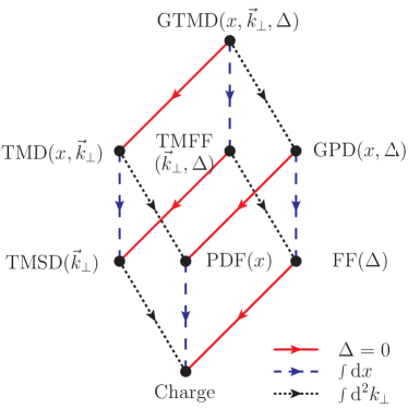
Figure 1: Representation of the projections of the GTMDs into parton distributions and form factors (picture from ref. [5])

We find ourselves as in the Indian story of the blind men and the elephant (I heard this story first from H. Avakian): six blind men were asked to determine what an elephant looked like by feeling different parts of the elephant’s body. Each one feels a different part, but only one part. In the end, each one believes the elephant is something different: a spear (tusk), a fan (ear), a snake (trunk), and so forth. This story illustrates how misleading can be to draw conclusions based on narrow projections of the whole picture.

In this brief review, I give for granted TMD definitions, that can be found, e.g., in refs. [6, 7]

2 Some model results

Many models have been proposed to describe some aspects of the structure of the nucleon. However, not many of them have been used to study TMDs and GPDs. In this talk, I will focus in particular on the following categories of models:

• Light-cone constituent-quark models (LCCQM) [8, 9, 5]

• Spectator models (SM) [10, 11, 12, 13, 14, 15]

• Bag model (BM) [16, 17, 18] and non-relativistic constituent-quark models [19, 20].

• Chiral quark-soliton model ($\chi$QSM) [21, 22, 5]

• Covariant parton model (CPM) [23, 24, 25, 26]

In order to judge the reliability of the models, let us first analyze some well-known functions, i.e., form factors and collinear PDFs. I will present only some selected results, suitable to convey the general message.

In fig. 2, three model calculations of the proton and neutron electric and magnetic form factors are compared to available data.

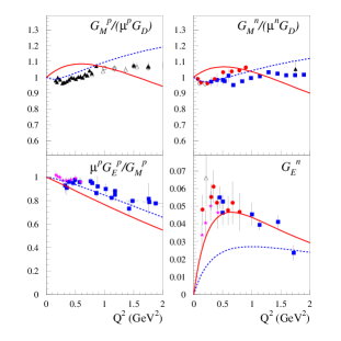
(a)		(b)

Figure 2: The four nucleon electromagnetic Sachs FFs compared to the world data (see [27] and references therein). (a) Calculation in the $\chi$QSM [28] for different values of the constituent quark mass. (b) Solid curves: results in the light-cone $\chi$QSM [5]. Dashed curves: results from the LCCQM [29].

In fig. 3, three model calculations of the up and down unpolarized PDF and helicity PDF are compared to available parametrizations.

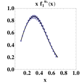
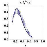
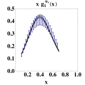
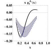
(a)	(b)

Figure 3: The collinear PDFs. (a) Results in the spectator model [14] at 0.3 GeV² compared to the ZEUS02 [30] and GRSV00 [31] parametrizations. (b) Solid curves: results in the $\chi$QSM [5]. Dashed curves: results from the LCCQM [32] at 5 GeV² compared to MSTW09 [33] and LSS07 [34] parametrizations.

I think the general message at this point is the following: models seem to be able to capture the qualitative features of form-factors and collinear PDFs, but they are still far from giving a description that is satisfactory from the quantitative point of view.

Due to the crucial role played at this workshop by the transversity distribution function, I present in fig. 4 several model calculations of the transversity compared to the presently available parametrization of ref. [35].

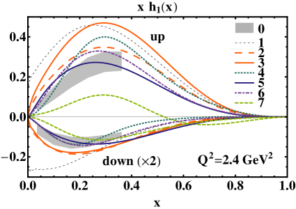
Figure 4: Model calculations of the transversity distribution function compared to available parametrizations: (0–shaded band) extraction from ref. [36]; (1) saturated Soffer bound [37]; (2) $h_{1}=g_{1}$ [38]; (3-4) chiral quark-soliton models [39, 40]; (5) light-cone constituent quark model [41]; (6-7) quark-diquark models [13, 14].

The present extraction of transversity for the up quark is systematically lower than most model calculations, while for the down quark the extraction tends to be bigger than models in absolute value. Two important remarks are in order: first of all, it must be kept in mind that there are no data at $x>0.4$; secondly, it must be stressed that the sign of the up quark distribution cannot be determined from experimental measurements but it is fixed according to the sign of model calculations (interestingly, all of them give the same sign).

Fig. 4 reminds us of another obvious observation: it can often happen that two predictions based on the same type of model give significantly different results. In fig. 4, this occurs for the two $\chi$QSM predictions and the two spectator-model predictions. This is due to different choices in the implementation of the model or simply to different choices for the parameters used in the model.

For what concerns TMDs, we should start from the distribution of unpolarized quarks in an unpolarized nucleon. It has been computed in spectator models [10, 14], LCCQ model [8], $\chi$QS model [22, 5], bag model [18]. However, my impression is that at the moment two important ingredients are missing to allow a fair comparison. From the phenomenology side, the information on the unpolarized TMDs is still limited, in particular in the valence region (see a recent analysis in ref. [42]). From the theory side, model predictions are valid at some low scale, below 1 GeV, that is effectively assumed to be the threshold between the nonperturbative and perturbative regimes. Obviously, comparison with experimental data requires that the predictions are evolved to a higher scale. This demands the application of the correct TMD evolution equations [43, 44], a task that has not been carried out yet. The effect of TMD evolution has been shown to be rather dramatic [44] and tends to broaden the transverse-momentum distribution when the scale increases.

In any case, let me present some numerical results of the models. At a scale of about 0.1 GeV², the LCCQ model of ref. [8, 45] gives a $\langle k_{\perp}^{2}\rangle=0.080$ GeV², and the bag model of ref. [18] gives $\langle k_{\perp}^{2}\rangle=0.077$ GeV² (at $x=0.3$). In these two models, the width is predicted to be the same for up and down quarks (valence only). The spectator model of ref. [14] gives larger widths and different for the two flavors: $\langle k_{\perp u_{v}}^{2}\rangle=0.87$ GeV² and $\langle k_{\perp d_{v}}^{2}\rangle=0.16$ GeV² at a scale of 0.30 GeV². Finally, the $\chi$QSM of ref. [22] predicts $\langle k_{\perp(u+d)}^{2}\rangle=0.18$ GeV² and $\langle k_{\perp(\bar{u}+\bar{d})}^{2}\rangle=0.62$ GeV² at a scale of 0.30-0.40 GeV².

There is a conceptual problem when comparing model TMDs and PDFs to extractions: formally—at least in the present formulation of TMD factorization—collinear PDFs are not the integrals of the corresponding TMDs [43, 44]. The two parton distributions are connected in a more complex way. This may be intuitively understood as follows: the TMD formalism is applicable only when the transverse momentum is much smaller than the dominant hard scale; therefore, after integration it cannot fully reproduce collinear PDFs, which entail an integration over transverse momentum up to a value of the order of the hard scale.

For the moment, let us neglect these problems and turn our attention to another important TMD: the Sivers function [46]. At present, this is the only TMD for which we have a few consistent extractions from experimental data [47, 48, 49, 50, 51, 52, 53]. There is also a long list of model calculations of the Sivers function in the last decade: in spectator models [54, 55, 56, 11, 57, 58, 59, 60, 14], in the bag model [17, 16, 20], in a non-relativistic constituent quark model [19] and a light-cone constituent quark model [9]. In fig. 5 [7], the results of three different calculations of the Sivers function [9, 14, 20] are compared to two of the parametrizations.

Figure 5: Results for the (1)-moments of the quark Sivers function. Solid curves: light-cone constituent quark model of ref. [9]. Dashed curves: spectator model of ref. [14]. Dotted curves: bag model of ref. [17, 20]. Shaded bands correspond to the parametrizations of ref. [50] and [47, 49].

By comparing models with extractions, we can appreciate the fact that models obtain the right sign for the up and down Sivers functions and the right order of magnitude. However, there are large discrepancies in the size. Once again, if we aim at using model for quantitative studies, we need to improve them.

3 Relations among TMDs in models

Model calculations typically have a specific structure and a set of parameters for numerical predictions. If a model disagrees with experimental observations, it may be due to the structure of the model being wrong, or more trivially to the wrong choice of parameters. A powerful way to investigate the structure of the model is to search for relations among predicted quantities, independent of the specific choice of parameters. Several works addressed this question in the last years [61, 62, 63]. Relations based on models have been established among TMDs, between TMDs and PDFs [26], and between TMDs and GPDs [64, 65].

A commonly used set of relations is represented by the so-called Wandzura–Wilczek relations [66]. These relations involve the so-called twist-3 partonic distributions, which typically occur in experimental observables suppressed by a power $M/Q$. At the partonic level, “pure twist-3” usually refers to quark-gluon-quark correlations. The Wandzura–Wilczek approximation consists in removing all pure twist-3 terms. This is strictly speaking possible only for a non-interacting theory, of the kind suggested for instance in the covariant parton model [67] and in ref. [68]. In any theory with interactions the Wandzura–Wilczek relations should break. The group of T-odd TMDs requires final-state interactions and therefore vanishes in Wandzura–Wilczek approximation.

There is no strong evidence yet of the violation of the Wandzura–Wilczek relations. Indications can be found in the structure function $g_{2}$ (see, e.g., ref. [69]) as well as in the fact that the T-odd Sivers function is nonzero [70, 71, 72]. It may nevertheless still be possible to invoke these relations to make semi-quantitative estimates, in particular for T-even TMDs [61].

A second class of relations is represented by the so-called Lorentz-invariance relations. This is actually a misnomer because they are not descending directly from Lorentz invariance. Rather, they originate from neglecting a certain subset of pure twist-3 contributions, namely those related to gauge fields [73, 69]. As for the Wandzura–Wilczek relations, T-odd functions should be zero within these assumptions. Models without gluons respect these relations, while they are obviously spoiled by perturbative QCD, as shown explicitly by the quark-target model [74, 69].

A third class of relations has been observed in a few model calculations (see, e.g., [75] and references therein) and discussed in depth in ref. [63]. They read

$$g_{1}-h_{1}=\tfrac{k_{\perp}^{2}}{2M^{2}}\,h_{1T}^{\perp},$$ (1)

$$g_{1T}=-h_{1L}^{\perp},$$ (2)

$$f_{1T}^{\perp}=h_{1}^{\perp}=0,$$ (3)

$$\left(g_{1T}\right)^{2}+2h_{1}\,h_{1T}^{\perp}=0.$$ (4)

These relations are ascribed to the spherical symmetry of the partonic wave-functions in the canonical-spin basis (together with the possibility of rotating from canonical spin to light-cone spin). They appear to be violated in models with spin-one particles (gluons or axial-vector diquarks). They are violated in perturbative QCD. Nevertheless, they could still be valid approximations at the threshold between the nonperturbative and perturbative regimes. As such, they could be useful conditions to guide TMD parametrizations.

4 Angular momentum and TMDs in models

In general, it is not possible to get direct access to partonic angular momentum using TMDs. This is however possible in the context of models, since they imply characteristic relations between formally independent functions.

A first example has been discussed in a version of the spectator model [76], in the bag model [18] and in the covariant parton model [77] and can be written as

$${\cal L}_{z}^{q}=-\int dxh_{1T}^{\perp(1)q}(x)=\int dx\Bigl{(}h_{1}^{q}(x)-g_{1}^{q}(x)\Bigr{)}.$$ (5)

In the discussion of this relation it has been observed that the identity is valid only at the level of matrix elements, not of operators. If the contributions of all partons are summed, the definition of the orbital angular momentum on the l.h.s. corresponds to that of Jaffe–Manohar. Since the relation has been discussed in a theory without gauge fields, there should be no distinction between the definition of orbital angular momentum according to Jaffe–Manohar and Ji (see, e.g., the discussion in refs. [78, 79]).

A different connection has been explored in ref. [53]. Based on results of spectator models [64, 59, 65, 14, 15] and theoretical considerations [80], the following relation has been used

$$f_{1T}^{\perp(0)q}(x)=-L(x)\,E^{q}(x,0,0),$$ (6)

connecting the Sivers TMD with the GPD $E$ in the forward limit, which is essential to compute angular momentum using Ji’s relation [81]. The above relation can be written in a more general form as a convolution between the “lensing function” $L$ and the GPD $E$. It is actually one of many relations that can be established between TMD and GPDs, which are however also model-dependent [65].

In ref. [53], relation (6) was assumed to be valid and it was shown that it is possible to fit at the same time the nucleon anomalous magnetic moments and data for semi-inclusive single-spin asymmetries produced by the Sivers effect. This analysis leads to the following estimate for quark angular momenta (at $Q^{2}=4$ GeV²)

$$J^{u} =0.229\pm 0.002^{+0.008}_{-0.012}, J^{\bar{u}} =0.015\pm 0.003^{+0.001}_{-0.000},$$ (7)

$$J^{d} =-0.007\pm 0.003^{+0.020}_{-0.005}, J^{\bar{d}} =0.022\pm 0.005^{+0.001}_{-0.000}.$$ (8)

This represents the first model-inspired extraction of partonic angular momentum from TMDs. Strikingly, the results are in agreement with other totally independent estimates [82, 83, 84, 85, 86, 87].

5 Conclusions

A wealth of results concerning transversity and TMDs has been obtained from model calculations in the last decade. Apart from making useful predictions on yet unmeasured quantities, they help us to better understand experimental results. Since they provide relations between different partonic distribution functions, they provide hints on how to reconstruct the full multidimensional structure of the nucleon starting from a limited number of “projections.”

- [1] \NAMESivers D., arXiv:1109.2521.
- [2] \NAMEHagler P., \INPhys. Rept.490201049.
- [3] \NAMEJi X., \INPhys. Rev. Lett.912003062001.
- [4] \NAMEMeissner S., Metz A. \atqueSchlegel M., \INJHEP09082009056.
- [5] \NAMELorce C., Pasquini B. \atqueVanderhaeghen M., \INJHEP11052011041.
- [6] \NAMEBacchetta A., Diehl M., Goeke K., Metz A., Mulders P. J. \atqueSchlegel M., \INJHEP022007093.
- [7] \NAMEBoer D., Diehl M., Milner R., Venugopalan R., Vogelsang W. et al., arXiv:1108.1713.
- [8] \NAMEPasquini B., Cazzaniga S. \atqueBoffi S., \INPhys. Rev. D782008034025.
- [9] \NAMEPasquini B. \atqueYuan F., \INPhys. Rev. D812010114013.
- [10] \NAMEJakob R., Mulders P. J. \atqueRodrigues J., \INNucl. Phys. A6261997937.
- [11] \NAMEBacchetta A., Schäfer A. \atqueYang J.-J., \INPhys. Lett. B5782004109.
- [12] \NAMEGamberg L. P., Goldstein G. R. \atqueSchlegel M., \INPhys. Rev. D772008094016.
- [13] \NAMECloet I. C., Bentz W. \atqueThomas A. W., \INPhys. Lett. B6592008214.
- [14] \NAMEBacchetta A., Conti F. \atqueRadici M., \INPhys. Rev. D782008074010.
- [15] \NAMEBacchetta A., Radici M., Conti F. \atqueGuagnelli M., \INEur. Phys. J. A452010373.
- [16] \NAMEYuan F., \INPhys. Lett. B575200345.
- [17] \NAMECourtoy A., Scopetta S. \atqueVento V., \INPhys. Rev. D792009074001.
- [18] \NAMEAvakian H., Efremov A. V., Schweitzer P. \atqueYuan F., \INPhys. Rev. D812010074035.
- [19] \NAMECourtoy A., Fratini F., Scopetta S. \atqueVento V., \INPhys. Rev. D782008034002.
- [20] \NAMECourtoy A., Scopetta S. \atqueVento V., \INPhys. Rev. D802009074032.
- [21] \NAMEWakamatsu M., \INPhys. Lett. B509200159.
- [22] \NAMEWakamatsu M., \INPhys. Rev. D792009094028.
- [23] \NAMEEfremov A., Teryaev O. \atqueZavada P., \INPhys. Rev. D702004054018.
- [24] \NAMEZavada P., \INEur. Phys. J. C522007121.
- [25] \NAMEEfremov A., Schweitzer P., Teryaev O. \atqueZavada P., \INPhys. Rev. D802009014021.
- [26] \NAMEEfremov A., Schweitzer P., Teryaev O. \atqueZavada P., \INPhys. Rev. D832011054025.
- [27] \NAMEPerdrisat C., Punjabi V. \atqueVanderhaeghen M., \INProg. Part. Nucl. Phys.592007694.
- [28] \NAMEChristov C., Blotz A., Kim H.-C., Pobylitsa P., Watabe T. et al., \INProg. Part. Nucl. Phys.37199691.
- [29] \NAMEPasquini B. \atqueBoffi S., \INPhys. Rev. D762007074011.
- [30] \NAMEChekanov S. et al., \INPhys. Rev. D672003012007.
- [31] \NAMEGlück M., Reya E., Stratmann M. \atqueVogelsang W., \INPhys. Rev. D632001094005.
- [32] \NAMEPasquini B., Pincetti M. \atqueBoffi S., \INPhys. Rev. D762007034020.
- [33] \NAMEMartin A. D., Stirling W. J., Thorne R. S. \atqueWatt G., \INEur. Phys. J. C632009189.
- [34] \NAMELeader E., Sidorov A. V. \atqueStamenov D. B., \INPhys. Rev. D752007074027.
- [35] \NAMEAnselmino M., Boglione M., D’Alesio U., Kotzinian A., Murgia F., Prokudin A. \atqueMelis S., \INNucl. Phys. Proc. Suppl.191200998.
- [36] \NAMEAnselmino M., Boglione M., D’Alesio U., Kotzinian A., Melis S. et al., arXiv:0807.0173.
- [37] \NAMESoffer J., Stratmann M. \atqueVogelsang W., \INPhys. Rev. D652002114024.
- [38] \NAMEKorotkov V. A., Nowak W. D. \atqueOganessyan K. A., \INEur. Phys. J. C182001639.
- [39] \NAMESchweitzer P. et al., \INPhys. Rev. D642001034013.
- [40] \NAMEWakamatsu M., \INPhys. Lett. B6532007398.
- [41] \NAMEPasquini B., Pincetti M. \atqueBoffi S., \INPhys. Rev. D722005094029.
- [42] \NAMESchweitzer P., Teckentrup T. \atqueMetz A., \INPhys. Rev. D812010094019.
- [43] \NAMECollins J. C., Soper D. E. \atqueSterman G., \INNucl. Phys. B2501985199.
- [44] \NAMEAybat S. \atqueRogers T. C., \INPhys. Rev. D832011114042.
- [45] \NAMEBoffi S., Efremov A., Pasquini B. \atqueSchweitzer P., \INPhys. Rev. D792009094012.
- [46] \NAMESivers D. W., \INPhys. Rev. D41199083.
- [47] \NAMEEfremov A. V., Goeke K., Menzel S., Metz A. \atqueSchweitzer P., \INPhys. Lett. B6122005233.
- [48] \NAMEVogelsang W. \atqueYuan F., \INPhys. Rev. D722005054028.
- [49] \NAMECollins J. C. et al., \INPhys. Rev. D732006014021.
- [50] \NAMEAnselmino M. et al., \INEur. Phys. J. A39200989.
- [51] \NAMEArnold S., Efremov A. V., Goeke K., Schlegel M. \atqueSchweitzer P., arXiv:0805.2137.
- [52] \NAMEAnselmino M., Boglione M., D’Alesio U., Melis S., Murgia F. et al., arXiv:1107.4446.
- [53] \NAMEBacchetta A. \atqueRadici M., arXiv:1107.5755.
- [54] \NAMEBrodsky S. J., Hwang D. S. \atqueSchmidt I., \INPhys. Lett. B530200299.
- [55] \NAMEGamberg L. P., Goldstein G. R. \atqueOganessyan K. A., \INPhys. Rev. D672003071504.
- [56] \NAMEGoldstein G. R. \atqueGamberg L., arXiv:hep-ph/0209085.
- [57] \NAMELu Z. \atqueMa B.-Q., \INNucl. Phys. A7412004200.
- [58] \NAMEGoeke K., Meissner S., Metz A. \atqueSchlegel M., \INPhys. Lett. B6372006241.
- [59] \NAMELu Z. \atqueSchmidt I., \INPhys. Rev. D752007073008.
- [60] \NAMEEllis J. R., Hwang D. S. \atqueKotzinian A., \INPhys. Rev. D802009074033.
- [61] \NAMEAvakian H. et al., \INPhys. Rev. D772008014023.
- [62] \NAMEMetz A., Schweitzer P. \atqueTeckentrup T., \INPhys. Lett. B6802009141.
- [63] \NAMELorce C. \atquePasquini B., \INPhys. Rev. D842011034039.
- [64] \NAMEBurkardt M. \atqueHwang D. S., \INPhys. Rev. D692004074032.
- [65] \NAMEMeissner S., Metz A. \atqueGoeke K., \INPhys. Rev. D762007034002.
- [66] \NAMEWandzura S. \atqueWilczek F., \INPhys. Lett. B721977195.
- [67] \NAMEZavada P., \INPhys. Rev. D672003014019.
- [68] \NAMED’Alesio U., Leader E. \atqueMurgia F., \INPhys. Rev. D812010036010.
- [69] \NAMEAccardi A., Bacchetta A., Melnitchouk W. \atqueSchlegel M., \INJHEP09112009093.
- [70] \NAMEAirapetian A. et al., \INPhys. Rev. Lett.942005012002.
- [71] \NAMEAirapetian A. et al., \INPhys. Rev. Lett.1032009152002.
- [72] \NAMEAlekseev M. et al., \INPhys. Lett. B6922010240.
- [73] \NAMEGoeke K., Metz A., Pobylitsa P. V. \atquePolyakov M. V., \INPhys. Lett. B567200327.
- [74] \NAMEKundu R. \atqueMetz A., \INPhys. Rev. D652002014009.
- [75] \NAMEAvakian H., Efremov A., Schweitzer P., Teryaev O., Yuan F. et al., \INMod. Phys. Lett. A2420092995.
- [76] \NAMEShe J., Zhu J. \atqueMa B.-Q., \INPhys. Rev. D792009054008.
- [77] \NAMEEfremov A., Schweitzer P., Teryaev O. \atqueZavada P., \INPoS DIS20102010253.
- [78] \NAMEBurkardt M. \atqueBC H., \INPhys. Rev. D792009071501.
- [79] \NAMEWakamatsu M., \INPhys. Rev. D832011014012.
- [80] \NAMEBurkardt M., \INPhys. Rev. D662002114005.
- [81] \NAMEJi X., \INPhys. Rev. Lett.781997610.
- [82] \NAMEDiehl M., Feldmann T., Jakob R. \atqueKroll P., \INEur. Phys. J. C3920051.
- [83] \NAMEGuidal M., Polyakov M. V., Radyushkin A. V. \atqueVanderhaeghen M., \INPhys. Rev. D722005054013.
- [84] \NAMEAhmad S., Honkanen H., Liuti S. \atqueTaneja S. K., \INPhys. Rev. D752007094003.
- [85] \NAMEGoloskokov S. \atqueKroll P., \INEur. Phys. J. C592009809.
- [86] \NAMEWakamatsu M. \atqueNakakoji Y., \INPhys. Rev. D772008074011.
- [87] \NAMEBratt J. et al., \INPhys. Rev. D822010094502.