Multifractal nature of the surface local density of states in three-dimensional topological insulators with magnetic and nonmagnetic disorder

Abstract

We compute the multifractal spectra associated to local density of states (LDOS) fluctuations due to weak quenched disorder, for a single Dirac fermion in two spatial dimensions. Our results are relevant to the surfaces of $\mathbb{Z}_{2}$ topological insulators such as $\text{Bi}_{2}\text{Se}_{3}$ and $\text{Bi}_{2}\text{Te}_{3}$, where LDOS modulations can be directly probed via scanning tunneling microscopy. We find a qualitative difference in spectra obtained for magnetic versus non-magnetic disorder. Randomly polarized magnetic impurities induce quadratic multifractality at first order in the impurity density; by contrast, no operator exhibits multifractal scaling at this order for a non-magnetic impurity profile. For the time-reversal invariant case, we compute the first non-trivial multifractal correction, which appears at two loops (impurity density squared). We discuss spectral enhancement approaching the Dirac point due to renormalization, and we survey known results for the opposite limit of strong disorder.

I Introduction

The defining attribute of a 3D $\mathbb{Z}_{2}$ topological insulator3DTopIns (TI) is the presence of an odd number of 2D massless Dirac bands at the material surface.KaneHasanREVIEW ; ZhangREVIEW Unlike the Dirac electrons that can appear in a purely 2D system (notably in graphene), the surface states of a (strong) 3D TI are robustly protected from the opening of gap, so long as time-reversal symmetry is preserved. The protection can be viewed as a consequence of the parity anomaly,Semenoff ; RedlichJackiw ; Haldane88 ; ZhangREVIEW which “holographically” links surface states separated by a topologically non-trivial bulk, and gives rise to the signature properties of the $\mathbb{Z}_{2}$ TI state: the half-integer quantum Hall effect, quantized magnetoelectric coupling, “axion” electrodynamics, etc.KaneHasanREVIEW ; ZhangREVIEW As stressed by Schnyder et al. in Ref. SRAL08, , the robust character of the surface states in the presence of quenched disorder can also be taken as a principal characteristic of a topological insulator. In particular, these states are protected from Anderson localization,LeeRamakrishnan even in the presence of a “strong” impurity potential, so long as time-reversal invariance is preserved.Z2Shinsei ; Z2Numerics

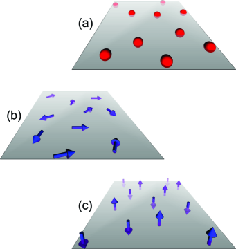
Figure 1: Sketch of disorder “flavors” on the surface of a $\mathbb{Z}_{2}$ topological insulator. In the time-reversal invariant case, the impurities are neutral adatoms or charged dopant ions, depicted as spheres in (a). The effects of these on the surface Dirac theory [Eq. (10)] are encoded in the scalar potential $V(\bm{\mathrm{r}})$. In the case of magnetic disorder, the impurity spins are indicated by the arrows in (b) and (c). In the limit that the spins reside in the plane of the surface, (b), the disorder appears as a vector potential $\bm{\mathrm{A}}(\bm{\mathrm{r}})$. The opposite case of out-of-plane polarization, (c), gives the random mass $M(\bm{\mathrm{r}})$. The case of generic time-reversal breaking disorder has all three potentials present.

With its 2D Dirac band pinned to an exposed surface, a 3D TI is ideally suited to local probes such as scanning tunneling microscopy (STM). In spectroscopic mode, an STM captures an areal map of the local density of states (LDOS). There are several ways of analyzing such data. One is to look for quasiparticle interference (QPI)Capriotti03 ; GuoFranz10 ; QPI-TI-SingImp ; QPI-STM ; Yazdani11 in the LDOS Fourier transform. This method is useful for determining short-distance details, and contains similar information as an analysis of LDOS Friedel oscillations in the presence of a single impurity.SingImpRef It has been applied in TIs to experimental data and analyzed theoretically in Refs. QPI-STM, ; Yazdani11, and GuoFranz10, ; QPI-TI-SingImp, , respectively. In QPI, the disorder is employed primarily as a facilitator to gleam information about the clean system.Capriotti03

Multifractal analysisMFCReview ; Mirlin ; PaladinVulpiani provides a complementary method better suited to extracting large-distance, disorder-dominated features in the same LDOS data field. It is a standard tool for assaying quantum interference phenomena, and is employed in the analysis of wavefunctions near a metal-insulator transitionWegner ; Pruisken ; MFCReview ; Mirlin as well as mesoscopic fluctuations in diffusive metallic systems.Boris ; FalkoEfetov95 In this paper, we derive new results for LDOS multifractal spectra associated to disordered topological insulator surface states. In particular, we extend the pioneering results of Ref. Ludwig94, to the generic cases of time-reversal ($\mathcal{T}$) preserving and breaking impurities. Our calculations are performed in the near-ballistic limit,Schuessler09 wherein weak disorder enters as a perturbation to the clean Dirac band structure. A key characteristic of 2D Dirac fermions is that this weak disorder regime is continuously connected to more conventional domains of multifractal analysis, i.e. the diffusive (symplectic) metalWegner ; FalkoEfetov95 and the integer quantum Hall plateau transition.MFCReview ; PookJanssen91 ; KlesseEvers95 ; ObuseEvers08 These appear at strong coupling (many impurities) for dirty Dirac fermions.Ludwig94 ; Z2Shinsei ; Z2Numerics ; NomuraRyu08

We consider the case of a single flavor Dirac surface band, relevant to (e.g.) the TIs Bi₂Se₃ and Bi₂Te₃ (Refs. KaneHasanREVIEW, ; ZhangREVIEW, ; Bi2X3 BS, ). The different kinds of $\mathcal{T}$-preserving and $\mathcal{T}$-breaking disorder are sketched in Fig. 1. We demonstrate that the LDOS multifractal spectra observed in the absence of time-reversal symmetry breaking (i.e., for non-magnetic disorder) is qualitatively weaker than that induced by magnetic impurities. In particular, the first multifractal correction obtains at first order in the impurity density for the case of broken $\mathcal{T}$, while the first non-trivial amplitude appears at second order in the $\mathcal{T}$-invariant case. We compute the leading terms via one- and two-loop calculations, respectively. We also compute unnormalized spectra for the spin LDOSspinLDOS in the case of magnetic impurities. We show that renormalization effects can enhance multifractality near the Dirac point. Finally, we summarize prior results on various strong-coupling regimes. Our goal is to sketch the full portrait of quantum interference physics on the surface of a TI, valid when interparticle interactions can be neglected.

Our results indicate that the long-distance, disorder-dominated features captured by the multifractal analysis behave in many cases opposite to the short-distance characteristics that appear in quasiparticle interference.GuoFranz10 ; QPI-TI-SingImp ; QPI-STM ; Yazdani11 In Ref. GuoFranz10, , the authors observed that QPI is strongest for the spin LDOS response to magnetic impurities, while the unpolarized LDOS pattern vanishes for magnetic disorder (in the first Born approximation). The QPI response of the LDOS to non-magnetic disorder is weak but non-zero.GuoFranz10 By contrast, in this work we find that the LDOS multifractality is strongest for magnetic impurities, while the spin LDOS spectrum comparatively exhibits the same or weaker strength fluctuations, depending upon the polarization direction.

The weak influence of non-magnetic disorder is tied to the intrinsic spin-orbit coupling that defines the massless Dirac kinetic term. Multifractality is suppressed at one loop due to interference mediated by the Dirac pseudospin, which is proportional to the physical spin on a $\mathbb{Z}_{2}$ insulator surface. The spin is also responsible for the suppression of backscattering from a single non-magnetic impurity.SuppBackScat On the TI surface, magnetic disorder Zeeman couples directly to the Dirac spin, enabling backscattering in near-ballistic transport, and inducing multifractal LDOS fluctuations at the lowest order in the impurity density.

A notable problem in experiments probing topological insulator surface states has been the unintentional doping of carriers into the bulk bands, which then dominate transport measurements in large samples.Transport Even if the chemical potential is moved into the gap, it may reside far from the Dirac point, making it difficult to observe surface state carrier dynamics at low densities. In this respect, STM offers several advantages over transport experiments. First, the position of the chemical potential is no barrier to probing states at the Dirac point, since the latter can always be reached by tuning the bias voltage (although the Dirac point is not guaranteed to reside in the bulk gap).ZhangREVIEW ; Bi2X3 BS Assuming that the Dirac point or the low density regime can be accessed by tuning the tunneling bias, the advent of a finite, even large doping of the surface and/or bulk states may actually play a beneficial role in facilitating the observation of disorder-induced quantum interference effects. This is because a finite carrier density screens the long-range Coulomb potential introduced by charged defects. The potential landscape formed by screened impurities is short-range correlated on scales larger than the screening length. Good screening eliminates the problem of electron and hole puddle formation,Puddles ; PuddlesReview which has until recentlyPuddlesNoMore occluded transport and other properties of Dirac carriers in graphene near the Dirac point. On the other hand, a low density of poorly-screened bulk dopants induces a long-range correlated potential and puddle formation, as in graphene.Yazdani11 LDOS fluctuations in the puddle regime are an important topic for future work.

Three-dimensional topological insulators provide us with an interesting paradigm flip for quantum interference phenomena. Isolating the surface state contribution in transport measurements is problematic. By comparison, direct LDOS imaging is easier than in conventional semiconductor systems, wherein the 2D electron gas is typically buried in a layered material stack. Moreover, the amount of surface disorder can to some extent be controlled; for example, magnetic impurities can be deposited across the surface of an otherwise high-quality bulk 3D sample. These can be charge-neutral adatoms or charged dopants; an example of the former (latter) is provided by iron (manganese)Shen10 in $\text{Bi}_{2}\text{Se}_{3}$.

This paper is organized as follows. We begin in Sec. II with a lightning review of multifractal composite and spin LDOS measures. In Sec. III, we present new results for multifractal LDOS fluctuations in TI surface states, in the presence of weak disorder. We also show how renormalization can enhance multifractality close to the Dirac point. Finally, in Sec. IV, we review previous results on various strong disorder regimes relevant to the $\mathbb{Z}_{2}$ TI surface states and LDOS statistics. In particular, we discuss the symplectic metal, the integer quantum Hall plateau transition, and the Anderson insulator. Various technical details are relegated to appendices. In Appendix A, we review the symmetry classes of Anderson (de)localization that appear in the disordered Dirac surface theory. In Appendix B, we supply some details of our perturbative calculations.

II Multifractal LDOS measures

II.1 Definitions

We suppose that the tunneling local density of states (LDOS) $\nu(\varepsilon,\bm{\mathrm{r}})$ is imaged at a fixed energy $\varepsilon$ over an $L\times L$ field of view. The field is finely partitioned into a grid of boxes. The box edge length $a\ll L$ must be chosen larger than any “microscopic” scale $l_{\mathsf{m}}$, such as the correlation length of the random potential.MFCReview One introduces the box probability

$$\mu_{n}(\varepsilon)\equiv\frac{\int\limits_{\mathcal{A}_{n}}d^{2}\bm{\mathrm{r}}\,\nu(\varepsilon,\bm{\mathrm{r}})}{\sum_{l}\left[\int\limits_{\mathcal{A}_{l}}d^{2}\bm{\mathrm{r}}\,\nu(\varepsilon,\bm{\mathrm{r}})\right]},$$ (1)

where $\mathcal{A}_{n}$ denotes the $n^{\text{th}}$ box. LDOS multifractality is defined through the inverse of the participation ratio (IPR),Wegner ; MFCReview

$$\mathcal{P}_{q}(\varepsilon)\equiv\sum_{n}\mu_{n}^{q}(\varepsilon)\sim\left(\frac{a}{L}\right)^{\tau(q,\varepsilon)}.$$ (2)

The right-hand side (scaling limit) obtains when $l_{\mathsf{m}}\ll a\ll L$; corrections are down by higher powers of $a/L$. The exponent $\tau(q,\varepsilon)$ is the multifractal moment spectrumHalsey ; MFCReview for LDOS fluctuations at energy $\varepsilon$.

The construction in Eqs. (1) and (2) is useful for characterizing a system with extended states, or for an Anderson localized system in which $L\ll\xi_{\mathsf{loc}}(\varepsilon)$; $\xi_{\mathsf{loc}}$ denotes the localization length. In what follows, we assume experiments are performed at sufficiently low temperatures so that inelastic cutoffs to quantum interference can be ignored.LeeRamakrishnan ; WRM A clean system with plane wave states at energy $\varepsilon$ has $\tau(q,\varepsilon)=2(q-1)$. Multifractality refers to the incorporation of corrections non-linear in $q$. Physically, these arise due to quantum interference via multiple scattering of electron waves in a dirty environment, processes that serve as the precursor to Anderson localization.Wegner ; MFCReview ; Boris

For weak disorder, the spectrum is typically dominated by the quadratic correctionWegner ; MFCReview

$$\tau(q,\varepsilon)=2(q-1)-\theta(\varepsilon)\,q(q-1),$$ (3)

where $\theta\geq 0$ gives a measure of the disorder strength. As an example, in a weakly disordered 2D metal (with $L\ll\xi_{\mathsf{loc}}$ for the orthogonal or unitary classes), one findsWegner ; Pruisken ; FalkoEfetov95

$$\theta=\frac{\beta^{-1}}{2\pi^{2}N(\varepsilon)D},$$ (4)

where $N(\varepsilon)$ denotes the average density of states, $D$ is the classical (Drude) diffusion constant, and $\beta\in\{1,2,4\}$, depending upon the presence or absence of time-reversal symmetry and spin-orbit scattering.FalkoEfetov95 ; RandomMatrix At stronger disorder, higher order corrections in $\theta q$ must be retained; for the diffusive metals, results are known to four loops.Wegner

An alternative characterization of LDOS multifractality is provided by the singularity spectrumHalsey ; MFCReview $f(\alpha)$: Over a subset of the sample grid area that scales as $(L/a)^{f(\alpha)}$, the box probability $\mu\sim(a/L)^{\alpha}$. The singularity spectrum is the Legendre transform of $\tau(q)$,

$$f(\alpha)=q\alpha-\tau(q),\quad\frac{d\tau(q)}{dq}=\alpha.$$

For the quadratic spectrum in Eq. (3), one obtains

$$f(\alpha)=2-\frac{1}{4\theta}\left(\alpha-2-\theta\right)^{2}.$$ (5)

In this “parabolic approximation,” the strength of the multifractality is encoded in the peak position $\alpha_{0}$ [$f(\alpha_{0})=2$], and the width $\alpha_{\mathsf{W}}$ of the spectrum such that $f(\alpha_{0}\pm\alpha_{\mathsf{W}}/2)=0$,

$$\alpha_{0}=2+\theta,\quad\alpha_{\mathsf{W}}=4\sqrt{2\theta}.$$ (6)

Part of the power of multifractal analysis for disordered quantum systems derives from the fact that the spectra [$\tau(q)$ or $f(\alpha)$] typically depend only upon a few gross measures of the impurity potential. In the case of dirty metals, the entire spectrum can be computed as an expansion in one parameter, the inverse conductance (consistent with scaling theory).Wegner ; LeeRamakrishnan ; Boris At a non-interacting Anderson localization transition, $\tau(q)$ and $f(\alpha)$ become universal functions, so that the critical point is characterized by an infinite set of critical exponents [e.g., the expansion coefficients for $\tau(q)$].

The spectra above have been defined for data collected in a single fixed realization of the disorder. Strictly speaking, Eq. (3) then applies only for $|q|\leq q_{c}$, where $q_{c}=\sqrt{2/\theta}$. Outside of this range, the $\tau(q)$ associated to a fixed disorder realization is linear, a phenomenon known as spectral termination.Chamon96 ; Castillo97 ; Foster09 [This assumes that higher order corrections can be ignored for $q\geq q_{c}$. Regardless, the $\tau(q)$ spectrum is always linear for sufficiently large $q$]. Termination can be viewed as a consequence of the restriction to positive sample measures $f(\alpha)\geq 0$.Halsey ; Mirlin

In the localized regime, the states contributing to the LDOS at a given position in the sample have a discrete energy spectrum, quantized by the typical localization volume $\xi_{\mathsf{loc}}^{2}$. As a result, all non-unity LDOS moments diverge in the absence of level smearing. In a tunneling experiment, smearing can appear due to inelastic scattering (temperature), open sample boundary conditions, or due to the finite energy resolution of the instrument. To characterize an Anderson insulating state over an $L\times L$ field of view with $L\gg\xi_{\mathsf{loc}}$, the full LDOS distribution should be examined;AltPrig87 ; Lerner88 sensitive dependence of the distribution shape to smearing can serve as a telltale sign of the localized regime. LDOS fluctuations in the Anderson insulator are reviewed in more detail in Sec. IV.2.

II.2 Spin LDOS spectra

By restricting the character of the tunneling species, it may be possible to measure individual LDOS components separately. For example, in the case of a spin-polarized (ferromagnetic) STM tip,spinLDOS the spin-projected components $\nu_{\uparrow,\downarrow}$ can be separately resolved. The use of an unpolarized tip recovers the composite LDOS $\nu=\nu_{\uparrow}+\nu_{\downarrow}$. We define the spin LDOS along the spin space direction $\hat{\iota}$,

$$\nu^{\hat{\iota}}(\varepsilon,\bm{\mathrm{r}})\equiv\nu^{\hat{\iota}}_{\uparrow}(\varepsilon,\bm{\mathrm{r}})-\nu^{\hat{\iota}}_{\downarrow}(\varepsilon,\bm{\mathrm{r}}).$$ (7)

For a time-reversal invariant system (with or without spin-orbit scattering and/or disorder), one has $\nu^{\hat{\iota}}(\varepsilon,\bm{\mathrm{r}})=0$. In a system with broken time-reversal (e.g., magnetic impurities), but zero average spin polarization, the integral of $\nu^{\hat{\iota}}(\varepsilon,\bm{\mathrm{r}})$ over a sufficiently large region becomes arbitrarily small; we cannot use the normalized construction in Eqs. (1) and (2) to characterize spin LDOS multifractals. Instead, we employ the un-normalized inverse spin participation ratio (ISPR)

$$\mathcal{P}^{\hat{\iota}}_{q}(\varepsilon)\equiv\sum_{n}\left(\mu_{n}^{\hat{\iota}}\right)^{q},\quad\mu_{n}^{\hat{\iota}}\equiv\int\limits_{\mathcal{A}_{n}}d^{2}\bm{\mathrm{r}}\,\nu^{\hat{\iota}}(\varepsilon,\bm{\mathrm{r}}).$$ (8)

In the scaling limit,

$$\mathcal{P}^{\hat{\iota}}_{q}(\varepsilon)\sim c_{q}\left(\frac{a}{L}\right)^{x_{q}^{\hat{\iota}}-2},$$ (9)

where the exponent $x_{q}^{\hat{\iota}}$ is the scaling dimension for the corresponding moment operator in the disorder-averaged field theory description, and $c_{q}\neq 0$ for even $q$.

III Weak disorder multifractality

III.1 Model. Short- and long-range correlated potential landscapes

The Dirac surface states of a $\mathbb{Z}_{2}$ topological insulator (TI) are guaranteed to appear in an odd number of flavors.KaneHasanREVIEW ; ZhangREVIEW In this paper, we consider the simplest case of a single flavor, relevant to (e.g.) $\text{Bi}_{2}\text{Se}_{3}$ and $\text{Bi}_{2}\text{Te}_{3}$. The Hamiltonian is (in units such that $\hbar=1$)

$$H=\!\int\!d^{2}\bm{\mathrm{r}}\,\psi^{\dagger}\!\left\{\begin{aligned} &v_{F}\,\hat{\sigma}_{\mu}\left[-i\partial_{\mu}+A_{\mu}(\bm{\mathrm{r}})\right]\\ &\,+M(\bm{\mathrm{r}})\,\hat{\sigma}_{3}+V(\bm{\mathrm{r}})\end{aligned}\right\}\!\psi,$$ (10)

where $\mu\in\{1,2\}$, and repeated indices are summed. The coordinates $\bm{\mathrm{r}}=\{x,y\}$ chart the TI surface, while the topological bulk resides in the perpendicular $z$ direction. In Eq. (10), $v_{F}$ denotes the Fermi velocity, and the Dirac pseudospin Pauli matrices $\hat{\bm{\sigma}}$ are related to the physical spin $1/2$ operators $\hat{\bm{S}}$ via $\{\hat{\sigma}_{\mu},\hat{\sigma}_{3}\}=2\{\epsilon_{\mu\nu}S_{\nu},S_{3}\}$. The vector, scalar, and mass potentials $\{\bm{\mathrm{A}},V,M\}$ describe the effects of external electromagnetic fields and/or surface impurities. In the absence of time-reversal ($\mathcal{T}$) symmetry breaking, $\bm{\mathrm{A}}=M=0$. (See Appendix A for an enumeration of discrete symmetry operations.) Thus, a mass gap is explicitly forbidden so long as $\mathcal{T}$ remains a good symmetry, a consequence of the protection afforded by the topologically nontrivial bulk. When $\mathcal{T}$ is broken by an external magnetic field $\bm{\mathrm{B}}$, the vector and mass potentials are

$$A_{\mu} =-eA_{\mu}^{(\mathsf{orb})}-\frac{\gamma_{{\scriptstyle{\parallel}}}}{2v_{F}}\epsilon_{\mu\nu}B_{{\scriptstyle{\parallel}},\nu},$$

$$M =-\frac{\gamma_{\perp}}{2}B_{z},$$ (11)

where $\gamma_{{\scriptstyle{\parallel}}}$ ($\gamma_{\perp}$) denotes the Zeeman coupling to the in-plane field $\bm{\mathrm{B}}_{{\scriptstyle{\parallel}}}$ (out-of-plane field $B_{z}$), and the orbital effect is embedded in $A_{\alpha}^{(\mathsf{orb})}$ via $\epsilon_{\alpha\beta}\partial_{\alpha}A_{\beta}^{(\mathsf{orb})}=B_{z}$.

Non-magnetic adatoms or charge traps are encoded in the scalar potential $V(\bm{\mathrm{r}})$. In-plane (out-of-plane) polarized magnetic impurities additionally induce point exchange coupling to the vector $\bm{\mathrm{A}}(\bm{\mathrm{r}})$ [mass $M(\bm{\mathrm{r}})$] fields.SingImpRef The different types of disorder leading to $V$, $\bm{\mathrm{A}}$, and $M$ are sketched in Fig. 1. Assuming a random surface distribution of impurities and spatial rotational invariance on average, the disorder potentials can be taken as Gaussian white noise distributed variables,

$$\begin{aligned} \overline{V(\bm{\mathrm{r}})V(\bm{\mathrm{r^{\prime}}})}&=\Delta_{V}\,v_{F}^{2}\,\delta(\bm{\mathrm{r}}-\bm{\mathrm{r^{\prime}}}),\\ \overline{A_{\alpha}(\bm{\mathrm{r}})A_{\beta}(\bm{\mathrm{r^{\prime}}})}&=\Delta_{A}\,v_{F}^{2}\,\delta_{\alpha\beta}\,\delta(\bm{\mathrm{r}}-\bm{\mathrm{r^{\prime}}}),\\ \overline{M(\bm{\mathrm{r}})M(\bm{\mathrm{r^{\prime}}})}&=\Delta_{M}\,v_{F}^{2}\,\delta(\bm{\mathrm{r}}-\bm{\mathrm{r^{\prime}}}).\end{aligned}$$ (12)

The dimensionless variances $\Delta_{V,A,M}$ quantify the disorder strength. In the first Born approximation, these are of the form

$$\Delta\,v_{F}^{2}=n_{\mathsf{imp}}|\tilde{u}(0)|^{2},$$ (13)

where $n_{\mathsf{imp}}$ is the impurity density, and $\tilde{u}(\bm{\mathrm{q}})$ denotes the Fourier transform of the single impurity potential. We note that a net in-plane magnetization of the surface impurities $\overline{A^{\mu}}\neq 0$ can be removed by a gauge transformation, while the average scalar potential $\overline{V}$ is absorbed into the chemical potential. We will assume that there is no net magnetization perpendicular to the surface, $\overline{M}=0$, or that we only probe LDOS fluctuations on energy scales much larger than the induced gap $2v_{F}\overline{M}$.

In 2D, the single impurity potential $u(\bm{\mathrm{r}})$ [Eq. (13)] must decay faster than $1/r^{2}$ (or oscillate rapidly enough) so that the limit $\tilde{u}(\bm{\mathrm{q}}\rightarrow 0)$ exists; otherwise, the white noise assumption in Eq. (12) is invalidated by long range impurity potential correlations.LRCorrDirt This causes a problem for charged impurities, which can become poorly screened for a small surface doping relative to the Dirac point. In graphene, the long-range correlated potential undulations induced by poorly-screened substrate impurities leads to a smearing of the Dirac point over an energy scale $k_{B}T_{\mathsf{rms}}\propto v_{F}\sqrt{n_{\mathsf{imp}}}$, and to the breakup of the sample into electron and hole puddles.Puddles ; PuddlesReview The advent of electron-hole puddles has until recently prevented the observation of various “intrinsic” phenomena associated to the Dirac carriers in graphene experiments such as velocity renormalizationPuddlesNoMore and hydrodynamic transport near the Dirac point. In this respect, a large surface or bulk doping actually improves the situation for STM measurement of disorder-induced quantum interference, since these carriers screen the potential of surface charges. The disorder potential can be considered short-range correlated for scales larger than the screening length.

If we consider only surface doping, with an insulating bulk, then the Thomas-Fermi wavelength due to a finite surface carrier density $n$ is given by

$$\lambda_{\mathsf{TF}}=\frac{1}{\alpha}\sqrt{\frac{\pi}{n}},$$ (14)

where $\alpha\equiv e^{2}/\epsilon v_{F}$ is the effective “fine structure constant.” The permittivity $\epsilon=(1+\epsilon_{\text{TI}})/2$, the average of the bulk TI below and vacuum above the surface. For $\text{Bi}_{2}\text{Se}_{3}$ with a surface density of $n=7\times 10^{12}$ $\text{cm}^{-2}$ (corresponding to a doping level of $0.3$ eV relative to the Dirac point),Bi2X3 BS $v_{F}=5\times 10^{5}$ m/s (Ref. Bi2X3 BS, ), and permittivityBi2Se3Diel $\epsilon_{\text{TI}}=113$, one obtains $\lambda_{\mathsf{TF}}\sim 90$ nm. This is very large, and indicates that the surface state carrier density is inadequate to screen charged impurities. A smaller screening length is possible for bulk doping,Yazdani11 or by performing experiments on thin film samples exfoliated over a metallic gate. Alternatively, one can restrict the deposition of surface impurities to non-doping adatoms, e.g. iron in $\text{Bi}_{2}\text{Se}_{3}$.Shen10 The disorder variance associated to Thomas-Fermi screened charged impurities is

$$\Delta_{V}=\pi\frac{n_{\mathsf{imp}}}{n}.$$ (15)

Finally, we note that the appearance in isolation of any of the three disorder potentials in Eq. (10) realizes three different symmetry classes of Anderson (de)localization,Classes ; BernardLeClair ; SRAL08 see Appendix A for a review. The $\mathcal{T}$-invariant case with $\Delta_{A,M}=0$ belongs to the spin-orbit class AII, which is also the class of the $\mathbb{Z}_{2}$ topological bulk [Fig. 1(a)]. In the case of broken $\mathcal{T}$, $\Delta_{V,M}=0$ realizes the random vector potential model in class AIII [Fig. 1(b)], while $\Delta_{V,A}=0$ gives the random mass model in class D [Fig. 1(c)]. All three classes exhibit delocalized states in 2D, although this occurs only at the Dirac point for class AIII.Ludwig94 In the $\mathcal{T}$-invariant symplectic case, the unpaired single Dirac flavor avoids the usual spin-orbit metal-insulator transition,Z2Numerics remaining delocalized even for strong disorder due to a topological term.Z2Shinsei The generic case of broken-$\mathcal{T}$ with all three disorder potentials non-zero realizes the unitary class A, and is believed to flow under renormalization to the plateau transition in the integer quantum Hall effect.Ludwig94 ; NomuraRyu08 (See Sec. IV.1.2 for a review).

Because in-plane (out-of-plane) Zeeman coupling appears in the vector (mass) potential [Eq. (III.1)], one is tempted to identify class AIII (class D) with the limit of an otherwise clean surface, dusted with charge neutral magnetic impurities randomly polarized in-plane (perpendicular to the TI surface). However, a magnetic adatom is expected to also induce a local scalar potential deformation $V(\bm{\mathrm{r}})$. For example, it can dope the surface or bulk, as occurs for a manganese impurity in $\text{Bi}_{2}\text{Se}_{3}$ (Ref. Shen10, )]. As discussed in Appendix A, the advent of any two flavors of disorder destroys the additional discrete symmetries enjoyed by the special class D and AIII Hamiltonians. The asymptotic long-distance LDOS scaling is then governed by the unitary class A, discussed above. Nevertheless, depending upon the relative microscopic strength of the magnetic versus potential perturbations induced by polarized magnetic impurities, the class AIII or D model may provide an adequate approximation for broken-$\mathcal{T}$ LDOS fluctuations on intermediate scales.

III.2 Results

To compute the scaling of LDOS moments in a quantum theory with quenched disorder, one employs a path integral $Z$ to express products of fermion Green’s functions as functionals of the disorder configuration. Using a trick (replicas,Wegner ; LeeRamakrishnan ; Boris supersymmetry,SUSY or KeldyshKeldysh ) to normalize $Z=1$, the Green’s functions are formally averaged over disorder configurations (typically with a Gaussian weight). The result is a translationally-invariant, but “interacting” field theory, where the disorder strength $\Delta$ appears as a coupling constant.LeeRamakrishnan ; SUSY Perturbative calculations are controlled via loop expansion for small $\Delta$.

To determine the scaling, one decomposes the $q^{\text{th}}$ LDOS moment into projections upon the renormalization group (RG) eigenoperators of the disorder-averaged theory.Wegner ; Pruisken ; Boris The multifractal spectrum $\tau(q)$ is determined by the most relevant (negative)Duplantier scaling dimension $x_{q}$ exhibited by an eigenoperator in this decomposition, and is given byMirlin ; Foster09

$$\tau(q)=2(q-1)+x_{q}-qx_{1}.$$ (16)

III.2.1 Broken $\mathcal{T}$: random vector potential disorder (Class AIII)

The properties of the model in Eq. (10) with short-range correlated disorder [Eq. (12)] were originally studied in Ref. Ludwig94, . In this work, the exact multifractal spectrum $\tau(q)$ was calculated for the broken-$\mathcal{T}$, random vector potential ($\sim$ in-plane polarized magnetic impurity)Footnote–IsolatedDisorder class AIII model, to all orders in $\Delta_{A}$. Technically, this result obtains because the disorder-averaged AIII model is conformally invariant at the Dirac point, and the exact LDOS moment spectra can be extracted using an Abelian bosonization treatment. The exact spectrumLudwig94 is quadratic in $q$, and takes the form of Eq. (3), with

$$\theta_{A}=\frac{\Delta_{A}}{\pi}.$$ (17)

Subsequent workChamon96 ; Castillo97 on the random vector potential model elucidated the mechanisms of termination and freezing, transitions that occur in the spectral statistics for large moments $q>q_{c}(\Delta_{A})$ or strong disorder $\Delta_{A}\geq 2\pi$.

For this broken-$\mathcal{T}$ class, we can also examine the spin LDOS fluctuations, utilizing the same nonperturbative bosonization treatment employed in Ref. Ludwig94, . The spin LDOS $\nu^{\hat{\iota}}(\varepsilon,\bm{\mathrm{r}})$ taken along an axis $\hat{\iota}$ in spin space was defined by Eq. (7). Moment fluctuations are characterized by the inverse spin participation ratio (ISPR) in Eq. (8), the scaling limit of which is controlled by the dimension $x_{q}^{\hat{\iota}}$ that appears in Eq. (9). The out-of-plane ISPR $\mathcal{P}^{\hat{3}}_{q}(\varepsilon)$ is associated to the “mass” fermion bilinear $\nu^{\hat{3}}=\psi^{\dagger}\hat{\sigma}_{3}\psi$. For the random vector potential model, the most relevant contribution to $\mathcal{P}^{\hat{3}}_{q}(\varepsilon)$ carries the same scaling dimension that gives the composite LDOS scaling in Eqs. (3) and (17),

$$x_{q}^{\hat{3}}=q-\frac{\Delta_{A}}{\pi}q^{2}.$$ (18)

The chiral components of the in-plane spin LDOS are the energy-resolved $U(1)$ Dirac current operators

$$\nu^{\pm}\equiv\nu^{\hat{1}}\pm i\nu^{\hat{2}}=\psi^{\dagger}\hat{\sigma}_{\pm}\psi.$$ (19)

Moments of these are RG eigenoperators that receive no corrections. The scaling of the associated ISPR is governed by the disorder-independent (tree level) exponent

$$x_{q}^{\pm}=q.$$ (20)

Eqs. (17), (18), and (20) are exact results that hold to all orders in $\Delta_{A}$.

III.2.2 Broken $\mathcal{T}$: random mass disorder (Class D)

In the rest of this section, we provide new results for the broken-$\mathcal{T}$, random mass ($\sim$ out-of-plane polarized magnetic impurity)Footnote–IsolatedDisorder class D model, the $\mathcal{T}$-invariant class AII model, and the generic broken-$\mathcal{T}$ unitary class A model. For weak disorder, none of these are conformally invariant, and we resort to perturbation theory. In this section we summarize results; some technical aspects are sketched in Appendix B. The results obtained below hold only for small $\Delta_{V,M}\ll 1$, wherein the disorder appears as a weak marginal perturbation (at tree level) to the clean Dirac surface band structure.

For the broken-$\mathcal{T}$ case of random mass disorder (with $\Delta_{V}=\Delta_{A}=0$), one obtains quadratic multifractality at one loop, again governed by Eq. (3), with

$$\theta_{M}=\frac{\Delta_{M}}{2\pi}+\bm{\mathit{O}}\left(\Delta_{M}^{2}\right).$$ (21)

Moments of the out-of-plane spin LDOS operator $\nu^{\hat{3}}=\psi^{\dagger}\hat{\sigma}_{3}\psi$, as well as of the chiral in-plane [$U(1)$ current] operators $\nu^{\pm}=\psi^{\dagger}\hat{\sigma}_{\pm}\psi$ constitute RG eigenoperators at one loop, with scaling dimensions

$$x_{q}^{\hat{3}}= q+\frac{\Delta_{M}}{2\pi}q+\bm{\mathit{O}}\left(\Delta_{M}^{2}\right),$$ (22)

$$x_{q}^{\pm}= q+\bm{\mathit{O}}\left(\Delta_{M}^{2}\right).$$ (23)

Note that the first correction in Eq. (22) is positive (and linear in $q$); this should be contrasted with the AIII case, Eq. (18) above. On general grounds, the anomalous scaling dimension associated to the $q^{\text{th}}\geq 1$ moment of the composite LDOS, or any projected component thereof, must appear with a negative sign. The reason is that this quantity is associated to a moment of a normalized probability distributionMFCReview ; Duplantier through Eqs. (1) and (2). For a quadratic $\tau(q)$ spectrum, this leads in particular to $\theta\geq 0$ in Eq. (3) [consistent with a positive, real disorder variance—c.f. Eqs. (17), (21), and (24)]. By contrast, the spin LDOS is defined as the difference between two orthogonal projections [Eq. (7)]; for this reason, the first disorder correction to the scaling dimension in Eq. (22) is not required to appear with a particular sign.

III.2.3 Non-magnetic disorder (Class AII)

In the $\mathcal{T}$-invariant case of scalar potential disorder, it turns out that no local operator (without derivatives) exhibits multifractal scaling to first order in $\Delta_{V}$. For Dirac fermions, this applies to both LDOS and energy-resolved current moments. Physically, the weak influence of non-magnetic disorder is due to interference mediated by the Dirac pseudospin (equivalent to physical spin $1/2$ on the TI surface). The Dirac pseudospin is also responsible for the suppression of backscattering from a single non-magnetic impurity.SuppBackScat Technically, this result is derived by mapping the one-loop renormalization process of local operators to the action of a certain spin-$1/2$ Hamiltonian $H^{(\mathsf{eff})}_{V}$, and identifying renormalization group eigenoperators with states that diagonalize $H^{(\mathsf{eff})}_{V}$ (see Appendix B). As a result, to lowest order one observes plane wave scaling in the LDOS IPR [Eq. (2)]. The spin LDOS vanishes exactly, due to $\mathcal{T}$.

The first non-trivial correction to the LDOS $\tau(q)$ appears at two loops. To this order, the spectrum is again quadratic as in Eq. (3). A straight-forward but laborious calculation gives the coefficient in this equation,

$$\theta_{V}=\frac{3\Delta_{V}^{2}}{8\pi^{2}}+\bm{\mathit{O}}\left(\Delta_{V}^{3}\right).$$ (24)

Since $\Delta_{V}\propto n_{\mathsf{imp}}$ [Eqs. (13) or (15)], we find that the non-trivial multifractal scaling begins at second order in the impurity density. This is qualitatively weaker than any of the broken-$\mathcal{T}$ regimes, where the quadratic multifractality appears already at first order, Eqs. (17) and (21). This distinction between $\mathcal{T}$-invariant and $\mathcal{T}$-broken surfaces is our primary result, and can be tested directly in STM experiments by varying the concentration of deposited surface disorder. Although the $\mathcal{T}$-invariant case is not conformally invariant (for a discussion of renormalization effects, see Sec. III.3, below), the multifractal $\tau(q)$ and $f(\alpha)$ spectra depend only upon a single parameter, the variance $\Delta_{V}$. Eq. (24) can be extended to higher loops, allowing ever more precise tests against numerics or experimental data within the perturbatively accessible regime. The multifractal spectrum therefore provides a unique fingerprint for the time-reversal invariant Dirac surface state of the $\mathbb{Z}_{2}$ topological insulator, in the presence of weak but otherwise generic non-magnetic disorder. The opposite limit of strong disorder for the $\mathcal{T}$-invariant case is discussed below in Sec. IV.1.1.

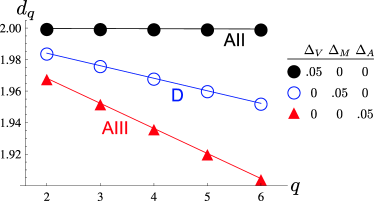
Figure 2: Quadratic multifractality for isolated disorder flavors. The Renyi dimension $d_{q}=2-\theta\,q$ [Eqs. (3) and (25)] is plotted for the exact vector potential (AIII), one-loop mass (D), and two-loop scalar potential (symplectic AII) results [Eqs. (17), (21), and (24)]. The disorder strength is $\Delta=0.05$ for each case. The broken time-reversal class D and AIII corrections appear at order $\Delta_{M,A}$, while the (much weaker) time-reversal invariant class AII correction begins at order $\Delta_{V}^{2}$.

III.2.4 Broken $\mathcal{T}$: generic disorder (Class A)

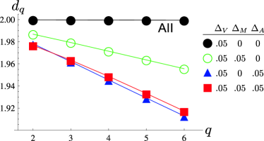
Figure 3: One-loop Renyi dimensions [Eq. (25)] in the broken $\mathcal{T}$, multidisorder unitary class A case, for various disorder strength combinations. These results were obtained by numerically extracting the largest positive eigenvalue from the effective spin Hamiltonian $H^{\mathsf{eff}}$ in Eq. (53) (restricting the search to operators invariant under spatial rotations and reflections); see Appendix B for details. The two-loop result for the $\mathcal{T}$-invariant case is shown for reference.

When $\mathcal{T}$ is broken and any two disorder flavors appear, the system resides in the unitary class A. The third disorder flavor is always generated under renormalization—see Sec. III.3, below. The results of Eqs. (17) and (21) for the LDOS $\tau(q)$ spectrum in the random vector and mass potential models suggest that the unitary case also exhibits multifractality to first order in the impurity density $n_{\mathsf{imp}}$, since $\Delta_{A,M,V}\propto n_{\mathsf{imp}}$.

With multiple flavors of the disorder, solving the operator mixing problem for the $q^{\text{th}}$ LDOS moment requires the diagonalization of an effective spin Hamiltonian $H^{(\mathsf{eff})}$, transcribed in Eq. (53) of Appendix B. In Figs. 3 and 4, we present the results obtained by numerically diagonalizing this matrix for various combinations of $\{\Delta_{V},\Delta_{M},\Delta_{A}\}$. In these figures we plot the Renyi dimensionPaladinVulpiani $d_{q}$, defined for $q\neq 1$ via

$$d_{q}\equiv\frac{\tau(q)}{q-1}.$$ (25)

Figs. 3 and 4 show that the generic broken-$\mathcal{T}$ case is multifractal at one loop, and easily distinguished from the two-loop $\mathcal{T}$-invariant result, in the limit of weak disorder. [Note that Fig. 4 indicates that the $\tau(q)$ spectrum is not purely quadratic in this general case.] It should therefore be possible to precisely distinguish the broken-$\mathcal{T}$ and $\mathcal{T}$-invariant spectra experimentally, by observing the dependence of the deviation $2-d_{q}$ on $n_{\mathsf{imp}}$. The single-disorder flavor results for comparable strengths are plotted in Fig. 2 for reference.

For the multidisorder unitary model, the same RG eigenoperators dominate the scaling of composite $\nu$ and out-of-plane spin $\nu^{\hat{3}}$ LDOS moments. The dimension $x_{q}^{\hat{3}}$ that determines the spin LDOS scaling via Eq. (9) also enters into the LDOS spectrum in Eq. (16), leading to Figs. 3 and 4. By contrast, moments of the chiral spin LDOS components $\nu^{\pm}$ [Eq. (19)] remain eigenoperators that acquire no corrections at one loop,

$$x_{q}^{\pm}=q+\bm{\mathit{O}}\left(\Delta_{\alpha}\Delta_{\beta}\right),$$ (26)

$\alpha,\beta\in\{A,M,V\}$.

As reviewed in the subsequent Sec. IV.1.2, for $\overline{M}=0$, the generic broken-$\mathcal{T}$ model is believed to flow to the critical state at the integer quantum Hall plateau transition.Ludwig94 ; NomuraRyu08 This state exhibits strong multifractality that has been extensively studied in numerics.MFCReview ; Mirlin ; PookJanssen91 ; KlesseEvers95 ; ObuseEvers08

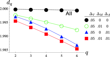
Figure 4: The same as Fig. 3, but for different unitary class disorder strength combinations. In the data presented here, $\Delta_{V}>\Delta_{M,A}$. Regardless, the one-loop spectrum obtained for either $\Delta_{M,A}>0$ is stronger than the two loop $\mathcal{T}$-invariant case with $\Delta_{M}=\Delta_{A}=0$. The latter is also shown for reference.

III.3 Renormalization effects

As discussed at the beginning of the previous section, the disorder-averaged Dirac surface state theory used to compute LDOS multifractal spectra is an “interacting” field theory, wherein the disorder strengths $\Delta_{V,A,M}$ appear as coupling constants (c.f. Appendix B). Because these parameters are dimensionless, at weak coupling the disorder constitutes a marginal perturbation of the clean Dirac band structure. The one-loop RG equations for these parameters are given byLudwig94 ; Mirlin1loopRG

$$\frac{d\Delta_{A}}{dl} =\frac{1}{\pi}\Delta_{M}\Delta_{V},$$ (27a)

$$\frac{d\Delta_{M}}{dl} =\frac{1}{\pi}\left(2\Delta_{A}-\Delta_{M}\right)\left(\Delta_{M}+\Delta_{V}\right),$$ (27b)

$$\frac{d\Delta_{V}}{dl} =\frac{1}{\pi}\left(2\Delta_{A}+\Delta_{V}\right)\left(\Delta_{M}+\Delta_{V}\right),$$ (27c)

where $l=\log L$ denotes the log of the RG length scale (e.g., the system size). Energy $\varepsilon$ scales as

$$\frac{d\ln\varepsilon}{dl}=z(l),$$ (28)

where the (scale-dependent) dynamic critical exponent is

$$z=1+\frac{1}{2\pi}\left(2\Delta_{A}+\Delta_{M}+\Delta_{V}\right)+\bm{\mathit{O}}\left(\Delta_{\alpha}\Delta_{\beta}\right),$$ (29)

$\alpha,\beta\in\{A,M,V\}$.

In this section, we use Eqs. (27)–(29) to derive the dynamical scaling of the disorder parameters $\Delta_{V,A,M}(\varepsilon)$; here energy $\varepsilon$ is measured relative to the Dirac point, not the Fermi energy. (From the point-of-view of the disordered Dirac theory, a finite energy above the Dirac point constitutes a relevant perturbation.Ludwig94 ) Using the results obtained in the previous section, we thereby determine the enhancement or suppression of LDOS multifractality approaching the Dirac point, due to renormalization.

III.3.1 Broken $\mathcal{T}$: random vector potential disorder (Class AIII)

For the random vector potential model with $\Delta_{V}=\Delta_{M}=0$, Eq. (27) implies

$$\frac{d\Delta_{A}}{dl}=0,$$

so that $\Delta_{A}=\Delta_{A}^{{\scriptscriptstyle{(}}\circ{\scriptscriptstyle{)}}}$ (constant), where $\Delta_{A}^{{\scriptscriptstyle{(}}\circ{\scriptscriptstyle{)}}}$ is the “microscopic” value derived from the randomly polarized in-plane magnetic impurity distribution.Footnote–IsolatedDisorder This result in fact holds to all orders in $\Delta_{A}$;Ludwig94 in this case, the theory describing LDOS fluctuations at the Dirac point is conformally invariant. Multifractality is neither enhanced nor suppressed as one moves away from the Dirac point, defined as $\varepsilon=0$. However, for non-zero energies $\varepsilon\neq 0$, in an infinite size sample all states are in fact localized.Ludwig94 The localization length diverges upon approaching the band center as $\xi_{\mathsf{loc}}(\varepsilon)\sim\varepsilon^{-1/z}$, with $z=1+\Delta_{A}/\pi$ [Eq. (29)]. Eqs. (3) and (17) for $\tau(q)$ hold on scales smaller than $\xi_{\mathsf{loc}}(\varepsilon)$.

III.3.2 Broken $\mathcal{T}$: random mass disorder (Class D)

For the random mass model with $\Delta_{V}=\Delta_{A}=0$,

$$\frac{d\Delta_{M}}{dl}=-\frac{\Delta_{M}^{2}}{\pi}+\bm{\mathit{O}}\left(\Delta_{M}^{3}\right),$$

so that the disorder is marginally irrelevant at weak coupling.Ludwig94 Integrating this equation and using Eqs. (28) and (29), we can compute the scaling of $\Delta_{M}$ with energy. At energy scale $\Upsilon$, we define $\Delta_{M}^{{\scriptscriptstyle{(}}\circ{\scriptscriptstyle{)}}}\equiv\Delta_{M}(\Upsilon)$; then for the smaller energy scale $\varepsilon$ (relative to the Dirac point), we obtain the logarithmic suppression

$$\Delta_{M}(\varepsilon\lesssim\Upsilon)\sim \,\Delta_{M}^{{\scriptscriptstyle{(}}\circ{\scriptscriptstyle{)}}}-\frac{\left(\Delta_{M}^{{\scriptscriptstyle{(}}\circ{\scriptscriptstyle{)}}}\right)^{2}}{\pi}\log\left(\frac{\Upsilon}{\varepsilon}\right)$$

$$+{\bm{\mathit{O}}}\left\{\left[\Delta_{M}^{{\scriptscriptstyle{(}}\circ{\scriptscriptstyle{)}}}\left(1-\frac{\varepsilon}{\Upsilon}\right)\right]^{2}\!,\left(\Delta_{M}^{{\scriptscriptstyle{(}}\circ{\scriptscriptstyle{)}}}\right)^{3}\right\}\!.$$ (30)

This equation holds for $|1-\varepsilon/\Upsilon|\ll 1$. In the limit as $\varepsilon\rightarrow 0$, the disorder strength vanishes as

$$\Delta_{M}(\varepsilon\rightarrow 0)\sim \pi\left[\ln\left(\sqrt{\frac{\pi}{\Delta_{M}^{{\scriptscriptstyle{(}}\circ{\scriptscriptstyle{)}}}}}\frac{\Upsilon}{\varepsilon}\right)\right]^{-1}$$

$$+\bm{\mathit{O}}\left[\frac{1}{\Delta_{M}^{{\scriptscriptstyle{(}}\circ{\scriptscriptstyle{)}}}}\ln^{-2}\left(\sqrt{\frac{\pi}{\Delta_{M}^{{\scriptscriptstyle{(}}\circ{\scriptscriptstyle{)}}}}}\frac{\Upsilon}{\varepsilon}\right)\right].$$ (31)

For small $\Delta_{M}^{{\scriptscriptstyle{(}}\circ{\scriptscriptstyle{)}}}$, Eq. (III.3.2) applies only at very small energies $\varepsilon\lesssim\Upsilon\exp(-1/\Delta_{M}^{{\scriptscriptstyle{(}}\circ{\scriptscriptstyle{)}}})$.

III.3.3 Non-magnetic disorder (Class AII)

Now we consider the $\mathcal{T}$-invariant model. The flow equation for $\Delta_{V}$ is

$$\frac{d\Delta_{V}}{dl}=\frac{\Delta_{V}^{2}}{\pi}+\bm{\mathit{O}}\left(\Delta_{V}^{3}\right).$$ (32)

In contrast to the random mass, the random scalar potential is a marginally relevant perturbation to the clean band structure.Ludwig94 Examining lower and lower energy scales approaching the Dirac point, one observes stronger effects of the disorder. In the asymptotic scaling limit wherein the impurity potential strength becomes “large” ($\Delta_{V}\gtrsim 1$), numericalZ2Numerics results and analyticalZ2Shinsei arguments imply that the disordered $\mathcal{T}$-invariant Dirac theory renormalizes into the “conventional” symplectic metal. The metal is distinguished from the Dirac theory by its non-zero (and non-critical) density of states at zero energy,LeeRamakrishnan and by its $\tau(q)$ spectrum.Wegner ; FalkoEfetov95 We discuss the strong coupling LDOS multifractality below in Sec. IV.1.1. If at energy $\Upsilon$, $\Delta_{V}(\Upsilon)\equiv\Delta_{V}^{{\scriptscriptstyle{(}}\circ{\scriptscriptstyle{)}}}\ll 1$, then for a somewhat smaller energy $\varepsilon$ we obtain the logarithmic enhancement

$$\Delta_{V}(\varepsilon\lesssim\Upsilon)\sim \Delta_{V}^{{\scriptscriptstyle{(}}\circ{\scriptscriptstyle{)}}}+\frac{\left(\Delta_{V}^{{\scriptscriptstyle{(}}\circ{\scriptscriptstyle{)}}}\right)^{2}}{\pi}\log\left(\frac{\Upsilon}{\varepsilon}\right)$$

$$+{\bm{\mathit{O}}}\left\{\left[\Delta_{V}^{{\scriptscriptstyle{(}}\circ{\scriptscriptstyle{)}}}\left(1-\frac{\varepsilon}{\Upsilon}\right)\right]^{2}\!,\left(\Delta_{V}^{{\scriptscriptstyle{(}}\circ{\scriptscriptstyle{)}}}\right)^{3}\right\}\!.$$ (33)

Eq. (III.3.3) implies that renormalization strengthens multifractality approaching the Dirac point $\varepsilon=0$, for the $\mathcal{T}$-invariant case. We emphasize that this has nothing to do with weak (anti-)localization. The latter occurs in the diffusive metallic regime with $k_{F}l_{\mathsf{mfp}}\gg 1$, where $l_{\mathsf{mfp}}$ denotes the elastic mean free path. The diffusive regime obtains at strong couplingZ2Numerics near the Dirac point $k_{F}\rightarrow 0$ [Sec. IV.1.1, below]. The impurity strength renormalization in Eq. (III.3.3) is a quantum effect deriving from the clean band structure, in the “near-ballistic” regime.Schuessler09

III.3.4 Broken $\mathcal{T}$: generic disorder (Class A)

In the generic case of broken $\mathcal{T}$, with multiple disorder coupling strengths non-zero, the system flows toward strong coupling $\Delta_{V,M,A}\rightarrow\infty$. As a result, multifractality is enhanced approaching the Dirac point. The RG flow ultimately terminates at a strong coupling critical point, or in the Anderson insulator, discussed in the next section.

IV Strong coupling regimes

In this section, we review prior results on strong coupling regimes relevant to the disordered Dirac $\mathbb{Z}_{2}$ topological insulator surface states, LDOS fluctuations and associated multifractal spectra. These are not new, but provide complimentary information to the new results derived in the previous section.

In both generic cases of $\mathcal{T}$-invariant, and $\mathcal{T}$-breaking impurities, the disordered Dirac description used in Sec. III fails on the largest length and lowest energy scales (approaching charge neutrality). For a sufficiently dilute concentration impurities, the results obtained in the previous section characterize the start of the scaling regime, over energy and length scales such that the disorder strengths remain weak $\Delta_{V,A,M}(L,\varepsilon)\ll 1$. When these parameters become order one (due to renormalization down to lower energies and longer lengths), the system crosses over to one of the strong coupling regimes discussed below.

IV.1 Delocalized states at strong disorder

IV.1.1 $\mathcal{T}$-invariant case: diffusive metal via strong disorder

In a random scalar potential field, the Dirac point vacillates in energy with spatial location; as a result, the density of states near charge neutrality is enhanced by the disorder. Due to the suppression of pure backscattering for Dirac fermions,SuppBackScat the state density enhancement more than compensates for the increased scattering introduced by the additional impurities. As a result, scalar potential disorder actually increases the (zero temperature, Landauer) conductance at charge neutrality beyond the clean ballistic result, $e^{2}/\pi h$ (Refs. Z2Numerics, ; Schuessler09, ). As in Sec. III, here we assume short-range correlated disorder, due either to charge neutral impurities or efficient screening by bulk and/or surface carriers. We do not discuss the puddle regimePuddles ; PuddlesReview in the present paper.

The effective disorder strength $\Delta_{V}$ is enhanced by renormalization, as indicated by the runaway flow implied by Eq. (32). The concomitant density of states and conductance growth suggests that the disordered Dirac theory ultimately crosses over to the ordinary diffusive symplectic metal, a result born out by numerics.Z2Numerics In the absence of time-reversal symmetry breaking, Anderson localization is prohibited on the surface of a topological insulator.SRAL08 ; Z2Shinsei

The symplectic metal possesses a finite (non-critical) average density of states at charge neutrality, and a distinct $\tau(q)$ spectrum. For a large effective diffusion constant $D$ (induced for a Dirac fermion subject to sufficiently strong disorder,Z2Numerics or for a weakly disordered system examined on large length scales), the lowest order result for the multifractal spectrum appears in Eqs. (3) and Eq. (4), above. In the latter equation, $\beta=4$ for the symplectic class.FalkoEfetov95 ; RandomMatrix

For the $\mathcal{T}$-invariant case, the strongest multifractality is expected at intermediate coupling. Weak disorder $\Delta_{V}\ll 1$ induces weak multifractality in the Dirac language [$\tau(q)$ in Eqs. (3) and (24)], while strong disorder ultimately pushes the system into the symplectic metal, where a large diffusion constant $D$ suppresses the first correction in Eq. (4).

IV.1.2 Broken $\mathcal{T}$: IQHP transition

For generic $\mathcal{T}$-breaking disorder, i.e. all three $\Delta_{V,M,A}$ non-zero, the disordered Dirac theory is also unstable under renormalization. When the average mass is zero $\overline{M}=0$ (see below), the flow in Eq. (27) is believed to terminate at the critical point of the integer quantum Hall plateau transition.Ludwig94 ; NomuraRyu08 This is the delocalized state separating adjacent Hall plateaux; it exhibits strong multifractality that has been extensively studied in numerics.MFCReview ; PookJanssen91 ; KlesseEvers95 ; ObuseEvers08 The spectrum is believed to be universal,MFCReview and is approximatelyObuseEvers08 parabolic as in Eqs. (3) and (5), with $\theta\sim 0.26$ (Refs. KlesseEvers95, ; ObuseEvers08, ).

IV.2 Anderson insulator

At zero chemical potential relative to the Dirac point, an average out-of-plane spin magnetization at the surface of a $\mathbb{Z}_{2}$ TI corresponds to the presence of a non-zero Dirac mass $M$ for the surface carriers. This insulating state resides in a quantum Hall plateau [with $\sigma_{xy}=\operatorname{sgn}(M)\,e^{2}/2h$].Haldane88 ; Ludwig94 ; KaneHasanREVIEW ; ZhangREVIEW In the presence of surface disorder, the plateau state will assume the character of a localized Anderson insulator. In this section we review LDOS fluctuations in the Anderson insulator. The discussion is relevant not only to the magnetized surface of a 3D TI, but also to localized states populating the bulk gap of a disordered TI. Proposals exploiting localization to realize so-called “topological Anderson insulators” by adding impurities to clean hosts include those in Ref. TopAndIns, .

To understand local density of states fluctuations in an Anderson insulator, it is useful to first study a toy problem. Consider a tight-binding model on a $d-$dimensional lattice, subject to nearest-neighbor hopping $t$, and a random on-site potential $V_{i}$, distributed uniformly over the region $-W/2\leq V_{i}\leq W/2$. We assume the absence of spatial correlations in the disorder potential. The inverse relative strength of the disorder is measured by the ratio $t/W$. We consider first the extreme limit of zero hopping, $t/W\rightarrow 0$. In that case, the LDOS is the on-site operator

$$\nu_{i}(\varepsilon,V_{i})=\frac{\eta/\pi}{\left(\varepsilon-V_{i}\right)^{2}+\eta^{2}},$$

where $\eta$ denotes an energy-smearing parameter. Physically, smearing is determined by inelastic scattering, open sample boundary conditions, or due to the finite energy resolution of the probing instrument.

At the “band center” $\varepsilon=0$, the distribution function for disorder-averaged LDOS moments evaluates to

$$p(\nu)\equiv \int_{-W/2}^{W/2}\frac{dV}{W}\delta\left[\nu-\nu\left(\varepsilon,V\right)\right]$$

$$= \frac{1}{\pi\nu^{2}W}\sqrt{\frac{\nu}{\nu_{\mathsf{max}}-\nu}}.$$ (34)

In this equation, the LDOS is constrained to the interval $\nu_{\mathsf{min}}\leq\nu\leq\nu_{\mathsf{max}}$, where

$$\nu_{\mathsf{min}}=\frac{4\eta}{\pi\left(W^{2}+4\eta^{2}\right)},\quad\nu_{\mathsf{max}}=\frac{1}{\pi\eta}.$$ (35)

Using Eq. (IV.2), one can compute the disorder-averaged moments of the LDOS,

$$\overline{\nu^{q}}=\frac{\Gamma\left(q-\frac{1}{2}\right)}{W\pi^{q-1/2}\Gamma(q)}\eta^{1-q}.$$ (36)

The average LDOS is $\overline{\nu}=1/W$; all higher moments are proportional to $\eta^{1-q}$, and thus diverge in the limit of zero energy smearing $\eta\rightarrow 0$. This not surprising, because the energy spectrum in our trivial toy model is discrete, so that the LDOS operator becomes a delta function with ill-defined moments as $\eta\rightarrow 0$. The moments are dominated by the power-law (Pareto) tail of the distribution, accumulating at the upper limit $\nu=\nu_{\mathsf{max}}$. By contrast, the typical LDOS, defined as ${\nu}_{\mathsf{typ}}=\exp(\overline{\log\nu})$ is dominated by the infrared

$${\nu}_{\mathsf{typ}}=\frac{4\eta e^{2}}{\pi W^{2}}.$$

This vanishes in the limit $\eta\rightarrow 0$.

We see that observables exhibit broad statistics in the single site model, governed by the $p(\nu)\sim\nu^{-3/2}$ power-law distribution in Eq. (IV.2). The moments are rendered finite only by the non-zero energy smearing parameter $\eta$. This should be compared to the LDOS statistics in a system with extended states and weak multifractality, e.g. that characterized by the quadratic $\tau(q)$ spectrum in Eq. (3), with $0<\theta\ll 1$. It is knownBoris that the corresponding LDOS distribution has a Gaussian bulk, with a small amplitude log-normal tail responsible for the weak multifractality. For the metallic system, the result is independent of energy smearing, provided that the thermodynamic limit is taken before the smearing is set to zero. Returning to the toy insulator model, we observe that the global density $\nu_{G}$ of states (GDOS) is self-averaging in the same limit. The GDOS is defined via

$$\nu_{G}\equiv\frac{1}{N}\sum_{i=1}^{N}\nu_{i}(V_{i}),$$

where $N$ denotes the number of sites. In the large $N$-limit, the cumulant expansion can be evaluated via the saddle-point. The cumulants of the GDOS then take the form

$$\overline{\left[\nu_{G}\right]^{q}_{c}}=N^{1-q}\,\left(\overline{\nu^{q}}+\ldots\right),$$

where $\left[\cdots\right]^{q}_{c}$ denotes the $q^{\text{th}}$ cumulant, and the omitted terms are smaller by positive powers of $\eta$. Taking the infinite system size limit $N\rightarrow\infty$ before sending the energy smearing to zero $\eta\rightarrow 0$ leads to the vanishing of all $q>1$ GDOS cumulants.

The calculations above can be extended to non-zero hopping via a locator expansion in small $t/W$, as performed by Anderson in his original 1958 paper.Anderson58 This expansion can be formally summed to all orders in 1D and on the Bethe lattice,BetheLat but an explicit solution for the LDOS statistics is difficult to obtain this way; see Ref. SUSY, for an alternative approach.

Altshuler and PrigodinAltPrig87 succeeded in deriving the distribution generating disorder-averaged LDOS moments in a 1D system, which is exponentially localized for arbitrarily weak disorder.LeeRamakrishnan In the thermodynamic limit for a closed sample, they obtain the “inverse Gaussian” distribution

$$p(\tilde{\nu})=\sqrt{\frac{4\eta}{\pi\epsilon}}\frac{1}{\tilde{\nu}^{3/2}}\exp\left[-\frac{4\eta}{\epsilon}\frac{(\tilde{\nu}-1)^{2}}{\tilde{\nu}}\right],$$ (37)

where $\tilde{\nu}\equiv\nu/\overline{\nu}$, and $\epsilon$ is the typical energy level spacing in a localization volume; $\epsilon^{-1}$ is also the elastic scattering lifetime.AltPrig87 In the limit of small smearing $\eta\ll\epsilon$, this distribution has moments

$$\overline{\tilde{\nu}^{q}} =\frac{4^{1-q}\Gamma\left(q-\frac{1}{2}\right)}{\sqrt{\pi}}\left(\frac{\eta}{\epsilon}\right)^{1-q}.$$ (38)

The exact result in Eq. (38) for the 1D Anderson insulator exhibits the same singular dependence on the energy smearing $\eta$ as the single site model moment in Eq. (36). In fact, the distributions in Eqs. (IV.2) and (37) are very similar: both feature a $\nu^{-3/2}$ power law at intermediate $\nu$, while the exponential factor in Eq. (37) plays the role of the hard cutoffs $\nu_{\mathsf{min},\mathsf{max}}$ in Eqs. (IV.2) and (35). The close resemblance of the exact 1D and single site model results can be attributed to the discrete spectrum of energy levels contributing to the LDOS in an Anderson insulator, with an energy level spacing determined by the localization volume $\xi_{\mathsf{loc}}^{d}$ in $d$ spatial dimensions.

The take away is that the LDOS distribution in an Anderson insulator becomes very broad, with a power-law tail yielding divergent moments, in the limit of vanishingly small energy smearing. In an STM experiment performed at ultra-low temperature, on a large, isolated Anderson localized surface, the collected LDOS statistics should be very sensitive to the smearing induced by the energy resolution of the measurement itself.

The locally discrete energy spectrum of the LDOS in the Anderson insulator invalidates the use of Eq. (2) as a tool to compute the multifractal $\tau(q)$ spectrum. As advocated above, the shape of the LDOS distribution function and its sensitivity to smearing can best reveal the insulating phase. If one insists upon computing moments, one must employWegner

$$\tau^{(\mathsf{loc})}(q) \equiv-\frac{d}{d\ln L}\,\overline{\ln\left[\frac{1}{\overline{\nu}}\int_{L^{d}}d^{d}\bm{\mathrm{r}}\,\sum_{i}|\psi_{i}(\bm{\mathrm{r}})|^{2q}\delta\left(\varepsilon-\varepsilon_{i}\right)\right]}.$$ (39)

Since the levels are discrete,

$$\lim_{\eta\rightarrow 0}(\pi\eta)^{q-1}\nu^{q}(\varepsilon,\bm{\mathrm{r}})=\sum_{i}|\psi_{i}(\bm{\mathrm{r}})|^{2q}\delta\left(\varepsilon-\varepsilon_{i}\right).$$ (40)

Thus,

$$\tau^{(\mathsf{loc})}(q)= -\frac{d}{d\ln L}\,\ln\left\{\int_{L^{d}}d^{d}\bm{\mathrm{r}}\,\left[\lim_{\eta\rightarrow 0}(\pi\eta)^{q-1}\overline{\nu^{q}(\varepsilon,\bm{\mathrm{r}})}\right]\right\}$$

$$+\frac{d}{d\ln L}\,\ln\left\{\int_{L^{d}}d^{d}\bm{\mathrm{r}}\,\overline{\nu(\varepsilon,\bm{\mathrm{r}})}\right\}.$$ (41)

In this equation, we replace averages-of-the-logs with logs-of-the-average, a procedure that is legitimate here because spatial and disorder-averaging are expected to yield the same results on the insulating side. Noting that the LDOS moments are $L$-independent in the insulator for $L\gg\xi_{\mathsf{loc}}$, we obtain the expected resultMFCReview for localized states

$$\tau^{(\mathsf{loc})}(q)=0,$$ (42)

computed in a well-defined $\eta\rightarrow 0$ limit.

V Acknowledgments

The author thanks Kostya Kechedzhi for a collaboration that lead to this work, and thanks Andreas Ludwig, Igor Aleiner, Pedram Roushan, Haim Beidenkopf, Emil Yuzbashyan, and Deepak Iyer for useful discussions. The author acknowledges support by the National Science Foundation under Grant No. DMR-0547769, and by the David and Lucile Packard Foundation.

Appendix A Discrete symmetries, random matrix classification, and disorder

The 10 symmetry classes of disordered Hamiltonians (Hermitian random matrices) can be efficiently distinguished by the presence or absence of time-reversal $\mathcal{T}$, particle-hole $\mathcal{P}$, and chiral/“sublattice” symmetry $\mathcal{C}$.Classes ; BernardLeClair ; SRAL08 For the two-component Dirac Hamiltonian in Eq. (10), the definitions of these symmetries are essentially unique. In terms of the two-component Dirac spinor $\psi$, these appear as

$$\mathcal{T}: \psi \rightarrow-i\hat{\sigma}_{2}\psi,\quad i\rightarrow-i$$ (43a)

$$\mathcal{P}: \psi \rightarrow\hat{\sigma}_{1}\left[\psi^{\dagger}\right]^{\mathsf{T}},$$ (43b)

$$\mathcal{C}: \psi \rightarrow\hat{\sigma}_{3}\left[\psi^{\dagger}\right]^{\mathsf{T}},\quad i\rightarrow-i.$$ (43c)

In the second quantized language, $\mathcal{T}$ and $\mathcal{C}$ are antiunitary transformations; the unitary $\mathcal{P}$ can be taken as the product of these.

The imposition of any one of the discrete symmetries upon the Hamiltonian in Eq. (10) in every disorder realization restricts its form, and selects a particular random matrix symmetry class.Ludwig94 ; Classes ; BernardLeClair ; SRAL08 (1) $\mathcal{T}$-invariance: $\bm{\mathrm{A}}=M=0$, only potential disorder $\Delta_{V}\geq 0$ is allowed. Since $\mathcal{T}^{2}=-1$, this is the symplectic (spin-orbit) class AII, which is also the symmetry class of the (presumed $\mathcal{T}$-invariant) topological $\mathbb{Z}_{2}$ bulk. (2) $\mathcal{P}$-invariance: $V=\bm{\mathrm{A}}=0$, only random mass disorder $\Delta_{M}\geq 0$ is allowed. Because $\mathcal{P}^{2}=+1$, this is the broken time-reversal class D. (3) $\mathcal{C}$-invariance: $V=M=0$, only random vector potential disorder $\Delta_{A}\geq 0$ is allowed. This is the broken time-reversal class AIII. (Technically, it is the “topological”/WZW class $\text{AIII}_{1}$ in the language of Refs. SRAL08, ; BernardLeClair, .)

Class AII is generically realized whenever time-reversal is unbroken. Magnetic impurities randomly polarized parallel (perpendicular) to the TI surface manifest as point exchange sources in the vector (mass) potentials of Eq. (10); we are thus tempted to identify symmetry classes D and AIII with these two limits. However, a magnetic impurity will typically induce a local potential fluctuation $V(\bm{\mathrm{r}})$ as well. As a consequence, the generic case of broken-time reversal symmetry corresponds to the absence of $\mathcal{T},\mathcal{P}$, and $\mathcal{C}$, which gives the unitary class A.Classes ; BernardLeClair ; SRAL08 In fact, for a vanishing average mass $\overline{M}=0$, the surface of a topological insulator with generic time-reversal breaking disorder is expected to flow under renormalization to the critical point of the integer quantum Hall plateau transition.Ludwig94 ; NomuraRyu08 On a different note, the class $\text{AIII}_{1}$ and class D versions of $H$ in Eq. (10) can be realized on the surface of a bulk $\mathcal{T}$-invariant 3D topological superconductor, where time-reversal is respectively preserved or broken at the surface.SRAL08

Appendix B Perturbation theory

B.1 Chiral Decomposition and one-loop renormalization

We write a 2+0-D fermion path integral to represent correlation functions in the disordered Dirac Hamiltonian transcribed in Eq. (10). The fermion operators are replaced with the Grassmann fields $\{\psi,\psi^{\dagger}\}\rightarrow\{\psi_{i},\bar{\psi}_{i}\}$; here $i\in\{1,\ldots,n\}$ denotes a replica index, and we are to send $n\rightarrow 0$ at the end of the calculation.Wegner ; LeeRamakrishnan We employ a “chiral decomposition” of the two-component spinors,

$$\psi_{i}=\begin{bmatrix}L_{i}\\ R_{i}\end{bmatrix},\quad\bar{\psi}_{i}=\begin{bmatrix}\bar{R}_{i}&\bar{L}_{i}\end{bmatrix}$$ (44)

Then the action of the replicated theory is

$$\mathcal{S}=\int\!d^{2}\bm{\mathrm{r}}\!\left[\begin{aligned} &\varepsilon\left(\bar{R}_{i}L_{i}+\bar{L}_{i}R_{i}\right)+\bar{R}_{i}L_{i}\phi+\bar{L}_{i}R_{i}\bar{\phi}\\ &+\bar{R}_{i}\left(-i\partial+A\right)R_{i}+\bar{L}_{i}\left(-i\bar{\partial}+\bar{A}\right)L_{i}\end{aligned}\right],$$ (45)

where we have introduced complex coordinates $\{z,\bar{z}\}=x\pm iy$, $\{\partial,\bar{\partial}\}=(\partial_{x}\mp i\partial_{y})$, and disorder potentials $\{A,\bar{A}\}=A_{x}\mp iA_{y}$, $\{\phi,\bar{\phi}\}=V\pm M$. The energy $\varepsilon$ is a fixed parameter. In Eq. (45), repeated replica indices are summed. Assuming the Gaussian white-noise variances for the disorder potentials enumerated in Eq. (12), the replicated theory can be averaged over disorder configurations. The post-ensemble averaged action is

$$\overline{\mathcal{S}}=\mathcal{S}_{0}+\overline{\mathcal{S}}_{A}+\overline{\mathcal{S}}_{1}+\overline{\mathcal{S}}_{2},$$ (46)

where $\mathcal{S}_{0}$ is the clean Dirac action, and

$$\overline{\mathcal{S}}_{A}= -2\Delta_{A}\int d^{2}\bm{\mathrm{r}}\,\bar{R}_{i}R_{i}\bar{L}_{j}L_{j},$$ (47a)

$$\overline{\mathcal{S}}_{1}= -\frac{\Delta_{V}+\Delta_{M}}{2}\int d^{2}\bm{\mathrm{r}}\,\left(\bar{R}_{i}L_{i}\bar{R}_{j}L_{j}+\bar{L}_{i}R_{i}\bar{L}_{j}R_{j}\right),$$ (47b)

$$\overline{\mathcal{S}}_{2}= -(\Delta_{V}-\Delta_{M})\int d^{2}\bm{\mathrm{r}}\,\bar{R}_{i}L_{i}\bar{L}_{j}R_{j}.$$ (47c)

Different replicas become coupled through the disorder.Wegner ; LeeRamakrishnan

The disorder-averaged composite LDOS $\overline{\nu}(\varepsilon,\bm{\mathrm{r}})$ corresponds to the fermion bilinear expectation

$$\overline{\nu}=\langle\bar{\psi}\psi\rangle=\langle\bar{R}L+\bar{L}R\rangle.$$ (48)

The spin LDOS $\nu^{\hat{\iota}}(\varepsilon,\bm{\mathrm{r}})$ was defined by Eq. (7). For the out-of-plane and in-plane (chiral) components, one has

$$\overline{\nu^{\hat{3}}}= \langle\bar{\psi}\hat{\sigma}_{3}\psi\rangle=\langle\bar{R}L-\bar{L}R\rangle,$$ (49a)

$$\overline{\nu^{\pm}}\equiv \langle\bar{\psi}\hat{\sigma}_{\pm}\psi\rangle=2\{\langle\bar{R}R\rangle,\langle\bar{L}L\rangle\},$$ (49b)

The overlines appearing in the left-hand sides of Eqs. (48) and (49) denote disorder-averaging, whereas the angle brackets on the right-hand sides represent integration in the fermion path integral, using the action $\bar{S}$ in Eq. (46).

A generic local operator corresponding to the $q^{\text{th}}$ moment of some fermion bilinear can be viewed as sum of “strings,” where each string consists of $2q$ total right (R) and left (L) mover labels, arranged in some order. For example, the disorder-averaged $q^{\text{th}}$ moment of the LDOS is represented by the the composite operator expectation value

$$\overline{\nu^{q}(\bm{\mathrm{r}})}=\left\langle\prod_{i=1}^{q}\left[\bar{R}_{i}L_{i}(\bm{\mathrm{r}})+\bar{L}_{i}R_{i}(\bm{\mathrm{r}})\right]\right\rangle.$$ (50)

In this equation, a product is taken over operators carrying indices in the first $q\leq n$ replicas. The $q^{\text{th}}$ LDOS moment is computed by placing one copy of the LDOS operator into each of $q$ different replicas; before averaging, this gives $\nu^{q}$ in a fixed realization of the disorder. (Placing instead the $q$ copies into the same replica would give the disorder-averaged first moment of a $2q$-point Green’s function.) The operator in Eq. (50) is an even weight sum of $2^{q}$ “strings”, all of length $2q$. I.e.,

$$\overline{\nu^{q}(\bm{\mathrm{r}})}= \{\bar{R}L;\bar{R}L;\ldots;\bar{R}L\}$$

$$+\{\bar{L}R;\bar{R}L;\bar{R}L;\ldots;\bar{R}L\}$$

$$+\{\bar{R}L;\bar{L}R;\bar{R}L;\ldots;\bar{R}L\}$$

$$+\ldots$$

$$+\{\bar{L}R;\bar{L}R;\ldots;\bar{L}R\}.$$ (51)

The semicolons separate fermion bilinears in different replicas. Each bilinear has two entries, corresponding to the chiral identity of the barred and unbarred operators.

The set of all length $2q$ strings forms a complete basis for $q^{\text{th}}$ moment local operators (without derivatives). These basis strings mix under renormalization due to the disorder.Footnote–Rotations In general, the composite operator ($\equiv$ weighted string sum) corresponding to the $q^{\text{th}}$ moment of a bilinear as in Eq. (50) does not constitute an eigenoperator of the renormalization group. The main task is to (1) identify RG eigenoperators for each disorder type and compute the spectrum of scaling dimensions, and (2) compute the projection of the LDOS and (for broken $\mathcal{T}$) spin LDOS moment operators onto this eigenbasis, and determine the most relevant contributions.

B.1.1 Effective Hamiltonian for 1-loop renormalization

It is useful to view each string as a configuration of $2q$ spin 1/2 moments. We associate $\{\bar{R},R\}\rightarrow 1/2$ (spin up) and $\{\bar{L},L\}\rightarrow-1/2$ (spin down). Operators invariant under spatial rotations have equal numbers of up and down spins, and therefore reside in the zero total magnetization sector with $J^{z}=0$. We picture each string as a basis state for a length $q$ chain, with two spins per site. Sites are labeled by the replica index $i\in\{1,\ldots,q\}$. The two spins at each site are distinguished by labels “A” and “B,” corresponding to barred and unbarred operators, respectively.

Renormalization occurs via the action of the disorder vertices appearing in Eq. (47), employing the clean Dirac propagator in a standard loop expansion. Operator mixing at one-loop is encoded in the effective “Hamiltonian”

$$H^{(\mathsf{eff})}= \frac{\ln\Lambda}{2\pi}\!\left[\begin{aligned} &2\Delta_{A}\sum_{i,j=1}^{q}\left(S_{Ai}^{z}-S_{Bi}^{z}\right)\left(S_{Aj}^{z}-S_{Bj}^{z}\right)\\ &+\left(\Delta_{M}+\Delta_{V}\right)\sum_{i,j=1}^{q}\left(S_{Ai}^{+}S_{Bj}^{-}+S_{Bi}^{+}S_{Aj}^{-}\right)\\ &+\left(\Delta_{M}-\Delta_{V}\right)\sum_{\stackrel{{\scriptstyle[}}{{i}}\neq j]{}{i,j=1}}^{q}\left(S_{Ai}^{+}S_{Aj}^{-}+S_{Bi}^{+}S_{Bj}^{-}\right)\end{aligned}\right]\!\!.$$ (52)

In this equation, $S_{A/Bi}^{a}$ denotes a spin-1/2 operator acting on the barred ($A$) or unbarred ($B$) spin in replica $i$. The prefactor obtains from evaluating the loop integrals using a hard momentum cutoff $\Lambda$. The first, second, and third lines in the heavy brackets arise through the action of the disorder vertices in $\overline{S}_{A}$, $\overline{\mathcal{S}}_{1}$, and $\overline{\mathcal{S}}_{2}$, respectively. The $\Delta_{A}$ renormalization is diagonal in the $\uparrow$/$\downarrow$ ($R/L$) basis. By contrast, $\overline{\mathcal{S}}_{1}$, and $\overline{\mathcal{S}}_{2}$ perform single exchanges of right and left labels. $\overline{\mathcal{S}}_{1}$ ($\overline{\mathcal{S}}_{2}$) mediates interflavor $A\leftrightarrow B$ (intraflavor $A\leftrightarrow A$, $B\leftrightarrow B$) exchanges. Summing the angular momenta,

$$H^{(\mathsf{eff})}= \frac{\ln\Lambda}{2\pi}\!\left\{\begin{aligned} &2\Delta_{A}\left(J_{A}^{z}-J_{B}^{z}\right)^{2}\\ &+2\left(\Delta_{M}+\Delta_{V}\right)\left(J_{A}^{x}J_{B}^{x}+J_{A}^{y}J_{B}^{y}\right)\\ &+\left(\Delta_{M}-\Delta_{V}\right)\\ &\phantom{+}\times\left[\begin{aligned} &\bm{\mathrm{J}}_{A}^{2}-\left(J_{A}^{z}\right)^{2}+\bm{\mathrm{J}}_{B}^{2}-\left(J_{B}^{z}\right)^{2}\\ &-q\end{aligned}\right]\end{aligned}\right\},$$ (53)

where $\bm{\mathrm{J}}_{A,B}\equiv\sum_{i}\bm{\mathrm{S}}_{A,Bi}$.

In the general case of broken $\mathcal{T}$ discussed in Sec. III.2.4, all three disorder parameters are present. The most relevant eigenvalue of Eq. (53) determines the scaling of the $q^{\text{th}}$ LDOS moment.Footnote–Parity The first few multifractal moments for various disorder configurations were obtained through numerical diagonalization; results appear in Figs. 3 and 4.

Even moments of the out-of-plane spin LDOS $\overline{\nu^{\hat{3}}}$ [Eq. (49a)] are invariant under spatial rotations and parity.Footnote–Parity In the multidisorder unitary case, even moments of the composite $\nu$ and out-of-plane spin $\nu^{\hat{3}}$ LDOS are dominated by the same RG eigenoperator. The dimension $x_{q}^{\hat{3}}$ that determines the spin LDOS scaling via Eq. (9) is the same that enters into the LDOS spectrum in Eq. (16), Figs. 3 and 4. Moments of the chiral spin LDOS components in Eq. (49b) correspond to the highest weight states $\left|{j=q;m=\pm q}\right\rangle$; here, $j(j+1)$ denotes the eigenvalue of $(\bm{\mathrm{J}}_{A}+\bm{\mathrm{J}}_{B})^{2}$, with $0\leq j\leq q$ and $-j\leq m\leq j$. These highest weight states are annihilated by $H^{(\mathsf{eff})}$ in Eq. (53), leading to Eq. (26).

Below we discuss the special cases of isolated disorder flavors.

B.1.2 Broken $\mathcal{T}$: random vector potential disorder (Class AIII)

For $\Delta_{M}=\Delta_{V}=0$, Eq. (53) reduces to

$$H_{A}^{(\mathsf{eff})}= \frac{\ln\Lambda}{\pi}\Delta_{A}\left(J_{A}^{z}-J_{B}^{z}\right)^{2}$$

$$= \frac{\ln\Lambda}{\pi}\Delta_{A}\left(m_{A}-m_{B}\right)^{2}.$$ (54)

On the second line, we have evaluated $H_{A}^{(\mathsf{eff})}$ for the product state $\left|{j_{A},j_{B};m_{A},m_{B}}\right\rangle$. Since $\max(j_{A,B})=q/2$ and $|m_{A/B}|\leq j_{A/B}$, the maximum eigenvalue attains for the states $\left|{q/2,q/2;q/2,-q/2}\right\rangle\rightarrow\{\bar{R}L;\bar{R}L;\ldots;\bar{R}L\}$ and $\left|{q/2,q/2;-q/2,q/2}\right\rangle\rightarrow\{\bar{L}R;\bar{L}R;\ldots;\bar{L}R\}$. These have $J^{z}=0$, and thus correspond to operators invariant under spatial rotations; the symmetric combination is also parity-invariant.Footnote–Parity Via standard renormalization group machinery,Amit ; Foster08 one obtains the most relevant scaling dimension for a $q-$fold product operator,

$$x^{(A)}_{q}= q-q^{2}\frac{\Delta_{A}}{\pi}.$$ (55)

Using Eq. (55) in Eq. (16) gives the result for the quadratic $\tau(q)$ spectrum in Eqs. (3) and (17).

B.1.3 Broken $\mathcal{T}$: random mass disorder (Class D)

For the random mass case, Eq. (53) becomes

$$H_{M}^{(\mathsf{eff})}= \frac{\Delta_{M}\ln\Lambda}{2\pi}\left[\bm{\mathrm{J}}^{2}-(J^{z})^{2}-q\right]$$

$$= \frac{\Delta_{M}\ln\Lambda}{2\pi}\left[j(j+1)-m^{2}-q\right],$$ (56)

where $\bm{\mathrm{J}}\equiv\bm{\mathrm{J}}_{A}+\bm{\mathrm{J}}_{B}$. On the second line, we have evaluated the “Hamiltonian” on a total angular momentum eigenstate $\left|{jm}\right\rangle$. For $2q$ spins, we have $\max(j)=q$. The maximum eigenvalue is associated to the non-degenerate $j=q$, $m=0$ state, which is invariant under spatial rotations. The scaling dimension is

$$x^{(M)}_{q}= q-q^{2}\frac{\Delta_{M}}{2\pi}.$$ (57)

The corresponding eigenoperator $\left|{j=q,m=0}\right\rangle$ is an equal weight symmetric sum of all permutations of $q$ “$R$” and $q$ “$L$” labels, and has non-zero overlap with the naive LDOS moment (a $q$-fold triplet product) in Eq. (50). Using Eq. (57) in Eq. (16), one obtains the result for the quadratic $\tau(q)$ LDOS spectrum in Eqs. (3) and (21). By contrast, the out-of-plane spin LDOS (mass operator) in Eq. (49a) is a singlet; the disorder-averaged $q^{\text{th}}$ moment thus corresponds to the eigenoperator $\left|{j=0,m=0}\right\rangle$ [leading to Eq. (22)].

B.1.4 Non-magnetic disorder (Class AII)

We rotate the “B” composite spin by $\pi$ around the $\hat{z}$-axis,

$$J_{B}^{x}\rightarrow\tilde{J}_{B}^{x}\equiv-J_{B}^{x},\quad J_{B}^{y}\rightarrow\tilde{J}_{B}^{y}\equiv-J_{B}^{y},\quad J_{B}^{z}\rightarrow\tilde{J}_{B}^{z}\equiv J_{B}^{z}.$$

The Hamiltonian in Eq. (53) with $\Delta_{M}=\Delta_{A}=0$ becomes

$$H_{V}^{(\mathsf{eff})}= -\frac{\Delta_{V}\ln\Lambda}{2\pi}\left[\tilde{\bm{\mathrm{J}}}^{2}-(\tilde{J}^{z})^{2}-q\right],$$ (58)

where $\tilde{\bm{\mathrm{J}}}\equiv\bm{\mathrm{J}}_{A}+\tilde{\bm{\mathrm{J}}}_{B}$. Eq. (58) has the same form as Eq. (B.1.3), with $\Delta_{V}\rightarrow-\Delta_{M}$. This is consistent with a mapping between the random mass and vector potential models identified in Ref. Ludwig94, . In the case of the scalar potential, the maximum eigenvalue is associated to the highly degenerate singlet sector $\left|{\tilde{j}=0,\tilde{m}=0}\right\rangle$, leading to the scaling dimension

$$x^{(V)}_{q}= q-q\frac{\Delta_{V}}{2\pi}.$$ (59)

Using this result in Eq. (16) gives $\tau(q)=2(q-1)$. We conclude that no moment operator (without derivatives) acquires multifractal scaling at one loop for the $\mathcal{T}$-invariant model.

B.2 Two loop renormalization, $\mathcal{T}$-invariant class AII

In the $\mathcal{T}$-invariant class AII model, the first correction to the LDOS $\tau(q)$ spectrum appears at second order in $\Delta_{V}$. We have carried out a two-loop calculation and found that the naive LDOS moment in Eq. (50) remains an eigenoperator. To this order, we find the scaling dimension

$$x^{(V)}_{q}= q-q\frac{\Delta_{V}}{2\pi}-\frac{\Delta_{V}^{2}}{8\pi^{2}}\left[3q(q-1)+q\right]+\bm{\mathit{O}}\left(\Delta_{V}^{3}\right).$$ (60)

Combining Eqs. (16) and (60), we recover the quadratic multifractality for $\tau(q)$ quoted in the text, Eqs. (3) and (24). We have used dimensional regularization to obtain the result in Eq. (60). Although the Clifford algebra becomes formally infiniteBondi90-BennettGracey99 upon dimensional continuation to $d=2-\epsilon$, this causes no problems for the renormalization of the $q^{\text{th}}$ LDOS moment because the latter is already an eigenoperator. We omit details of the (lengthy) two-loop calculation in this paper.

References

- (1) L. Fu, C. L. Kane, and E. J. Mele, Phys. Rev. Lett. 98, 106803 (2007); J. E. Moore and L. Balents, Phys. Rev. B 75, 121306(R) (2007); X.-L. Qi, T. L. Hughes, and S.-C. Zhang, ibid. 78, 195424 (2008); R. Roy, ibid. 79, 195322 (2009).
- (2) M. Z. Hasan and C. L. Kane, Rev. Mod. Phys. 82, 3045 (2010).
- (3) X.-L. Qi and S.-C. Zhang, Rev. Mod. Phys. 83, 1057 (2011).
- (4) A. J. Niemi and G. W. Semenoff, Phys. Rev. Lett. 51, 2077 (1983); G. W. Semenoff, ibid. 53, 2449 (1984).
- (5) A. N. Redlich, Phys. Rev. Lett. 52, 18 (1984); R. Jackiw, Phys. Rev. D 29, 2375 (1984).
- (6) F. D. M. Haldane, Phys. Rev. Lett. 61, 2015 (1988).
- (7) A. P. Schnyder, S. Ryu, A. Furusaki, and A. W. W. Ludwig, Phys. Rev. B 78, 195125 (2008); New J. Phys. 12, 065010 (2010).
- (8) P. A. Lee and T. V. Ramakrishnan, Rev. Mod. Phys. 57, 287 (1985).
- (9) J. H. Bardarson, J. Tworzydlo, P.W. Brouwer, and C.W. J. Beenakker, Phys. Rev. Lett. 99, 106801 (2007); K. Nomura, M. Koshino, and S. Ryu, ibid. 99, 146806 (2007).
- (10) S. Ryu, C. Mudry, H. Obuse, and A. Furusaki, Phys. Rev. Lett. 99, 116601 (2007); P. M. Ostrovsky, I. V. Gornyi, and A. D. Mirlin, ibid. 98, 256801 (2007).
- (11) L. Capriotti, D. J. Scalapino, and R. D. Sedgewick, Phys. Rev. B 68, 014508 (2003).
- (12) P. Roushan, J. Seo, C. V. Parker, Y. S. Hor, D. Hsieh, D. Qian, A. Richardella, M. Z. Hasan, R. J. Cava, and A. Yazdani, Nature 460, 1106 (2009); T. Zhang, P. Cheng, X. Chen, J.-F. Jia, X. Ma, K. He, L. Wang, H. Zhang, X. Dai, Z. Fang, X. Xie, and Q.-K. Xue, Phys. Rev. Lett. 103, 266803 (2009); Z. Alpichshev, J. G. Analytis, J.-H. Chu, I. R. Fisher, Y. L. Chen, Z. X. Shen, A. Fang, and A. Kapitulnik, ibid. 104, 016401 (2010).
- (13) H. Beidenkopf, P. Roushan, J. Seo, L. Gorman, I. Drozdov, Y. S. Hor, R. J. Cava, and A. Yazdani, Nat. Phys. 7, 939 (2011).
- (14) H.-M. Guo and M. Franz, Phys. Rev. B 81, 041102(R) (2010).
- (15) X. Zhou, C. Fang, W.-F. Tsai, and J. P. Hu, Phys. Rev. B 80, 245317 (2009); W.-C. Lee, C. Wu, D. P. Arovas, and S.-C. Zhang, ibid. 80, 245439 (2009).
- (16) Q. Liu, C.-X. Liu, C. Xu, X.-L. Qi, and S.-C. Zhang, Phys. Rev. Lett. 102, 156603 (2009); R. R. Biswas and A. V. Balatsky, Phys. Rev. B 81, 233405 (2010); A. M. Black-Schaffer and A. V. Balatsky, arXiv:1110.5149 (unpublished).
- (17) G. Paladin and A. Vulpiani, Phys. Rep. 156, 147 (1987).
- (18) For reviews, see B. Huckestein, Rev. Mod. Phys. 67, 357 (1995); M. Janssen, Int. J. Mod. Phys. B 8, 943 (1994).
- (19) F. Evers and A. D. Mirlin, Rev. Mod. Phys. 80, 1355 (2008).
- (20) F. Wegner, Z. Phys. B 36, 204 (1980); D. Höf and F. Wegner, Nucl. Phys. B 275, 561 (1986); F. Wegner, ibid. 280, 193 (1987); 280, 210 (1987).
- (21) A. M. M. Pruisken, Phys. Rev. B 31, 416 (1985).
- (22) B. L. Altshuler, V. E. Kravtsov, and I. V. Lerner, Pis ma Zh. Eksp. Teor. Fiz. 43, 342 (1986) [JETP Lett. 43, 441 (1986)]; Zh. Eksp. Teor. Fiz. 91, 2276 (1986) [Sov. Phys. JETP 64, 1352 (1986)]; Phys. Lett. A 134, 488 (1989); in Mesoscopic Phenomena in Solids, edited by B. L. Altshuler, P. A. Lee, and R. A. Webb (North-Holland, Amsterdam, 1991), Vol. 449.
- (23) V. I. Fal’ko and K. B. Efetov, Phys. Rev. B 52, 17413 (1995).
- (24) A. W. W. Ludwig, M. P. A. Fisher, R. Shankar, and G. Grinstein, Phys. Rev. B 50, 7526 (1994).
- (25) A. Schuessler, P. M. Ostrovsky, I. V. Gornyi, and A. D. Mirlin, Phys. Rev. B 79, 075405 (2009).
- (26) W. Pook and M. Janssen, Z. Phys. B 82, 295 (1991).
- (27) R. Klesse and M. Metlzer, Europhys. Lett. 32, 229 (1995); Int. J. Mod. Phys. C 10, 577 (1999); F. Evers, A. Mildenberger, and A. D. Mirlin, Phys. Rev. 64, 241303(R) (2001).
- (28) H. Obuse, A. R. Subramaniam, A. Furusaki, I. A. Gruzberg, and A. W. W. Ludwig, Phys. Rev. Lett. 101, 116802 (2008); F. Evers, A. Mildenberger, and A. D. Mirlin, ibid. 101, 116803 (2008).
- (29) K. Nomura, S. Ryu, M. Koshino, C. Mudry, and A. Furusaki, Phys. Rev. Lett. 100, 246806 (2008).
- (30) H. Zhang, C.-X. Liu, X.-L. Qi, X. Dai, Z. Fang, and S.-C. Zhang, Nat. Phys. 5, 438 (2009).
- (31) F. Meier, L. Zhou, J. Wiebe, and R. Wiesendanger, Science 320, 82 (2008).
- (32) K. Nomura and A. H. MacDonald, Phys. Rev. Lett. 96, 256602 (2006).
- (33) See, e.g., J. G. Checkelsky, Y. S. Hor, M.-H. Liu, D.-X. Qu, R. J. Cava, and N. P. Ong, Phys. Rev. Lett. 103, 246601 (2009); Z. Ren, A. A. Taskin, S. Sasaki, K. Segawa, and Y. Ando, Phys. Rev. B 82, 241306(R) (2010); J. G. Checkelsky, Y. S. Hor, R. J. Cava, and N. P. Ong, Phys. Rev. Lett. 106, 196801 (2011).
- (34) S. Adam, E. H. Hwang, V. Galitski, and S. Das Sarma, Proc. Natl. Acad. Sci. USA 104, 18392 (2007); V. V. Cheianov, V. I. Fal ko, B. L. Altshuler, and I. L. Aleiner, Phys. Rev. Lett. 99, 176801 (2007).
- (35) For a recent review, see e.g. S. Das Sarma, S. Adam, E. H. Hwang, and E. Rossi, Rev. Mod. Phys. 83, 407 (2011).
- (36) L. A. Ponomarenko, A. A. Zhukov, R. Jalil, S. V. Morozov, K. S. Novoselov, V. V. Cheianov, V. I. Fal’ko, K. Watanabe, T. Taniguchi, A. K. Geim, and R. V. Gorbachev, Nat. Phys. 7, 958 (2011).
- (37) Y. L. Chen, J.-H. Chu, J. G. Analytis, Z. K. Liu, K. Igarashi, H.-H. Kuo, X. L. Qi, S. K. Mo, R. G. Moore, D. H. Lu, M. Hashimoto, T. Sasagawa, S. C. Zhang, I. R. Fisher, Z. Hussain, Z. X. Shen, Science 329, 659 (2010).
- (38) T. C. Halsey, M. H. Jensen, L. P. Kadanoff, I. Procaccia, and B. I. Shraiman, Phys. Rev. A 33, 1141 (1986).
- (39) I. L. Aleiner, B. L. Altshuler, and M. E. Gershenson, Waves Random Media 9, 201 (1999).
- (40) M. L. Mehta, Random matrices, 3rd ed. (Academic Press, Amsterdam, 2004).
- (41) C. C. Chamon, C. Mudry, and X.-G. Wen, Phys. Rev. Lett. 77, 4194 (1996).
- (42) H. E. Castillo, C. C. Chamon, E. Fradkin, P. M. Goldbart, and C. Mudry, Phys. Rev. B 56, 10668 (1997).
- (43) M. S. Foster, S. Ryu, and A. W. W. Ludwig, Phys. Rev. B 80, 075101 (2009).
- (44) B. L. Altshuler and V. N. Prigodin, JETP Lett. 45, 687 (1987); JETP 68, 198 (1989).
- (45) I. V. Lerner, Phys. Lett. A 133, 253 (1988).
- (46) D. V. Khveshchenko, Phys. Rev. B 75, 241406(R) (2007).
- (47) W. Richter, H. Köhler, C. R. Becker, Phys. Status Solidi B 84, 619 (1977).
- (48) M. R. Zirnbauer, J. Math. Phys. 37, 4986 (1996); A. Altland and M. R. Zirnbauer, Phys. Rev. B 55, 1142 (1997); P. Heinzner, A. Huck Leberry, and M. R. Zirnbauer, Commun. Math. Phys. 257, 725 (2005).
- (49) D. Bernard and A. LeClair, J. Phys. A 35, 2555 (2002).
- (50) K. Efetov, Supersymmetry in Disorder and Chaos (Cambridge University Press, Cambridge, England, 1999).
- (51) M. L. Horbach and G. Schoen, Ann. Phys. (Leipzig) 2, 51 (1993).
- (52) B. Duplantier and A. W. W. Ludwig, Phys. Rev. Lett. 66, 247 (1991).
- (53) As discussed in the paragraphs following Eq. (15) in Sec. III.1, a magnetic impurity will typically induce a scalar potential deformation, in addition to mass and vector potential point exchanges for out-of-plane and in-plane polarization components, respectively.
- (54) P. M. Ostrovsky, I. V. Gornyi, and A. D. Mirlin, Phys. Rev. B 74, 235443 (2006).
- (55) J. Li, R.-L. Chu, J. K. Jain, and S.-Q. Shen, Phys. Rev. Lett. 102, 136806 (2009); H.-M. Guo, G. Rosenberg, G. Refael, and M. Franz, ibid. 105, 216601 (2010); C. Weeks, J. Hu, J. Alicea, M. Franz, and R. Wu, Phys. Rev. X 1, 021001 (2011).
- (56) P. W. Anderson, Phys. Rev. 109, 1492 (1958).
- (57) R. Abou-Chacra, P. W. Anderson, and D. J. Thouless, J. Phys. C 6, 1734 (1973).
- (58) More precisely, strings with the same value of mix, where () denotes the total number of barred and unbarred () labels, and . Strings with different values of transform with different charges under spatial rotations in the plane, and cannot mix.
- (59) For composite LDOS fluctuations, it is necessary to restrict the eigenspace of Eq. (52) to rotationally invariant (), “parity”-invariant states. Here, parity denotes simultaneous invariance under spatial - and -reflections in the plane of the system. In the chiral decomposition of Eq. (44), parity-invariant operators are symmetric under the exchange , .
- (60) See, e.g., D. J. Amit, Field Theory, the Renormalization Group, and Critical Phenomena, 2nd ed. (World Scientific, Singapore, 1984).
- (61) M. S. Foster and I. L. Aleiner, Phys. Rev. B 77, 195413 (2008).
- (62) A. Bondi, G. Curci, G. Paffuti, and P. Rossi, Ann. Phys. 199, 268 (1990); J. F. Bennett and J. A. Gracey, Nucl. Phys. B 563, 390 (1999).