The SDSS Coadd: A Galaxy Photometric Redshift Catalog

Abstract

We present and describe a catalog of galaxy photometric redshifts (photo-z’s) for the Sloan Digital Sky Survey (SDSS) Coadd Data. We use the Artificial Neural Network (ANN) technique to calculate photo-z’s and the Nearest Neighbor Error (NNE) method to estimate photo-z errors for $\sim$ 13 million objects classified as galaxies in the coadd with $r<24.5$. The photo-z and photo-z error estimators are trained and validated on a sample of $\sim 83,000$ galaxies that have SDSS photometry and spectroscopic redshifts measured by the SDSS Data Release 7 (DR7), the Canadian Network for Observational Cosmology Field Galaxy Survey (CNOC2), the Deep Extragalactic Evolutionary Probe Data Release 3(DEEP2 DR3), the VIsible imaging Multi-Object Spectrograph - Very Large Telescope Deep Survey (VVDS) and the WiggleZ Dark Energy Survey. For the best ANN methods we have tried, we find that 68% of the galaxies in the validation set have a photo-z error smaller than $\sigma_{68}=0.031$. After presenting our results and quality tests, we provide a short guide for users accessing the public data.

1 Introduction

In recent years, digital sky surveys obtained multi-band imaging for of order a hundred million galaxies, however we have spectroscopic redshifts available for only over one million galaxies. Deep, wide-area surveys planned for the next decades will increase the number of galaxies with multi-band photometry to a few billion and we will only be able to obtain spectroscopic redshifts for a small fraction of these objects, due to technological and financial limitations. As a result, substantial effort has been going into developing photometric redshift (photo-z) techniques, which use multi-band photometry to estimate approximate galaxy redshifts. For many applications in extragalactic astronomy and cosmology, the resulting photometric redshift precision is sufficient for the science goals at hand, provided one can accurately characterize the uncertainties in the photo-z estimates.

Two broad categories of photo-z estimators are in wide use: template-fitting and training set methods. In template-fitting, one assigns a redshift to a galaxy by finding the redshifted spectral energy distribution (SED), selected from a library of templates, that best reproduces the observed fluxes in the broadband filters. By contrast, in the training set approach, one uses a training set of galaxies with spectroscopic redshifts and photometry to derive an empirical relation between photometric observables (e.g., magnitudes, colors, and morphological indicators) and redshift. Examples of empirical methods include Polynomial Fitting (Connolly et al. 1995), the Nearest Neighbor method (Csabai et al. 2003), the Nearest Neighbor Polynomial (NNP) technique (Oyaizu et al. 2008a), Artificial Neural Networks (ANN) (Collister & Lahav 2004; Vanzella et al. 2004; d’Abrusco et al. 2007), and Support Vector Machines (Wadadekar 2005). When a large spectroscopic training set that is representative of the photometric data set to be analyzed is available, training set techniques typically outperform template-fitting methods, in the sense that the photo-z estimates have smaller scatter and bias with respect to the true redshifts (Oyaizu et al. 2008a). On the other hand, template-fitting can be applied to a photometric sample for which relatively few spectroscopic analogs exist. For a comprehensive review and comparison of photo-z methods, see Oyaizu et al. (2008a).

In this paper, we present a publicly available galaxy photometric redshift catalog for the coadd data which is part of the Seventh Data Release (DR7) of the Sloan Digital Sky Survey (SDSS) imaging catalog (Blanton et al. 2003; Eisenstein et al. 2001; Gunn et al. 1998; Ivezić et al. 2004; Strauss et al. 2002; York et al. 2000; Abazajian et al. 2009). We use the ANN photo-z method, which has proved to be a superior training set method (Oyaizu et al. 2008a), and briefly compare the results using different photometric observables. Since the SDSS photometric catalog covers a large area of sky, a number of deep spectroscopic galaxy samples with SDSS photometry are available to use as training sets, as shown in Fig. 1.

2 SDSS Photometric Catalog and Galaxy Selection

The SDSS comprises a large-area imaging survey of the north Galactic cap, a multi-epoch imaging survey of an equatorial stripe in the south Galactic cap, and a spectroscopic survey of roughly $10^{6}$ galaxies and $10^{5}$ quasars (York et al. 2000). The survey uses a dedicated, wide-field, 2.5m telescope (Gunn et al. 1998) at Apache Point Observatory, New Mexico. Imaging is carried out in drift-scan mode using a 142 mega-pixel camera (Gunn et al. 2006) that gathers data in five broad bands, $ugriz$, spanning the range from 3,000 to 10,000 Å  (Fukugita et al. 1996), with an effective exposure time of 54.1 seconds per band. The images are processed using specialized software (Lupton et al. 2001; Stoughton et al. 2002) and are astrometrically (Pier et al. 2003) and photometrically (Hogg et al. 2001; Tucker et al. 2006) calibrated using observations of a set of primary standard stars (Smith et al. 2002) observed on a neighboring 20-inch telescope.

The seventh SDSS Data Release (DR7) imaging footprint increased $\sim$ 22% when compared to the previous data release (DR6) which covers an essentially contiguous region of the north Galactic cap. The additional coverage includes the small missing patches in the contiguous region of the north galactic cap, and the stripes which are part of the SEGUE (Sloan Extension for Galactic Understanding and Exploration) survey. In any region where imaging runs overlap, one run is declared primary and is used for spectroscopic target selection; other runs are declared secondary. The area covered by the DR7 primary imaging survey, including the southern stripes, is $11,663\textrm{ deg}^{2}$ (Abazajian et al. 2009).

The SDSS stripe along the celestial equator in the Southern Galactic Cap (“Stripe 82”) was imaged multiple times in the Fall months. This was first carried out to allow a co-addition of the the repeat imaging scans in order to reach fainter magnitudes, roughly 2 mag fainter than the single SDSS scans (see Table 1). The co-addition includes a total of 122 runs, covering any given piece of the $\sim$ 250 deg² area between 20 and 40 times. The co-addition runs are designated 106 and 206 under the Stripe82 database in the Catalog Archive Server (CAS) (see the SDSS CasJobs websitehttp://casjobs.sdss.org/casjobs/). The reader can find a detailed description of the co-addition in Annis et al. (2011).

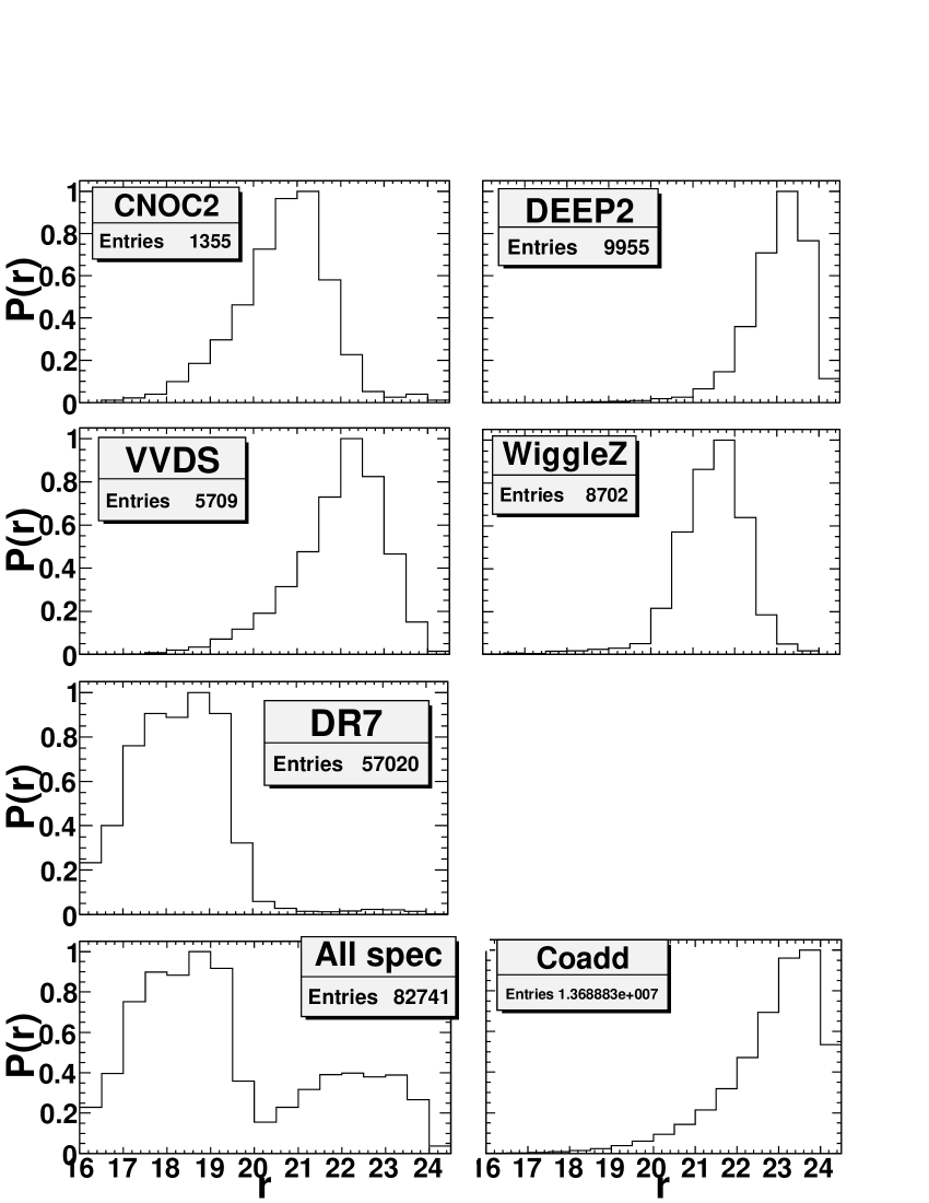
Figure 1: Normalized $r$ magnitude distributions for various catalogs. Top three rows: the distributions of the spectroscopic catalogs used for photo-z training and validation are shown for CNOC2, DEEP2, VVDS, WiggleZ and SDSS DR7. $Entries$ denotes the number of unique galaxy measurements used from each catalog. Bottom left: distribution for the whole spectroscopic sample. Bottom right: the distribution for the SDSS coadd galaxy sample, where objects were classified as galaxies according to the photometric TYPE flag (see text).

The SDSS database provides a variety of measured magnitudes for each detected object. Throughout this paper, we use dereddened model magnitudes to perform the photometric redshift computations. To determine the model magnitude, the SDSS photometric pipeline fits two models to the image of each galaxy in each passband: a de Vaucouleurs (early-type) and an exponential (late-type) light profile. The models are convolved with the estimated point spread function (PSF), with arbitrary axis ratio and position angle. The best-fit model in the $r$ band (which is used to fix the model scale radius) is then applied to the other passbands and convolved with the passband-dependent PSFs to yield the model magnitudes. Model magnitudes provide an unbiased color estimate in the absence of color gradients (Stoughton et al. 2002), and the dereddening procedure removes the effect of Galactic extinction (Schlegel et al. 1998).

Table 1: SDSS Coadd Properties

AB magnitude limits
$u$	23.25
$g$	23.51
$r$	23.26
$i$	22.69
$z$	21.27

Note. — Magnitude limits are for 50% completeness for galaxies in typical seeing (Annis et al. 2011). The median seeing for the SDSS imaging survey is $1.4^{\prime\prime}$.

To construct the photometric sample of galaxies for which we wish to estimate photo-z’s, we obtained a catalog drawn from the SDSS CasJobs website. We checked some of the SDSS photometric flags to ensure that we have obtained a reasonably clean galaxy sample. In particular, we selected all primary objects from Stripe82 that have the TYPE flag equal to $3$ (the type for galaxy) and that do not have any of the flags BRIGHT, SATURATED, or SATUR_CENTER set. For the definitions of these flags we refer the reader to the PHOTO flags entry at the SDSS website or to Appendix A. We also took into account the nominal SDSS coadd flux limit by only selecting galaxies with dereddened model magnitude $r<24.5$. In addition, the co-addition does not propagate information on saturated pixels in individuals runs, and therefore the photometry of objects brighter than $r=15.5$ is suspect. To circumvent this issue we selected only galaxies with $r>16$. The full database query we used is given in Appendix A.

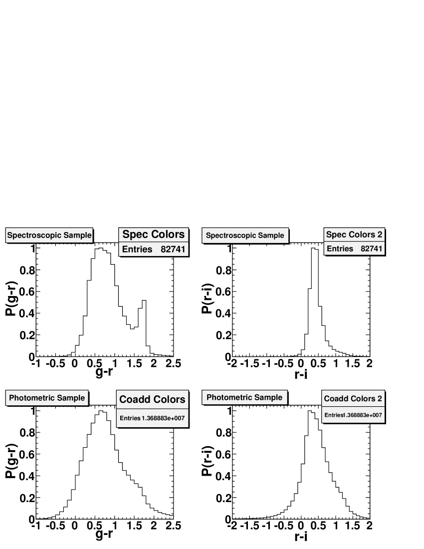
Figure 2: Normalized distribution of $g-r$ and $r-i$ colors. Top row: the color distributions for galaxies in the full spectroscopic sample. Bottom row: the color distributions for galaxies in the photometric sample. As above, galaxy classification used the photometric TYPE flag.

The final photometric sample comprises $13,688,828$ galaxies. Only $2,267$ objects are in DR6 photometric redshift catalog from Oyaizu et al. (2008a). The $r$ magnitude distribution of this sample is shown in the bottom right panel of Fig. 1; the $g-r$ and $r-i$ color distributions are shown in the bottom panels of Fig. 2.

3 Spectroscopic Training and Validation sets

Since our methods to estimate photo-z’s and photo-z errors are training-set based, we would ideally like the spectroscopic training set to be fully representative of the photometric sample to be analyzed, i.e., to have similar statistical properties and magnitude/redshift distributions. Training-set methods can be thought of as inherently Bayesian, in the sense that the training-set distributions form effective priors for the analysis of the photometric sample; to the extent that the training-set distributions reflect those of the photometric sample, we may expect the photo-z estimates to be unbiased (or at least they will not be biased by the prior). Given the practical difficulties of carrying out spectroscopy at faint magnitudes and low surface brightness, such an ideal generally cannot be achieved. Realistically, all we can hope for is a training set that (a) is large enough that statistical fluctuations are small and (b) spans the same magnitude, color, and redshift ranges as the photometric sample (Oyaizu et al. 2008a).

We have constructed a spectroscopic sample consisting of $82,741$ galaxies that have SDSS coadd photometry measurements and that have spectroscopic redshifts measured by the SDSS or by other surveys, as described below. We imposed a magnitude limit of $16<r<24.5$ on the spectroscopic sample and applied additional cuts on the quality of the spectroscopic redshifts reported by the different surveys. Each survey providing spectroscopic redshifts defines a redshift quality indicator; we refer the reader to the respective publications listed below for their precise definitions. For each survey, we chose a redshift quality cut roughly corresponding to 90% redshift confidence or greater. The SDSS spectroscopic sample provides $57,020$ redshifts with confidence level $z_{\rm conf}>0.9$. The remaining redshifts are: $1,355$ from the Canadian Network for Observational Cosmology Field Galaxy Survey (CNOC2; Yee et al. 2000), $9,955$ from the Deep Extragalactic Evolutionary Probe (DEEP2) (Weiner et al. 2005) with $z_{\rm quality}\geq 3$, $8,702$ from the WiggleZ Dark Energy Survey (Drinkwater et al. 2010) with $QoP>3$, $5,709$ from the VIsible imaging Multi-Object Spectrograph - Very Large Telescope Deep Survey (VVDS) (Garilli et al. 2008) with flag $3$ and $4$.

The spectroscopic sample obtained by combining all these catalogs was divided into two catalogs of the same size ($\sim 42,000$ objects each). One of these catalogs was taken to be the training set used by the photo-z and error estimators, and the other was used as a validation set to carry out tests of photo-z quality (see §4.1).

The $r$-magnitude distributions for each spectroscopic sample are shown in Fig. 1, while Fig. 2 shows the color ($g-r$ and $r-i$) distributions for all objects in the final spectroscopic sample. As for how representative the spectroscopic training and validation sample are for the full photometric sample, we checked that the color/magnitude space is fully covered by the spectroscopic sample up to redshift $0.75$ - $0.8$. Beyond this redshift range, the spectroscopic sample partially cover the color/magnitude space. Therefore, the reader need to be cautious when using photo-z’s beyond this range.

4 Methods

4.1 ANN Photometric redshifts

The ANN method that we use to estimate galaxy photo-z’s is a general classification and interpolation tool used successfully in a variety of fields. We use a particular type of ANN called a Feed Forward Multilayer Perceptron to map the relationship between photometric observables and redshifts, as implemented in Oyaizu et al. (2008a).

In this work we use $X$:15:15:15:1 networks to estimate photo-z’s, where $X$ is the number of input photometric parameters per galaxy, following the notation of Collister & Lahav (2004). The corresponding number of degrees of freedom (the number of weights) is roughly 1,000, depending on the actual value of $X$.

Following Oyaizu et al. (2008a), in order to avoid over-fitting, the spectroscopic sample is divided into two independent subsets, the training and validation sets, and the formal minimizations are done using the training set. After each minimization step, the network is evaluated on the validation set, and the set of weights that performs best on the validation set is chosen as the final set. To reduce the chance of ending in a less-than-optimal local minimum, we minimize five networks starting at different positions in the space of weights. Among these, we choose the network that gives the lowest photo-z scatter in the validation set.

We calculated photo-z’s using galaxy magnitudes, colors, and the concentration indices for all passbands. The concentration index $c_{i}$ in a passband $i$ is defined as the ratio of PetroR50 and PetroR90, which are the radii that encircle 50% and 90% of the Petrosian flux, respectively. Early-type (E and S0) galaxies, with centrally peaked surface brightness profiles, tend to have low values of the concentration index, while late-type spirals, with quasi-exponential light profiles, typically have higher values of $c$. Previous studies (Morgan 1958; Shimasaku et al. 2001; Yamauchi et al. 2005; Park & Choi 2005) have shown that the concentration parameter correlates well with galaxy morphological type, and we used it to help break the degeneracy between redshift and galaxy type. We present the photo-z results for different combinations of input parameters in §5.

4.2 Photometric redshift errors

We estimated photo-z errors for objects in the photometric catalog using the Nearest Neighbor Error (NNE) estimator (Oyaizu et al. 2008b), publicly available. The NNE method is training-set based, with a neighbor selection similar to the NNP photo-z estimator; it associates photo-z errors to photometric objects by considering the errors for objects with similar multi-band magnitudes in the validation set. We use the validation set, because the photo-z’s of the training set could be over-fit, which would result in NNE underestimating the photo-z errors. In studies of photo-z error estimators applied to mock and real galaxy catalogs, Oyaizu et al. (2008b) found that NNE accurately predicts the photo-z error when the training set is representative of the photometric sample. In the following, $\sigma^{NNE}_{z}$ will denote the nearest neighbors error estimate.

5 Results

To test the quality of the photo-z estimates, we use the photo-z bias $z_{bias}$ and the photo-z RMS scatter, $\sigma$, defined by

$$z_{bias}=\frac{1}{N}\sum^{N}_{i=1}(z_{phot,i}-z_{spec,i}),$$ (1)

$$\sigma^{2}=\frac{1}{N}\sum^{N}_{i=1}(z_{phot,i}-z_{spec,i})^{2},$$ (2)

and $\sigma_{68}$, the range containing 68% of the validation set objects in the distribution of $\delta z=z_{phot,i}-z_{spec,i}$. In other words, $\sigma_{68}$ is the value of $|z_{phot,i}-z_{spec,i}|$ such that 68% of the objects have $|z_{phot,i}-z_{spec,i}|<\sigma_{68}$. Naturally, if the probability distribution function $P(\delta z)$ is Gaussian $\sigma$ and $\sigma_{68}$ coincide. We also consider $\sigma_{95}$, defined in analogous way.

We computed photo-z’s using the ANN method with different combinations of input photometric observables. All tested combinations are listed in Table 2. In case M, we use the five magnitudes $ugriz$. In case C, we use the four colors $u-g$, $g-r$, $r-i$ and $i-z$. In case CC, we use the four colors with the concentration indices $c_{u}c_{g}c_{r}c_{i}c_{z}$. We also repeat the cases M, C and CC splitting the training set and the photometric sample into 4 bins of $r$ magnitude, $r\leq 18$, $18<r\leq 20$, $20<r\leq 22$, $22<r\leq 24.5$, and perform separate ANN fits in each bin. These cases are dubbed Msplit, Csplit and CCsplit, respectively. For all cases we use the same network configuration, described in Section 4.1.

In Fig. 3 we plot the photometric redshift, $z_{phot}$, for 10,000 randomly selected objects from validation set vs. true spectroscopic redshift, $z_{spec}$, for all considered cases. In each panel, the solid line traces $z_{phot}=z_{spec}$ and the dashed and dotted lines show the corresponding 68% and 95% regions ($\sigma_{68}$ and $\sigma_{95}$), respectively, defined in $z_{spec}$ bins. We find that all cases produce very similar results, in agreement with Oyaizu et al. (2008a).

Table 3 shows a summary of the performance results of the different ANN cases. The standard deviation in this values, estimated from the five networks mentioned in Section 4.1, is $0.001$. We also show in Figure 4 the performance indicators $\sigma$ and $\sigma_{68}$ as functions of $r$ magnitude for all cases. We see that the photo-z scatter increases considerably for $r>22$. This effect can be explained by the small number of objects in the training set covering this regime (see Figure 1). In addition, we show in Figs. 5 and 7 $z_{bias}$, $\sigma$ and $\sigma_{68}$ as functions of estimated photo-z and, in Figs. 6 and 8, the same indicators as functions of the the spectroscopic redshift. We can see that the values of these indicators increase for $z_{phot}>0.75$ regardless the case considered. We show in Table 4 another important indicator, the fraction of catastrophic results, here defined as the number of objects for which we get $|z_{phot}-z_{spec}|>0.1$ divided by the total number in the sample. This definition corresponds to $\sim$ 12 % of the distribution of $|z_{phot}-z_{spec}|$ for this sample. Based on theses results we choose Msplit as the best case. Specifically, Msplit has overall smaller $\sigma_{68}$ as a function of magnitude (Figure 4) and a better fraction of catastrophic results (Table 4).

In Fig. 9 we plot the colors $u-g$, $g-r$, $r-i$ and $i-z$ versus spectroscopic redshift bright ($r<22$) and faint ($r\geq 22$) galaxies in the validation set. We see that, for faint galaxies, colors and spectroscopic redshit are barely correlated. Such degeneracy explains the low efficiency of the method in this magnitude regime.

In Fig. 10 we plot the normalized error distribution, i.e., the distribution of $(z_{phot}-z_{spec})/\sigma_{z}^{NNE}$, for objects in the spectroscopic sample, using the Msplit case, in $r$ magnitude slices, without any bias correction. The solid lines show Gaussian distributions with zero mean and unit variance. These plots indicate that, on average, the photo-z estimates are nearly unbiased and the NNE error is a good estimate of the true error, although we can see some asymmetry in the distribution depending on the magnitude range.

In Fig. 11 we show the distribution of the estimated photometric redshift, corrected for the bias, $z_{phot}-z_{bias}$ for the photometric sample, in $r$ magnitude bins, for our best case (Msplit). The bias was estimated from the validation sample in photo-z bins with width $0.04$ as in Fig. 5. The bias correction is included in the final catalog.

For a significant fraction of the photometric sample the nearest neighbors error estimate is large (greater than 10% of photo-z value) and for most of the science cases it will be necessary to cut the catalog. We show in Fig. 12, the photo-z distributions for the whole sample (as in Fig. 11) and for objects with $\sigma_{z}^{NNE}<0.1$. We also show in Fig. 13 the photometric redshift, $z_{phot}$, for 10,000 randomly selected objects from validation set vs. true spectroscopic redshift, $z_{spec}$ for the same low error subsample.

We found that the use of concentration parameters does not improve significantly the result, in contrast to our initial expectation, based on the SDSS DR6 results (Oyaizu et al. 2008b). O’Mill et al. (2011) also found that these parameters improve the results for the SDSS DR7 main data. This is related to the error in the measured moments for higher magnitudes, which is specially important for this sample, consequently the additional noise roughly compensates the additional information from these parameters. Similar conclusions can be found in (Singalet al. 2011), although their definition of concentration is not the same used here.

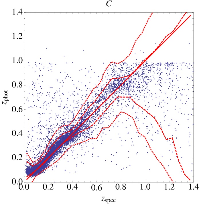
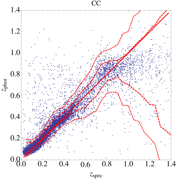
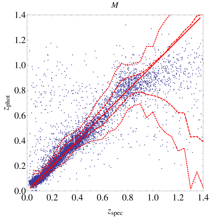
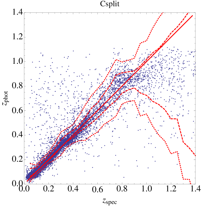
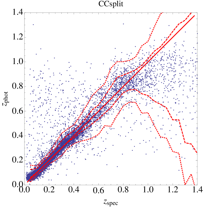
Figure 3: $z_{\rm phot}$ versus $z_{\rm spec}$ for the validation set for different spectroscopic sets and different choices of photometric observables. Top Left: Case C, where the input photometric data comprise the 4 colors ($u-g$, $g-r$, $r-i$, $i-z$) Top Middle: Case CC, where the input data are the 4 colors $u-g$, $g-r$, $r-i$, $i-z$, and 5 concentration parameters $c_{u}c_{g}c_{r}c_{i}c_{z}$. Top Right: Case M, where we use only magnitudes. Bottom Left: Case Csplit, where we split the sample in $r$ magnitude slices. Bottom Middle: Case CCsplit, where we split the sample in $r$ magnitude slices. Bottom Right: Case Msplit, where we split the sample in $r$ magnitude slices. The solid line in each panel indicates $z_{\rm phot}=z_{\rm spec}$; the dashed and dotted lines show the 68% and 95% confidence regions as a function of $z_{\rm spec}$ ($\sigma_{68}$ and $\sigma_{95}$), respectively. The points display results for a random $10,000$ objects subset of the validation set.

Table 2: Description of the different combinations

Case	Inputs/Description
C	$u-g$, $g-r$, $r-i$, $i-z$
Csplit	$u-g$, $g-r$, $r-i$, $i-z$, split in $r$ slices
M	$u$, $g$, $r$, $i$, $z$
Msplit	$u$, $g$, $r$, $i$, $z$, split in $r$ slices
CC	$u-g$, $g-r$, $r-i$, $i-z$ + $c_{u},c_{g},c_{r},c_{i},c_{z}$
CCsplit	$u-g$, $g-r$, $r-i$, $i-z$ + $c_{u},c_{g},c_{r},c_{i},c_{z}$, split in $r$ slices

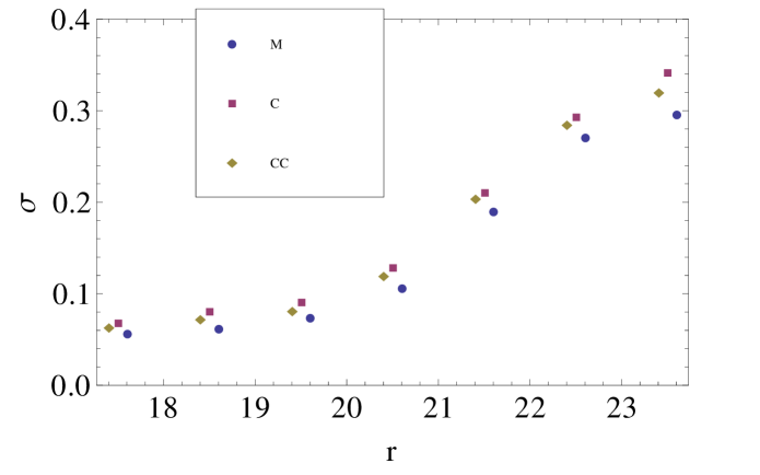
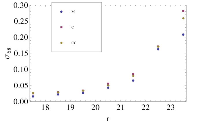
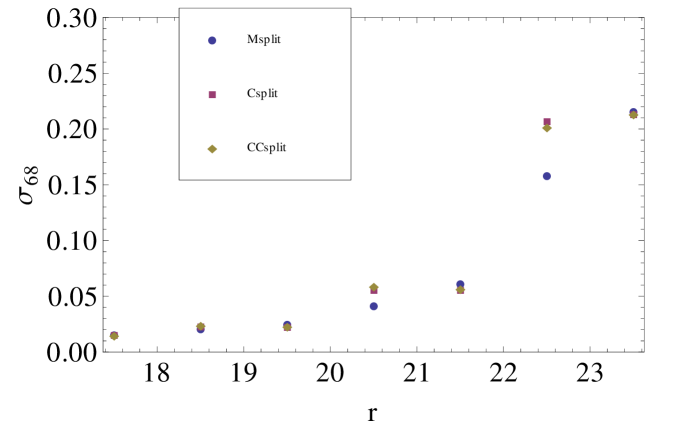
Figure 4: $\sigma$ and $\sigma_{68}$ as functions of $r$ magnitude for all tested cases.

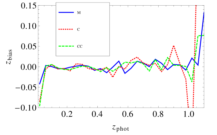
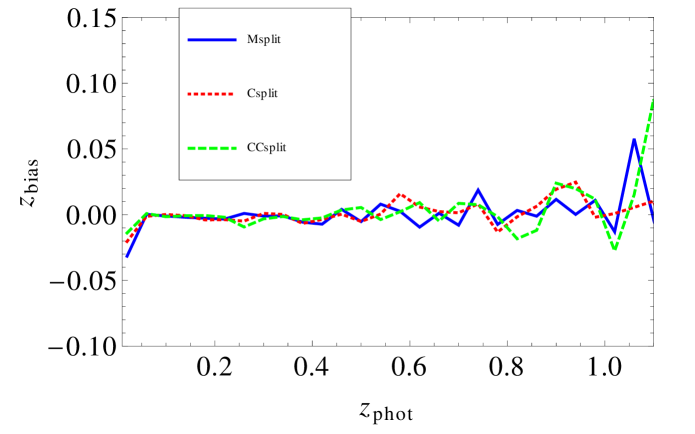
Figure 5: $z_{bias}$ as a function of the photometric redshift for all tested cases.

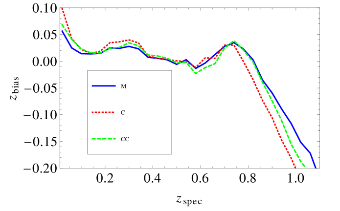
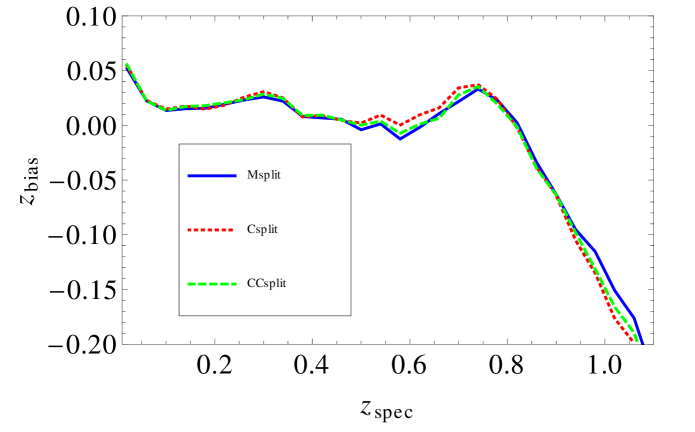
Figure 6: $z_{bias}$ as a function of the spectroscopic redshift for all tested cases.

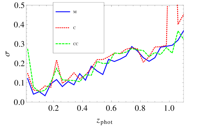
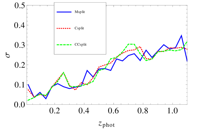
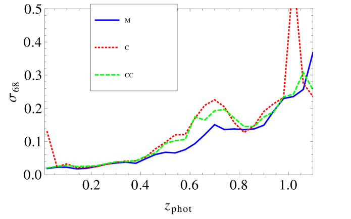
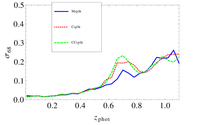
Figure 7: $\sigma$ and $\sigma_{68}$ as a function of the photometric redshift for all tested cases.

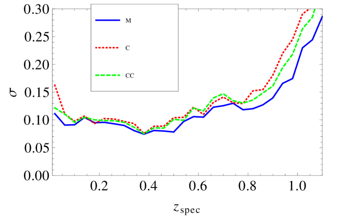
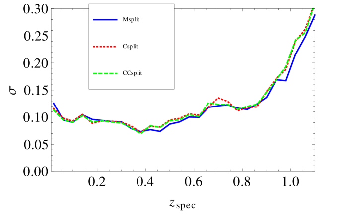
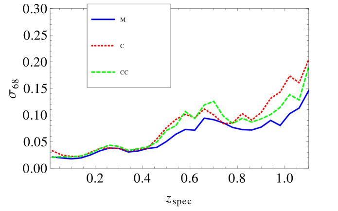
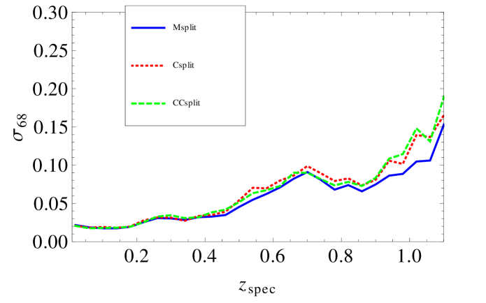
Figure 8: $\sigma$ and $\sigma_{68}$ as a function of the spectroscopic redshift for all tested cases.

Table 3: Summary of ANN cases

Case	$\sigma$	$\sigma_{68}$
C	0.16	0.046
Csplit	0.14	0.034
M	0.14	0.034
Msplit	0.14	0.031
CC	0.15	0.043
CCsplit	0.14	0.032

Note. — $\sigma$ and $\sigma_{68}$ for the validation set using different input parameters (magnitudes, colors, and concentration indices) and training procedures (training with the whole sample or in magnitude bins independently).

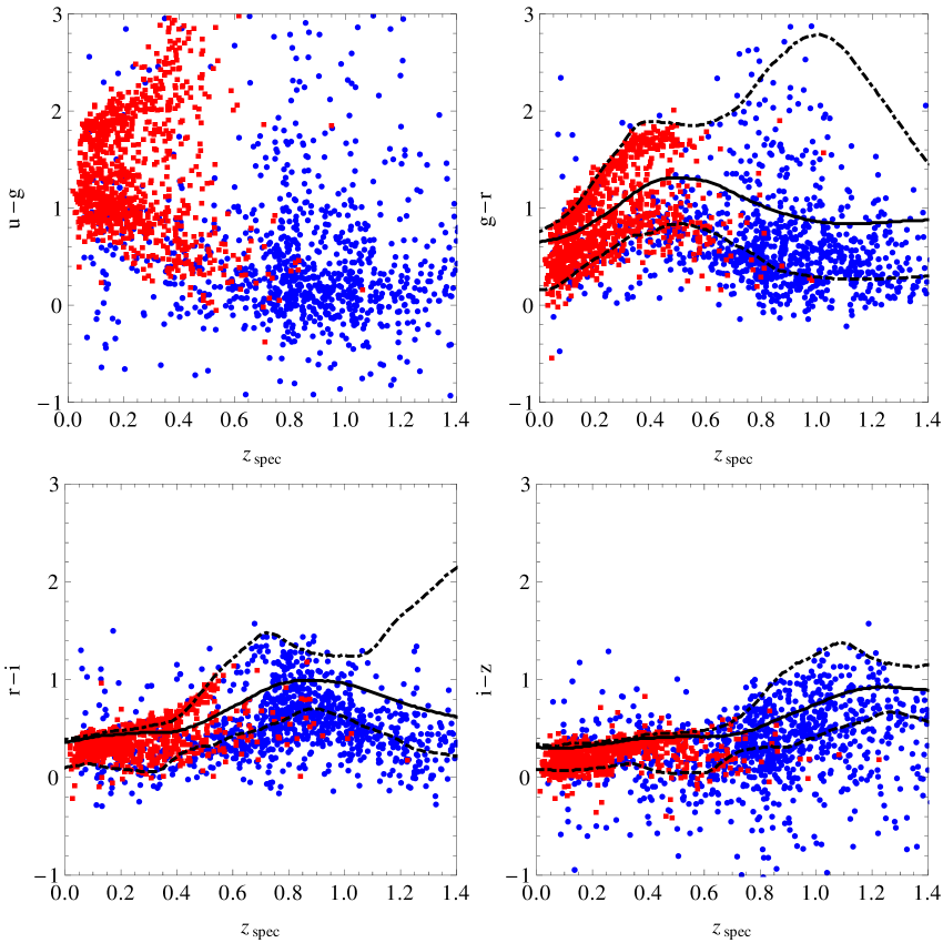
Figure 9: Colors vs spectroscopic redshift for galaxies in the validation set. Red squares (blue circles) denote galaxies with $r<22$ ($r\geq 22$). The curves are the predicted color-redshift relations for different types of galaxies (E,Sbc,Im) obtained by redshifting the k-corrected SEDs of Assef et al. (2010) and applying the appropriate filters.

Table 4: Catastrophic redshifts

	$r<18$	$18<r<19$	$19<r<20$	$20<r<21$	$21<r<22$	$22<r<23$	$r>23$	all
C	0.020	0.034	0.048	0.092	0.14	0.22	0.17	0.075
Csplit	0.0013	0.0063	0.0058	0.093	0.084	0.28	0.29	0.062
M	0.0012	0.0034	0.012	0.054	0.10	0.26	0.26	0.058
Msplit	0.0012	0.0042	0.0068	0.059	0.11	0.25	0.24	0.055
CC	0.013	0.022	0.030	0.066	0.13	0.25	0.21	0.069
CCsplit	0.0012	0.0053	0.0056	0.089	0.083	0.28	0.28	0.060

Note. — Fraction of objects ($N_{cat}/N_{total}$) with $|z_{phot}-z_{spec}|>0.1$ for the validation set using different input parameters (colors, concentration indices and magnitudes) and training procedures.

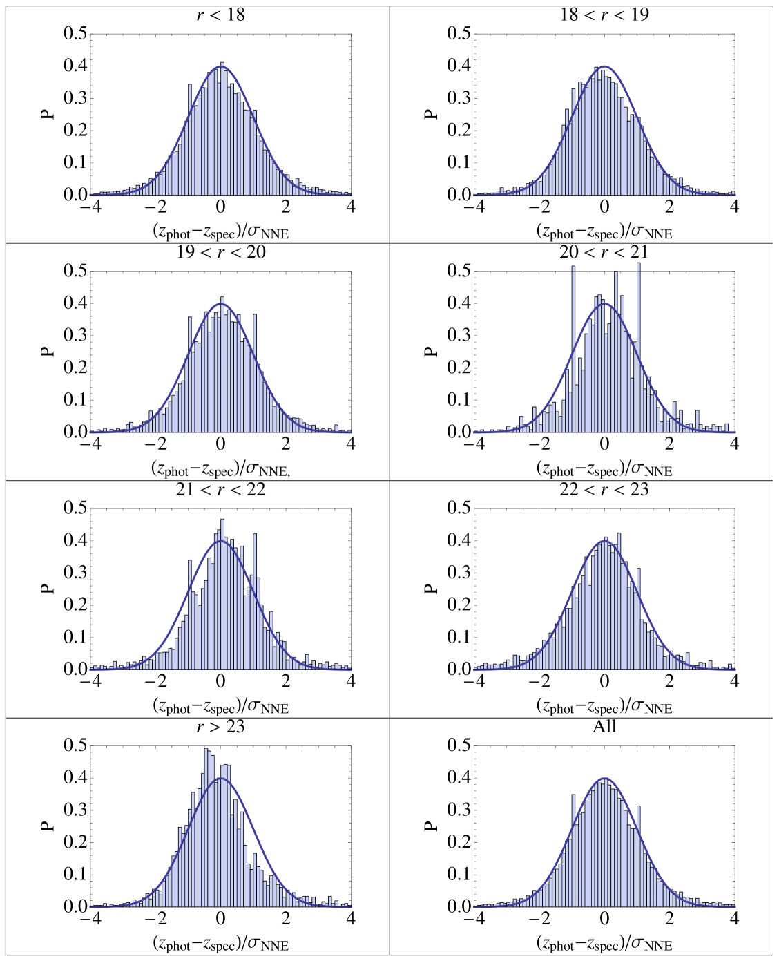
Figure 10: Distributions of $(z_{phot}-z_{spec})/\sigma_{z}^{NNE}$ for objects in the spectroscopic sample, in $r$ magnitude slices, for the Msplit case.

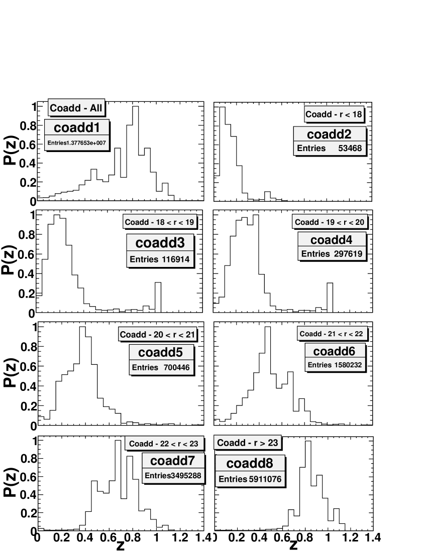
Figure 11: Photometric redshift distributions, corrected for bias, in $r$ magnitude slice for the case Msplit.

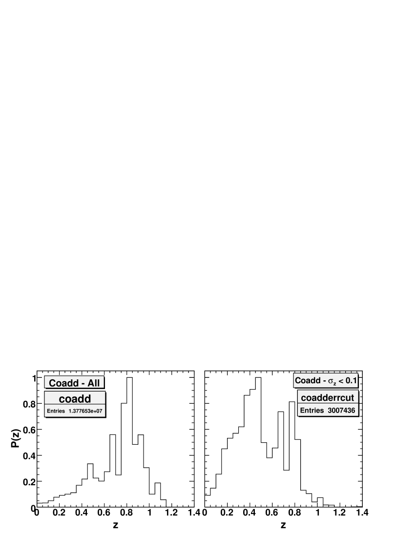
Figure 12: Photometric redshift distributions, for the case Msplit. Left: All objects. Right: Objects with $\sigma_{z}^{NNE}<0.1$.

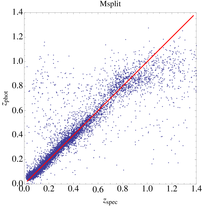
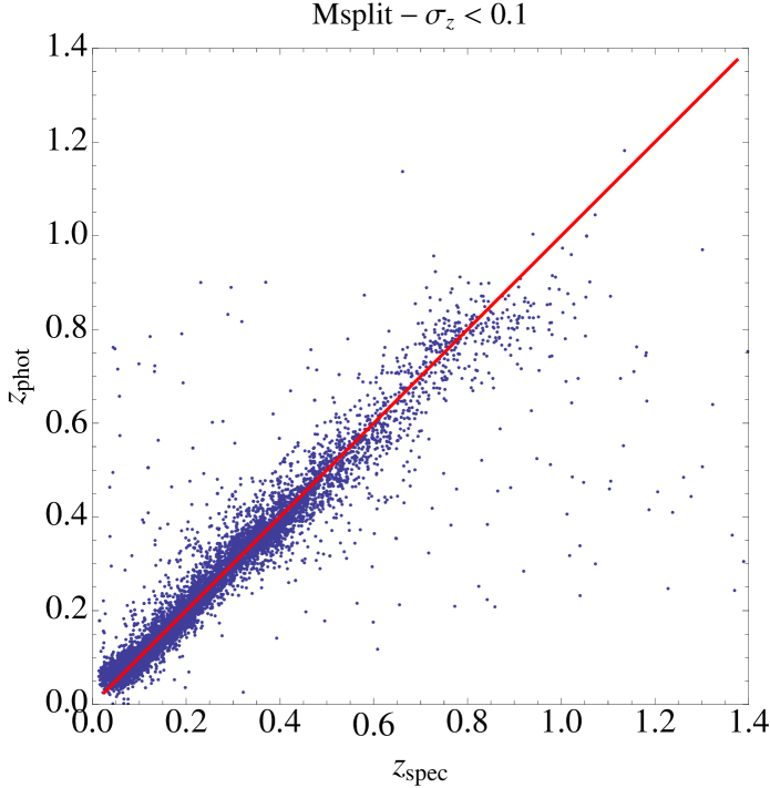
Figure 13: Photo-z vs. spectroscopic redshift for Msplit case. Left: Full sample as in Fig. 3. Right: Only objects with $\sigma_{z}^{NNE}<0.1$.

6 Accessing the Catalog

The best case bias corrected photo-z catalog (Msplit) is publicly available as a SDSS value-added catalog at http://www.sdss.org/dr7/products/value_ added/index.html.

7 Conclusions

We have presented a public catalog of photometric redshifts for the SDSS coadd photometric sample using photo-z estimates, based on the ANN method, considering the five magnitudes $ugriz$ as input parameters and also performing the training in $r$ magnitude bins separately (Msplit). Our tests indicate that the photo-z estimates are most reliable for galaxies with $r<22$ and that the scatter increases significantly at fainter magnitudes. Based on our results, we advise the reader to use carefully this catalog for $z_{phot}\geq 0.75$, since all performance indicators show a lower efficiency of the method, with the chosen spectroscopic sample, at this redshift range. However, depending on the specific science goals, a simple quality cut on the photo-z error might be sufficient to compensate this problem at the desired level.

Appendix A Data Query Code

Here we provide the SDSS database query used to obtain the catalog containing the photometric sample used in this paper. Notice that the query requires the TYPE flag to be set to 3 (galaxies) and selects objects with dereddened model magnitude $16<r<24.5$, which do not have any of the following flags: BRIGHT, SATURATED and SATUR_CENTER. The full query is shown below

SELECT  ObjID,ra,dec,
        dered_u,dered_g,dered_r,dered_i,dered_z,
        petroR50_u/petroR90_u as c_u,petroR50_g/petroR90_g as c_g,
        petroR50_r/petroR90_r as c_r,
        petroR50_i/petroR90_i as c_i,petroR50_z/petroR90_z as c_z,
        err_u,err_g,err_r,err_i,err_z
INTO coadd_mags_allinone
FROM Stripe82..PhotoObjAll
WHERE (flags_r & 0x0000080000040002)=0
        AND type=3
        AND mode=1
        AND (run=106 or run=206)
        AND dered_r BETWEEN 16 AND 24.5

We made an additional cut in order to select only objects which have positive values for petroR50/petroR90. The final catalog has 13,688,828 galaxies.

Here we provide a brief description of the flags used in the query: BRIGHT indicates that an object is a duplicate detection of an object with signal to noise greater than $200\sigma$; SATURATED indicates that an object contains one or more saturated pixels; SATUR_CENTER indicates that the object center is close to at least one saturated pixel. Note that in selecting PRIMARY objects (using PhotoPrimary), we have implicitly selected objects that either do not have the BLENDED flag set or else have NODEBLEND set or nchild equal zero. In addition, the PRIMARY catalog contains no BRIGHT objects, so the cut on BRIGHT objects in the query above is in fact redundant. BLENDED objects have multiple peaks detected within them, which PHOTO attempts to deblend into several CHILD objects. NODEBLEND objects are BLENDED but no deblending was attempted on them, because they are either too close to an EDGE, or too large, or one of their children overlaps an edge. A few percent of the objects in our photometric sample have NODEBLEND set; some users may wish to remove them.

We also suggest that users require objects to have the BINNED1 flag set. BINNED1 objects were detected at $\geq 5\sigma$ significance in the original imaging frame.

The SDSS webpage provides further recommendations about flags, which we strongly recommend that users read.

References

- Abazajian et al. (2009) Abazajian, K. et al. 2009, ApJS, 182, 543
- Annis et al. (2011) Annis, J. et al. 2011, arXiv:1111.6619
- Assef et al. (2010) Assef, J. et al. 2010, ApJ, 713, 970
- Blanton et al. (2003) Blanton, M. R., Lin, H., Lupton, R. H., Maley, F. M., Young, N., Zehavi, I., & Loveday, J. 2003, AJ, 125, 2276
- Cannon et al. (2006) Cannon, R. et al. 2006, MNRAS, 372, 425
- Coleman et al. (1980) Coleman, G. D., Wu, C. C., & Weedman, D. W. 1980, ApJS, 43, 393
- Collister & Lahav (2004) Collister, A. A. & Lahav, O. 2004, PASP, 116, 345
- Connolly et al. (1995) Connolly, A. J. et al. 1995, AJ, 110, 2655
- Csabai et al. (2003) Csabai, I. et al. 2003, AJ, 125, 580
- d’Abrusco et al. (2007) d’Abrusco, R. et al. 2007, ArXiv Astrophysics e-prints, 0701137
- Drinkwater et al. (2010) Drinkwater, M. J. et al. 2010, MNRAS, 401, 1429
- Eisenstein et al. (2001) Eisenstein, D. J. et al. 2001, AJ, 122, 2267
- Fukugita et al. (1996) Fukugita, M., Ichikawa, T., Gunn, J. E., Doi, M., Shimasaku, K., & Schneider, D. P. 1996, AJ, 111, 1748
- Garilli et al. (2008) Garilli, B. et al. 2008, A&A, 486, 683
- Gunn et al. (1998) Gunn, J. E. et al. 1998, AJ, 116, 3040
- Gunn et al. (2006) —. 2006, AJ, 131, 2332
- Hogg et al. (2001) Hogg, D. W., Finkbeiner, D. P., Schlegel, D. J., & Gunn, J. E. 2001, AJ, 122, 2129
- Ivezić et al. (2004) Ivezić, Ž. et al. 2004, Astronomische Nachrichten, 325, 583
- Jiang et al. (2008) Jiang, L. et al. 208, AJ, 135, 1057
- Lupton et al. (2001) Lupton, R., Gunn, J. E., Ivezić, Z., Knapp, G. R., & Kent, S. 2001, in ASP Conf. Ser. 238: Astronomical Data Analysis Software and Systems X, ed. F. R. Harnden, Jr., F. A. Primini, & H. E. Payne, 269
- Morgan (1958) Morgan, W. W. 1958, PASP, 70, 364
- O’Mill et al. (2011) O’Mill, A. L. 2011, MNRAS, 413, 1395
- Oyaizu et al. (2008a) Oyaizu, H., Lima, M., Cunha, C., Lin, H., Frieman, J., & Sheldon E. S. 2008 ApJ674, 768
- Oyaizu et al. (2008b) Oyaizu, H., Lima, M., Cunha, C., Lin, H., & Frieman, J. 2008 ApJ689, 709
- Park & Choi (2005) Park, C. & Choi, Y.-Y. 2005, ApJ, 635, L29
- Pier et al. (2003) Pier, J. R. et al. 2003, AJ, 125, 1559
- Schlegel et al. (1998) Schlegel, D. J., Finkbeiner, D. P., & Davis, M. 1998, ApJ, 500, 525
- Shimasaku et al. (2001) Shimasaku, K. et al. 2001, AJ, 122, 1238
- Singalet al. (2011) Singal, J. et al. 2011, PASP, 123, 615
- Smith et al. (2002) Smith, J. A. et al. 2002, AJ, 123, 2121
- Stoughton et al. (2002) Stoughton, C. et al. 2002, AJ, 123, 485
- Strauss et al. (2002) Strauss, M. A. et al. 2002, AJ, 124, 1810
- Tucker et al. (2006) Tucker, D. L. et al. 2006, Astronomische Nachrichten, 327, 821
- Vanzella et al. (2004) Vanzella, E. et al. 2004, A&A, 423, 761
- Wadadekar (2005) Wadadekar, Y. 2005, Publ. Astron. Soc. Pac., 117, 79
- Weiner et al. (2005) Weiner, B. J. et al. 2005, ApJ, 620, 595
- Yamauchi et al. (2005) Yamauchi, C. et al. 2005, AJ, 130, 1545
- Yee et al. (2000) Yee, H. K. C. et al. 2000, ApJS, 129, 475
- York et al. (2000) York, D. G. et al. 2000, AJ, 120, 1579