Tidal Signatures in the Faintest Milky Way Satellites: The Detailed Properties of Leo V, Pisces II and Canes Venatici II

Abstract

We present deep wide-field photometry of three recently discovered faint Milky Way satellites: Leo V, Pisces II, and Canes Venatici II. Our main goals are to study the structure and star formation history of these dwarfs; we also search for signs of tidal disturbance. The three satellites have similar half-light radii ($\sim 60-90$ pc) but a wide range of ellipticities. Both Leo V and CVn II show hints of stream-like overdensities at large radii. An analysis of the satellite color-magnitude diagrams shows that all three objects are old ($>$ 10 Gyr) and metal-poor ([Fe/H] $\sim-2$), though neither the models nor the data have sufficient precision to assess when the satellites formed with respect to cosmic reionization. The lack of an observed younger stellar population ($\lesssim 10$ Gyr) possibly sets them apart from the other satellites at Galactocentric distances $\gtrsim 150$ kpc. We present a new compilation of structural data for all Milky Way satellite galaxies and use it to compare the properties of classical dwarfs to the ultra-faints. The ellipticity distribution of the two groups is consistent at the $\sim$2-$\sigma$ level. However, the faintest satellites tend to be more aligned toward the Galactic center, and those satellites with the highest ellipticity ($\gtrsim 0.4$) have orientations ($\Delta\theta_{GC}$) in the range $20^{\circ}\lesssim\Delta\theta_{GC}\lesssim 40^{\circ}$. This latter observation is in rough agreement with predictions from simulations of dwarf galaxies that have lost a significant fraction of their dark matter halos and are being tidally stripped.

1. Introduction

By detecting slight over-densities of stars with the appropriate color and magnitude in the Sloan Digital Sky Survey (SDSS) catalogs, over 15 new, faint satellites have been discovered around the Milky Way (MW) in the last eight years (Willman et al. 2005a, b; Zucker et al. 2006a, b; Belokurov et al. 2006, 2007; Irwin et al. 2007; Belokurov et al. 2008, 2009, 2010; Walsh et al. 2007, see Willman (2010) for a recent review). As a population, these objects are less luminous (with $-1.5<M_{V}<-8.6$), and more extended (with $20\lesssim r_{h}\lesssim 220$ pc) than a typical globular cluster. Initial studies of these objects indicate that they are predominantly old, metal poor, and dominated by dark matter (e.g. de Jong et al. 2008b; Kirby et al. 2008; Simon & Geha 2007).

Cold Dark Matter (CDM) simulations predict more than an order of magnitude more DM subhalos orbiting the MW than we see as luminous satellites, a discrepancy that increases with increasing simulation resolution (e.g. Moore et al. 1999; Diemand et al. 2007). However, connecting simulations with observations is not trivial. If the CDM picture is correct, then we can test the physics of galaxy formation by comparing the observed numbers and properties of the MW satellites with the predictions of simulations that incorporate such physics (see e.g. Kravtsov 2010, for a recent review). On the observational side, an in depth understanding of the new satellites’ star formation history (SFH), structure, mass, internal dynamical state and orbital history around the MW are all necessary before we can understand how stars populate the smallest DM halos.

Among the new MW satellites, Canes Venatici II (CVn II), Leo V, and Pisces II are an intriguing triplet with similar properties (see Belokurov et al. 2007, 2008, 2010, for their discovery papers, respectively). They are all very distant from the MW ($D>150$ kpc), have similar half light radii ($50\lesssim r_{h}\lesssim 100$ pc) and are among the faintest objects (with $-4.0\lesssim M_{V}\lesssim-5.0$) detectable in the SDSS at that distance (Koposov et al. 2008; Walsh et al. 2009). Based on spectroscopic results, CVn II appears to be dark matter dominated with a $M/L_{V}=360^{+380}_{-180}$ (Wolf et al. 2010) and is metal poor, with $\langle$[Fe/H]$\rangle=-2.19$ (Kirby et al. 2008). On the other hand, neither Leo V nor Pisces II have robust mass estimates, although the kinematic study of Walker et al. (2009b) suggests that Leo V might be dark matter dominated. Leo V bears several hints that it might have been tidally stripped, including a spectroscopic [Fe/H] that is higher than MW satellites of similar luminosity, and more compatible with brighter objects. Leo V also shows signs of being disturbed, with an apparently extended blue horizontal branch distribution (Belokurov et al. 2008) and kinematic members more then 10 half light radii away from the satellite center (Walker et al. 2009b). There have also been suggestions that Leo V and the nearby satellite Leo IV are connected by a ‘stellar bridge’, and share a common origin (de Jong et al. 2010, but see Sand et al. (2010)). Pisces II has had no published spectroscopic follow up to date.

Their stellar populations, based on earlier work, appears to be uniformly old ($\gtrsim$ 10 Gyr) and metal poor ([Fe/H]$\lesssim-2$), with no obvious sign of more recent star formation. If confirmed, then these three satellites have qualitatively different formation histories than other similarly distant MW satellites. Among the eight classical dSphs, the four with the largest distance from the MW ($D>90$ kpc) all have extended star formation histories (SFHs), with significant amounts of star formation occurring within the last 10 Gyr (Dolphin et al. 2005). The other two faint MW satellites with $D>150$ kpc, Leo IV and CVn I, both have signs of more recent star formation based on an excess number of blue plume stars which appear clumped and segregated within the main body of the satellite (Martin et al. 2008a; Sand et al. 2010, but see Okamoto et al. (2012)).

Motivated by all of the above, we obtained deep, wide-field ($\sim 25^{\prime}\times 25^{\prime}$) photometry of Leo V, CVn II and Pisces II on $\sim$6-8 meter class telescopes, with the goal of ascertaining their structure and star formation history. An outline of the paper follows. In Section 2, we describe the observations, data reduction, photometry and final point source catalogs of our objects. In Section 3 we measure the distance to our satellites (when not already established with RR Lyrae stars in the literature) via the magnitude of their blue horizontal branch (BHB) stars. Section 4 details the structural properties of our three satellites including both a parameterized fit to their ridgeline stars and a matched-filter search for signs of extended/disturbed structure. Section 5 presents a qualitative analysis of each satellite’s SFH, and a measurement of their luminosity. We then take a step back in § 6 to place the three objects in the context of the new MW satellite population as a whole. We compare the structural properties of the new satellites with the classical dSphs, and search for signs of tidal disturbance based on their alignment with the vector to the MW center. Finally, we summarize and conclude in Section 7. Throughout this work, we use the terms ‘ultra-faint satellites’, ‘post-SDSS satellites’ and ‘new MW satellites’ interchangeably to represent the MW satellites discovered via matched-filter techniques of the SDSS point source catalogs.

2. Observations & Data Reduction

Here we describe the observations, data reduction and photometry of Leo V, Pisces II, and CVn II used in this paper. At the end of this section, we present our full Leo V, Pisces II and CVn II photometry catalogs. A summary of the observations is in Table 1.

We observed Leo V on 2010 April 13 (UT) and Pisces II on 2010 Oct 3 (UT) with Megacam (McLeod et al. 2006) on the f/5 focus at the Magellan Clay telescope in the $g$ and $r$ bands. Magellan/Megacam has 36 CCDs, each with $2048\times 4608$ pixels at 0$\farcs$08/pixel (which were binned $2\times 2$), for a total field of view (FOV) of $\sim$24’$\times$24’. We reduced the data identically to Sand et al. (2010) using the Megacam pipeline developed at the Harvard-Smithsonian Center for Astrophysics by M. Conroy, J. Roll and B. McLeod.

Subaru/Suprimecam data of CVn II comes from the SMOKA science archive, which archives the public data of the Subaru Telescope. While other data on CVn II are available, we retrieved the deep $V$ and $I$ imaging observed by Okamoto and collaborators (see Okamoto et al. 2012, for their presentation of their CVn II data), as summarized in Table 1. We have reduced the archival Suprimecam (Miyazaki et al. 2002) data of CVn II in a standard way, performing bias subtraction and flat fielding with the provided calibration frames. Cosmic-ray rejection of each individual exposure was done with the lacosmic task (van Dokkum 2001). An astrometric solution was found via SCAMP using the SDSS-DR7 catalog. Once a good astrometric solution was found, the image resampling and co-addition software SWarp was employed (with the lanczos3 interpolation function) using a weighted average of the individual frames to make our final image stack. Note that we have not included one corner CCD (DET-ID 0) into our final image stacks due to poor charge transfer efficiency at the time of the observations.

We performed stellar photometry on the final image stacks using a methodology identical to that in our previous works (Sand et al. 2009, 2010) with the command line version of the DAOPHOTII/Allstar package (Stetson 1994). Here we briefly reiterate. We allowed for a quadratically varying point spread function (PSF) across the field when determining our model PSF and ran Allstar in two passes – once on the final stacked image and then again on the image with the first round’s stars subtracted, in order to recover fainter sources. We culled our Allstar catalogs of outliers in $\chi^{2}$ versus magnitude, magnitude error versus magnitude and sharpness versus magnitude space to remove objects that were not point sources. We positionally matched our source catalogs derived from different filters with a maximum match radius of 0$\farcs$5, only keeping those point sources detected in both bands in our final catalog.

We converted instrumental magnitudes into the SDSS photometric system using stars in common with SDSS-DR7, as in Sand et al. (2010), which included a color term. For our $V$ and $I$ band observations of CVn II, we used the filter transformations of Jordi et al. (2006) to convert from SDSS catalog magnitudes to $V$ and $I$ bands. Slight residual zeropoint gradients across the FOV were fit to a quadratic function and corrected for (see also Saha et al. 2010), resulting in a final overall scatter about the best fit zeropoint of $\delta\lesssim 0.05$ mag in all of our photometric bands.

We performed a series of artificial star tests to calculate our photometric errors and completeness as a function of magnitude and color for each of our fields. Artificial stars were placed into our images on a regular grid (10 to 20 times the image FWHM), with the DAOPHOT routine ADDSTAR. Ten iterations were performed on each field, yielding between $\sim 6\times 10^{5}$ and $\sim 8\times 10^{5}$ implanted artificial stars. The $r$ ($I$) magnitude for a given artificial star was drawn randomly from 18 to 29 mag, with an exponentially increasing probability toward fainter magnitudes. The $g-r$ ($V-I$) color is then randomly assigned over the range ($-0.5$,1.5) with equal probability. These artificial star frames were then run through the same photometry pipeline as the unaltered science frames, applying the same $\chi^{2}$, sharpness and magnitude-error cuts. The 50% and 90% completeness for each of our fields and imaging bands is summarized in Table 1.

2.1. Final Catalogs and Color Magnitude Diagrams

We present our full Leo V, Pisces II and CVn II catalogs in Tables 2-4. Each table includes the calibrated magnitudes (uncorrected for extinction) with their uncertainty, along with the Galactic extinction values derived for each star (Schlegel et al. 1998). We also note whether the star was taken from the SDSS catalog rather than our Magellan or Subaru photometry, as was done for objects near or brighter than the saturation limit of the observations. All magnitudes reported in the remainder of this paper will be corrected for Galactic extinction.

The color magnitude diagram (CMD) of each of our satellites is presented in Figure 1. Plotted in the left panel are all stars within two half-light radii (as determined in § 4.1), while the right panel is a Hess diagram of the same region with a scaled background subtracted, using stars located outside a radius of 8 arcminutes. We highlight possible stellar populations for each of our satellites in both panels. In the right panels of each satellites’ CMD we plot a theoretical isochrone from Girardi et al. (2004), with [Fe/H]=$-2.0$ and age of 13.5 Gyr, using the satellite distances as determined in § 3. The solid box in the left panels in Figure 1 denotes our initial blue horizontal branch (BHB) star selection region in the CMDs. We study the BHB spatial distribution in each dwarf in § 4.2.

3. Satellite Distances

The distance to each of the satellites is necessary for deriving their physical size and placing them in context with respect to the MW satellite population as a whole.

We constrain the distance to Pisces II and Leo V using the luminosity of their horizontal branch (HB) sequence in the following way. First, two fiducial HB star sequences were constructed using SDSS photometry; one from the globular cluster (GC) M92 and the other from the union of M3 and M13. For clarity in what follows, we assume distance moduli of $\mu=14.75\pm 0.1$, $15.14\pm 0.2$ and $14.31\pm 0.1$ mag for M92 (Kraft & Ivans 2003), M3 (Cho et al. 2005) and M13 (Kraft & Ivans 2003), respectively. The uncertainty in distance modulus for M3 was taken directly from the analysis of Cho et al. (2005), while that for M92 and M13 are estimated based on their agreement with the independent distance measurement of VandenBerg (2000). We note that our value for M92’s distance is $\sim$0.15 mag different from that in the Harris GC catalog (Harris 1996, who report a distance to M92 of 8.3 kpc, or $\mu$=14.6 mag). We take literature values of [Fe/H]=$-$2.4 and E(B-V)=0.022 mag for M92, and [Fe/H]=$-$1.5 and E(B-V)=0.013 mag for M3 and [Fe/H]=$-$1.6 and E(B-V)=0.017 for M13 (Kraft & Ivans 2003).

We then gathered HB stars for Leo V and Pisces II, taking stars out to 2.5$r_{h}$ (see § 4.1), as this is roughly the distance at which there were clear members with no offset from the HB sequence. We fit to both of the GC fiducial HB sequences by minimizing the sum of the squares of the difference between the data and the fiducial, and summarize the results in Table 5. Given the relation between metallicity and HB luminosity (see e.g. Catelan 2009, for a recent review), we also determined distances assuming a nominal [Fe/H]=$-$2.0, given that $M_{V,HB}\propto 0.2\times$[Fe/H], and using the M3/13-derived distance as a baseline. In this case, we added a further uncertainty of 0.05 mag to represent the uncertainty in the $M_{V,HB}-[Fe/H]$ relation. We note that Leo V has a spectroscopic [Fe/H]=$-2.0\pm 0.2$ (Walker et al. 2009a), while Pisces II has no published spectroscopic metallicity.

Uncertainties are calculated via jackknife resampling, which accounts for both the finite number of stars in each satellite, and the possibility of occasional interloper stars. The uncertainties associated with our calibration to the SDSS photometric system ($\lesssim 0.01$ mag), our globular cluster fiducial distance uncertainties, and reddening ($\sim$0.03 mag) were added in quadrature to produce our final quoted uncertainty. The systematic uncertainty associated with the metallicity-luminosity relation of HB stars – which we estimate to be $\sim$0.05 mag – was added to the uncertainty in the distance derived via our M3/M13 translation to [Fe/H]=$-$2.0.

Our M92-derived distance to Leo V is offset from that previously reported using the same cluster as a fiducial in the discovery work of Belokurov et al. (2008), who found D=178 kpc. We suspect that this difference is due to the ambiguity in M92’s distance rather than the Leo V photometry itself, although this cannot be definitively tracked down since it is unclear what distance to M92 Belokurov et al. used. The distance to Pisces II determined in the discovery paper of Belokurov et al. (2010), D$\sim$182 kpc, is consistent with our measurements to that satellite.

Given the ambiguity of M92’s distance, the lack of a spectroscopic [Fe/H] for Pisces II, and the reasonable consistency of their stellar populations with the [Fe/H]=$-$2.0 isochrones (see § 5), we utilize our [Fe/H]=$-$2.0 distance measurements for Leo V and Pisces II for the remainder of this work.

To lend credence to our technique, we have utilized the HB data of Leo IV from Sand et al. (2010), and measured D=158$\pm$12 kpc for a HB with [Fe/H]=$-$2.0, which is in excellent agreement with the RR Lyrae distance, D=154$\pm 5$ kpc, as determined by Moretti et al. (2009). Given this, and a lack of globular cluster fiducials in the $V$ and $I$ band (the photometric bands of our CVn II data), we directly adopt the RR Lyrae distance of CVn II measured by Greco et al. (2008) – $\mu=21.02\pm 0.06$ mag ($160\pm 7$ kpc) – which matches the old stellar population isochrones in Figure 1.

4. Structural Properties

We split our structural analysis into two parts. First, we fit parameterized models to the two dimensional density profile of our satellites in order to measure their basic structural properties such as half light radius ($r_{h}$) and ellipticity. From there, we search for signs of extended structure, such as tidal streams, around each satellite using a matched-filter technique.

4.1. Parameterized Fits

As in previous work on the classical and ultra-faint MW satellites, we fit standard parameterized models – the Plummer and exponential distribution – to the surface density profile of the three objects in the present study. While the observed MW satellites have a complexity and non-uniformity that can not be characterized with parameterized models, it is nonetheless important to quantify their structure in a consistent way for comparison with previous results. We note that we do not report King profile parameters for the three objects in this study, as we have in previous work – due to the small number of stars in each satellite and the additional free parameter in the King model, we did not obtain reliable results (in particular for Leo V and Pisces II).

We use a maximum likelihood (ML) technique for constraining structural parameters (based on the recipe of Martin et al. 2008), identical to that done in Sand et al. (2010). Our slightly modified technique is robust to non-rectangular field of view geometries because all integrals are calculated via Monte Carlo integration – for instance, Eqn. 5 from Martin et al. (2008b). Both the exponential and Plummer profiles have the same set of free parameters – ($\alpha_{0}$, $\delta_{0}$, $\theta$, $\epsilon$, $r_{half}$, $\Sigma_{b}$). In order, these include the central position, $\alpha_{0}$ and $\delta_{0}$, position angle (PA; $\theta$), ellipticity ($\epsilon$), half light radius ($r_{half}$) and background surface density ($\Sigma_{b}$). Uncertainties on structural parameters are determined through 1000 bootstrap resamples, from which a standard deviation is calculated. The stars selected for this analysis are those consistent with the ridgeline (red giant branch, subgiant branch and the main sequence) of each satellite. Briefly, we use a [Fe/H]=$-2.0$, 13.5 Gyr old theoretical isochrone ridgeline (Girardi et al. 2004), for the satellite distance modulus determined in § 3, and placed two selection boundaries at a minimum of 0.1 mag on either side along the $g-r$ axis. These selection regions are increased to match the typical $g-r$ color uncertainty at a given $r$ magnitude when it exceeds 0.1 mag, as determined via our artificial star tests. The choice of ridgeline is not crucial, because old stellar populations in the expected metallicity range all fall within $\sim$0.1 mag of the ridgeline. We impose a faint magnitude limit corresponding to our 50% completeness limit reported in Table 1. Each selection region was visually checked to verify that stars consistent with the visible ridgeline of each satellite were included in this analysis. Note that HB stars are not included in this technique, although we do discuss their spatial distribution further in § 4.2.

Our results are presented in Table 6. We also show one dimensional stellar radial profiles corresponding to our best-fit parameters, along with our binned data, in Figure 2. Despite the fact that we fit structural parameters to the two dimensional distribution of satellite stars, the one-dimensional representation of the fits show satisfactory, but imperfect, agreement. As mentioned earlier, our parameterized models should not be expected to be excellent descriptions of the satellites’ potentially complex structure. Note that the exponential profile fit to Pisces II did not result in a well-defined ellipticity, and thus major axis position angle, although the Plummer profile fit was able to constrain these quantities. Similarly, the half light radius of Leo V, with either parameterization, had a large ($\sim$50%) uncertainty. To illustrate some of the key parameter degeneracies for the exponential profile fit, we show the two-dimensional, marginalized confidence contours for the half light radius, ellipticity and position angle for the three dwarfs in our study in Figure 3.

Recently, Munoz et al. (2011) presented a suite of simulations of low luminosity MW satellites under different observing conditions to determine the dataset quality necessary to measure accurate structural parameters. In particular, in order to get a $\sim$10% measurement of the half light radius, they suggested a field of view at least three times that of the half light radius being measured, greater than 1000 stars in the total sample, and a central density contrast of 20 over the background. The data presented in this paper has a central density contrast of $\sim$10 (see Figure 2), and this may be responsible for our inability to measure half light radii to $\sim$10%.

Overall, our results are in agreement with those in the literature where there is overlap. We measure CVn II to be marginally rounder ($\epsilon=0.39\pm 0.07$) than the structural analysis of Martin et al. (2008b) performed on the shallower SDSS discovery data ($\epsilon=0.52^{+0.10}_{-0.11}$), but otherwise measure similar parameter values considering the uncertainties. CVn II was studied with nearly identical Subaru data as our own by Okamoto et al. (2012), who found the same half light radius as we do, but a smaller ellipticity, $\epsilon$=0.23 (with no associated uncertainty). This can be attributed to the fact that Okamoto et al. measured their ellipticity after binning and smoothing the data, which is known to systematically lower the resulting ellipticity measurement (Martin et al. 2008b). Our derived half light radius is inconsistent with the deep data obtained for the RR Lyrae study done by Greco et al. (2008), who found $\sim 150$ pc, although their measurement is inconsistent with other literature values as well. It is unclear where this discrepancy originates. Leo V and Pisces II have been discovered since the homogenous analysis of Martin et al. (2008b), but our results are broadly consistent with the discovery data of each object (Belokurov et al. 2008, 2010).

4.2. Extended Structure Search

Given the intriguing structural properties of the new MW satellites as a population (e.g. Martin et al. 2008b), and hints that some of the satellites may be tidally disturbed (e.g. Sand et al. 2009; Muñoz et al. 2010), it is worth searching for signs of extended structure, such as streams or other extensions, within our data. We use a matched-filter technique identical in spirit to that of Rockosi et al. (2002), with a well understood ‘signal’ CMD and ‘contamination’ CMD. We refer the reader to Rockosi et al. (2002) for the details of the algorithm. The matched-filter technique, in contrast to simpler star-counting density maps, gives higher weights to stars which have relatively low contamination, such as BHB stars.

To be successful, we must have high-fidelity signal and contamination CMDs. For the purposes of the matched-filter technique, we bin all of our CMDs into $0.15\times 0.15$ color-magnitude bins in what follows. Rather than use stars from the central regions of each satellite for our signal CMD (which will be sparsely populated and will contain background/foreground stars), we use theoretical isochrones which match our observed satellite CMD and are convolved with our well-understood completeness and uncertainty functions. We take our cue from the qualitative stellar population analysis presented in § 5.1. To be specific, we use the testpop program in the StarFISH software suite; a set of programs designed for fitting the star formation history of observed stellar populations (Harris & Zaritsky 2001). The testpop program will take a theoretical isochrone set, convolve it with the photometric completeness and uncertainties of your observations, and produce a realistic, ‘observed’ CMD. For each satellite, we create realistic CMDs populated with 50000 stars as our signal CMD, using a single stellar population with [Fe/H]=$-2.0$ and an age of 13.5 Gyr from the results of Girardi et al. (2004). We show in § 5.1 that this stellar population is consistent with that seen in our three satellites.

For our contamination, background CMD we use all stars at radii larger than 8 arcmin from our satellite galaxies. Given the small size of our satellites, with half light radii $\lesssim$2 arcmin, this should yield a relatively pure background CMD, unless of course our satellites have low density streams or extensions out to these radii. To guard against this, we repeated our analysis with background CMDs taken only from each of the four separate quadrants of our field of view. These spatially distinct background CMDs did not change our final satellite maps significantly, suggesting that there are no streams which we are washing out by including signal into our background contamination filter.

We show our final maps, both raw and spatially smoothed, for each of our satellites in Figure 4. In the top row of Figure 4 we show our raw matched filter maps with 30 arcsecond pixels, with contours showing (5, 6, 7, 10, 15, 20) $\sigma$ regions above the modal value of the map. The main body of the satellite, along with several other overdensities, are visible in each map. The bottom row of Figure 4 show smoothed versions of the raw map. For each of these we have binned our stars into 20 arcsecond pixels and then smoothed our final values using a Gaussian with width 1.5 times that of the pixel size. The mode of the background of these smoothed maps was determined using the MMM routine in IDL. The contours shown in the plot are (3, 4, 5, 6, 7, 10, 15, 20) standard deviations above the modal value of the map, although their interpretation should be taken with a grain of salt, given that the maps were smoothed. The vector arrow in each plot shows the direction to the Milky Way center. We also show the vector to Leo IV in our map of Leo V; the two satellites are projected $\sim$2 degrees apart on the sky, although we see no sign of connection or interaction between the two (see Sand et al. (2010) and de Jong et al. (2010) for further discussion). We discuss possible satellite alignment with the MW in § 6.3.

There are tentative hints of extended structure in our satellite maps. For instance, there are a series of overdensities going from the Northeast to Southwest in the map of Leo V, and from Southeast to West in CVn II, both of which apparently go through the body of the satellite. We have constructed maps of barely resolved galaxies, by taking those objects culled due to their poor DAOPHOT PSF fits (see § 2), and only a couple of compact galaxy groupings are nearly coincident with those in the maps of our satellites in Figure 4. Nonetheless, better star/galaxy separation, perhaps through near infrared photometry or Hubble Space Telescope imaging, will be necessary to definitively ferret out any possible streams in these systems. The surface brightness at the $3-\sigma$ contour level is ($\mu_{g},\mu_{r}$)=(30.4,30.0) and (29.6,29.2) mag arcsec^-2 for Pisces II and Leo V, respectively. CVn II has surface brightness limits of ($\mu_{V},\mu_{I}$)=(30.3,29.6) mag arcsec^-2.

4.2.1 The distribution of BHB stars

We have also overplotted the spatial positions of BHB star candidates onto our maps in Figure 4, which are marked as blue diamonds. Initial BHB star lists were taken from the blue box region in color-magnitude space in Figure 1 for each satellite, which were then further culled of objects which were not clearly on the BHB sequence. This conservative approach may cause us to remove a time-varying RR Lyrae star candidate which truly does belong to a satellite, but does allow us to evaluate the spatial extent of the BHB population with the minimum amount of foreground/background contamination.

As can be seen from Figure 4, the BHB star population is centrally concentrated around each satellite, although BHB stars at large radii are evident. We take a simple approach to determine if our BHB spatial distributions are consistent with the parameterized model fits we derived for our satellites in § 4.1, which utilized stars on the main sequence to red giant branch ridgeline for parameter estimation. We performed Monte Carlo simulations, randomly placing $N_{BHB}$ stars down at radii drawn from our Plummer and exponential models (varying the half light radius according to its uncertainty) and then comparing the median radius of the simulated sample of BHB stars with the observed median.

According to our simulations, the BHB population of Pisces II and CVn II are consistent with the derived parameterized fit to the ridgeline data. However, given our Leo V structural parameters for the Plummer (exponential) profile fit, there is only a 0.4% (0.3%) chance of getting a BHB sample with an observed median radius that is at least as small as that measured for the bulk of Leo V stars – strong evidence that the BHB stars in Leo V are more extended than the fitted profile (see also Belokurov et al. 2008).

Intrigued by the possibility that Leo V may have an extended BHB stellar distribution, and seeking additional evidence, we ran our ML structural analysis code (see § 4.1) directly on our BHB sample. The advantage of using the ML code is that it naturally incorporates a background surface density ($\Sigma_{b}$) into the structural measurement. In this case, we found a half light radius of $r_{h}=2.9\pm 0.8$ arcmin for our BHB stellar sample (assuming an exponential profile), which is $\sim$1.8$\sigma$ discrepant from that found for Leo V’s ridgeline stars. While tantalizing, we can not say definitively that Leo V has an extended BHB stellar distribution.

5. Stellar Population and Luminosity

In this section, we first perform a qualitative analysis to show which single population stellar ages and metallicities are consistent with our three satellite CMDs. We then utilize the structural properties found in § 4.1, and our newly acquired knowledge of the satellites’ stellar population to calculate their absolute magnitudes.

5.1. General Properties

As can be seen from the CMDs within $2r_{h}$ in Figure 1, our data reach between $\sim$0.5 and 1 magnitudes below the main sequence turnoff. Generally, in order to infer a precise age and metallicity of a stellar population, it is essential to have high quality photometry around and below this turnoff (Dolphin 2002). In our case, we are also fundamentally limited by the small number of satellite stars – between $\sim$200-400, depending on the satellite – as inferred from our parameterized structural analysis (§ 4.1). Because of these limitations, we eschew a CMD-fitting approach to inferring star formation history, and opt to qualitatively assess which single age stellar populations are consistent with our CMDs, given a range of metallicities that bracket the measured values in the literature.

For each satellite, we plot a Hess diagram of all stars within $2r_{h}$, subtracting out a scaled background CMD based on stars greater than 8 arcminutes from the satellites’ center (see Figure 5). We overplot single age theoretical isochrones with age = (8,10,12,13.5) Gyr for a [Fe/H] of ($-2.3$,$-2.0$,$-1.5$), using the theoretical isochrone set of Girardi et al. (2004) throughout. The choice of metallicities brackets the mean spectroscopic metallicity measurements of CVnII (Kirby et al. 2008) and Leo V (Walker et al. 2009b), although the dispersion to very low metallicities seen in CVn II can not be modeled since the Girardi et al. (2004) isochrone set has a minimum [Fe/H] of $-2.3$. We also assume that Pisces II has a comparable metallicity as the other two satellites, a relatively safe assumption since all of the new MW satellites studied thus far have spectroscopic $-2.6<$ [Fe/H] $<-2.0$ (Kirby et al. 2008).

In addition to the theoretical isochrone set of Girardi et al. (2004), we have compared our CMDs against the Dartmouth Stellar Evolution Database (Dotter et al. 2007, 2008). These two theoretical isochrone sets, at least for old and metal poor stellar populations, have been shown to be consistent by Dotter et al. (2007), although the red giant branch in the isochrones of Girardi et al. (2004) are slightly hotter (bluer). For the purposes of our qualitative assessment of the age and metallicity of Leo V, CVn II and Pisces II, we have verified that our conclusions are not dependent on the particular theoretical isochrone set. These isochrone sets are also consistent with the CMDs of old, metal-poor globular cluster colors in $g$ and $r$ (Dotter et al. 2007; An et al. 2008). Willman et al. (2011) showed that metal-poor red giant branch stars observed in Draco and Willman 1 match the colors predicted by Dotter isochrones in $g-r$ (but not in other SDSS colors).

The plots in Figure 5 simply illustrate the stellar age range compatible with each satellite for a given metallicity. In summary, all three of our objects appear to be old ($>10$ Gyr) and metal poor ([Fe/H]$\sim-$2). Even stellar ages of 10 Gyr appear to be only marginally consistent with our CMDs, and only then at metallicities slightly higher than spectroscopic measurements indicate. In this sense, the three objects in the current study are consistent with nearly all of the newly discovered faint MW satellites that have been studied in detail (e.g. de Jong et al. 2008b; Martin et al. 2008a; Sand et al. 2009, 2010; Okamoto et al. 2012).

Leo V, Pisces II and CVn II do not have a clear overabundance of blue plume stars as has been reported for CVn I (Martin et al. 2008a) and Leo IV (Sand et al. 2010), two satellites at similar Galactocentric distances ($D>150$ kpc). The overabundant blue plume stars in CVn I and Leo IV have been interpreted as evidence for a recent ($\sim$2 Gyr) star formation episode (although see also Okamoto et al. 2011). Therefore, to the best of current observational limitations, Leo V, Pisces II and CVn II have SFHs that appear qualitatively different than the other distant MW dwarfs. We will discuss the observational limitations and possible implications in § 6.1.

5.2. Absolute Magnitude

As has been pointed out previously, measuring the total magnitude of the new MW satellites is problematic due to their very sparse stellar content (e.g. Martin et al. 2008b). The luminosity of one of these faint satellites can change significantly simply by the addition or removal of a few red giant branch stars. To account for this ‘CMD shot noise’, we mimic the luminosity measurements of previous work (e.g. Martin et al. 2008b; Sand et al. 2009, 2010), which we briefly describe here.

First we created several realistic, well-populated model CMDs from the Girardi et al. (2004) theoretical isochrone set (assuming a Salpeter initial mass function) using the testpop program within the StarFISH software suite. See § 4.2 for the procedure for generating well-populated model CMDs to represent each satellite. For Leo V and Pisces II, we used a set of four isochrones which correspond to their observed stellar populations (see § 5.1): 1) [Fe/H]=$-$2.3 with an age of 13.5 Gyr; 2) [Fe/H]=$-$2.0 with an age of 13.5 Gyr; 3) [Fe/H]=$-$2.3 with an age of 12.0 Gyr; and 4) [Fe/H]=$-$2.0 with an age of 12.0 Gyr. For CVn II, we use model isochrone sets with [Fe/H]=$-2.0$ and [Fe/H]=$-1.5$, each with 12.0 and 13.5 Gyr stellar populations, since these better correspond to our findings in § 5.1.

We drew 1000 random realizations of the model CMDs, each with the same number of stars we found in our parameterized structural analysis for each satellite (§ 4.1), and determined the ‘observed’ magnitude of each realization above our 90% completeness limit. A correction was made for stars below our completeness limit by using luminosity function corrections derived from Girardi et al. (2004), assuming a Salpeter initial mass function. For a given model CMD, we take the median value of our 1000 random realizations as the measure of the absolute magnitude of the satellite and its standard deviation as the uncertainty, presuming it had a stellar population with the same age and metallicity as the model CMD. We also varied the presumed distance to each satellite by its 1-$\sigma$ uncertainty and recomputed its absolute magnitude, using the offset from the best value as an estimate of the uncertainty in absolute magnitude associated with the uncertainty in distance modulus. This distance modulus related uncertainty was added in quadrature with the CMD shot noise uncertainty described above, although it is a subdominant factor. To convert from $M_{r},M_{g}$ magnitudes to $M_{V}$ magnitudes (when necessary) we use the filter transformation equations of Jordi et al. (2006).

The value reported in Table 6 is the average absolute magnitude found for the four single population isochrones used for each satellite, where the uncertainty includes both the typical uncertainty on each individual measurement and the spread among the four isochrones, added in quadrature.

Our derived absolute magnitude for each satellite is consistent, at the $1-\sigma$ level, with the latest measurements in the literature, albeit with smaller uncertainties, with one exception. Using nearly identical Subaru data to our own, Okamoto et al. (2012) found $M_{V}=-5.37\pm 0.2$ mag for CVn II, significantly brighter than our own measurement of $M_{V}=-4.6\pm 0.2$. Although a difficult measurement, the origin of this discrepancy is unclear, and is puzzling given the agreement in the other structural properties we derived.

6. Discussion

6.1. Leo V, Pisces II and CVn II in Context

We have presented deep imaging of three of the recently discovered MW satellites – Leo V, Pisces II and CVn II – all of which are faint ($M_{V}>-5$) and distant ($150\lesssim D\lesssim 200$ kpc). At these distances, these objects are nearly the least luminous detectable in the SDSS survey given their size, surface brightness and luminosity (e.g. Walsh et al. 2009; Koposov et al. 2008). Utilizing wide field imaging (with extent $\sim$10 times that of the satellites’ half light radius) and photometry deeper than the main sequence turn off, we studied the star formation history and precisely constrain the structural parameters of these objects. We also performed a careful search for signs of disturbance or disruption which would not be picked up by our parameterized fits, but might yield clues about their origin.

All three satellites have similar stellar populations; they are old ($>10$ Gyr) and metal poor ([Fe/H]$\sim-2$). This is the norm, with little variation, among the post-SDSS MW satellites, excepting the distant, transitional galaxy, Leo T (Irwin et al. 2007; de Jong et al. 2008a). Given the paucity of stars in each object, not to mention the intrinsic limits of current theoretical stellar isochrones (and their inability to gauge absolute ages; see Marín-Franch et al. 2009, for a discussion), it was impossible for us to truly distinguish between 12 Gyr and 13.5 Gyr stellar populations (for instance) and we therefore cannot comment on whether these objects are candidate “reionization fossils” (e.g. Ricotti & Gnedin 2005; Gnedin & Kravtsov 2006; Bovill & Ricotti 2011a), a proposed population of MW satellites whose star formation occurred primarily before the epoch of reionization.

We see no evidence in our satellites for the extended star formation that has been observed in all four classical dSphs more distant then $\sim$90 kpc (see Dolphin et al. 2005, for a review) and in the two other ultra-faint dwarfs at $D\gtrsim$ 150 kpc, CVn I (Martin et al. 2008a) and Leo IV (Sand et al. 2010). If Leo V, Pisces II, and CVn II lack any intermediate or young ($<$10 Gyr) stellar population (although we can not rule this out at the moment; see next paragraph), then environment does not solely determine a satellite’s SFH. It may be that the details of infall and orbital history play a role (e.g. Mateo et al. 2008a; Rocha et al. 2011), or that some minimum initial baryonic or dark matter reservoir may be necessary for extended SF. Such a finding would paint a more nuanced picture of galaxy formation than provided by the classical dSphs alone. The classical dSphs’ observed correlation between SFH and MW distance has previously suggested the possible dominance of environmental processes in the truncation of star formation (e.g. van den Bergh 1994). For example, more nearby dwarfs have on average experienced more extensive ram pressure stripping of gas, local ionizing radiation, and pericentric passages, which could work in concert to exhaust their gas early on (Harris & Zaritsky 2004; Zaritsky & Harris 2004).

We must cautiously interpret the lack of observed recent star formation in our satellites. CVn I is $\sim$25 times more luminous and Leo IV is $\sim$2.5 times more luminous than the three satellites considered here. If the stellar populations of CVn I and Leo IV were scaled down by a factor of 25 and 2.5, respectively, then a small handful of blue plume stars, evidence for recent star formation, could remain. However, it isn’t clear whether such scaled down versions of CVn I and Leo IV would be outliers from the blue straggler/BHB star relation (N_BSS/N_BHB, Momany et al. 2007) that has been used as evidence for young stellar populations in these objects. Moreover, if Leo V, Pisces II, or CVn II had undergone a small burst of star formation at intermediate ages (e.g. 5-8 Gyr), it may not have been resolved by the present study given the small numbers of stars in these dwarfs and given the lack of theoretical isochrones at [Fe/H] $<-2.5$. We note that none of the ultra-faint satellites with $D<150$ kpc, except perhaps UMa II (de Jong et al. 2008b), show evidence for extended star formation.

CVn II and Leo V show direct hints of stellar mass loss through the stream-like structures tentatively observed in our matched filter maps, and more tenuous indirect hints through their [Fe/H] and through Leo V’s alignment with the Galactic center. Leo V has a spectroscopic [Fe/H] of $\sim-2.0$ (Walker et al. 2009a), nearly 0.5 dex higher than expected for its luminosity of $M_{V}=-4.4$ mag, and CVn II has a spectroscopic [Fe/H] of $-2.2$, $\sim$0.2 dex higher than expected based on the positive correlation between dwarf luminosity and [Fe/H] observed by Kirby et al. (2011). While at face value, this may indicate that at one time Leo V and CVn II were more luminous, neither are strong outliers from the [Fe/H] vs. luminosity relation of Kirby et al. (2011). As can be seen in Figure 4, Leo V’s major axis is roughly aligned with the direction to the MW, which might be another hint of its disturbed structural state (see § 6.3 for further discussion).

Wide field kinematics and deep imaging with improved star/galaxy separation (e.g. with HST or near-infrared photometry), will provide a clearer picture of Leo V’s and CVn II’s evolutionary states. The present evidence appears strong enough to add Leo V to the list of the new MW satellites – including Ursa Major I (Okamoto et al. 2008), Ursa Major II (Muñoz et al. 2010), Hercules (Coleman et al. 2007; Sand et al. 2009; Adén et al. 2009) and Willman 1 (Willman et al. 2006, 2011) – which show clear signs of disturbance or extended structure in their structural and/or kinematic properties.

6.2. Structural Properties of the New Satellites

At this point, several new MW satellites have been discovered since the work of Martin et al. (2008b), who did a comprehensive overview of the structure of the ultra-faint satellites based on the SDSS discovery data. Additionally, several works have shown that data as shallow as the SDSS, while sufficient to discover the new satellites, can only crudely constrain their size (Sand et al. 2009; Munoz et al. 2011). Thus, we seek to revisit and extend this initial analysis, and have compiled a table of salient properties of both the post-SDSS satellites and the classical dSphs in Table 7. To compile this list, we took the latest literature values, emphasizing those structural results derived via a maximum-likelihood method similar to that of Martin et al. (2008b) when possible. We do not include Segue 3 (Belokurov et al. 2010; Fadely et al. 2011), Koposov 1 or Koposov 2 (Koposov et al. 2007) into the table, as these objects have properties most similar to globular clusters. We also do not include Leo T, which is a distant, transitional galaxy (Irwin et al. 2007; de Jong et al. 2008a).

We begin by summarizing the whole data set in the $M_{V}$ vs. $r_{half}$ and $M_{V}$ vs. $\epsilon$ planes in Figure 6. We note that CVn I, discovered in the SDSS (Zucker et al. 2006b), has similar structural properties as the classical dwarf spheroidals, albeit on the faint end of their distribution. For the rest of this discussion, we will present results lumping CVn I with the classical dSphs although it is marked as a ‘post-SDSS satellite’ in the plots. Despite the appearance of a monotonic rise in half light radius as a function of magnitude among the new satellites, there are certainly selection effects in this plot, because the SDSS-based searches were not sensitive to the ‘faint and large’ objects that would populate the upper left corner of the plot (Walsh et al. 2009; Koposov et al. 2009), and which are predicted by the latest theoretical work (e.g. Bullock et al. 2010; Bovill & Ricotti 2011b). It remains to be seen whether this trend is purely an artifact of selection effects, or reflects a true property of the faintest dwarf galaxies.

In the right panel of Figure 6 we show the distribution of ellipticities as a function of luminosity for the MW satellites. Martin et al. (2008b) argued that the new SDSS satellites have a tendency towards higher ellipticities than their classical counterparts, which we revisit. Since Leo IV (Sand et al. 2010) and Pisces II only have upper limits for their measured ellipticities we used $\epsilon=0.15\pm 0.14$ and $\epsilon=0.18\pm 0.17$ in the discussion that follows, respectively, since this range corresponds to the 16th and 84th percentile in our bootstrap analysis for each object. A simple Kolmogorov-Smirnoff (KS) test yields an 87% chance that the classical dSphs and the new satellites are not drawn from the same parent ellipticity distribution, which is not significant, and so we conclude that they may have been drawn from the same distribution. Since the uncertainties on each individual data point are substantial, a KS test may be inappropriate. Assuming the ellipticity distributions can be represented by a Gaussian, we use a maximum likelihood estimator to determine the mean ellipticity and dispersion of the classical dSph and new satellite ellipticity distributions given the different uncertainties on each individual measurements (see Pryor & Meylan 1993). The new satellites have a mean ellipticity of $\langle\epsilon\rangle=0.44\pm 0.05$, with a spread of $\sigma_{\epsilon}=0.17\pm 0.04$, while the classical dSphs have $\langle\epsilon\rangle=0.32\pm 0.03$ and a spread of $\sigma_{\epsilon}=0.09\pm 0.03$. The offset in mean ellipticity between the two data sets is only significant at 2.1$\sigma$, while the difference in spreads is only $1.6\sigma$ apart. Thus, both a KS test and a maximum likelihood estimate of the ellipticity distributions indicate at most only a slight difference between the new satellites and the classical dSphs. Even if the ellipticity distribution of the new MW satellites is not statistically different from the classical dSphs, there are several new satellites with extreme ellipticities that deserve focused follow up to establish their nature – for instance, Ursa Major I ($\epsilon=0.80$) and Hercules ($\epsilon=0.67$).

6.3. Milky Way – Satellite Orientation

Intrigued by the near-alignment of the major axis of Leo V with the direction to the MW center (Figure 4), along with a similar configuration in Coma Berenices (Muñoz et al. 2010), we investigated the orientation of all of the new MW satellites and classical dSphs. One might naively expect, for instance, that if the new MW satellites (or some subpopulation of them) were being tidally disrupted by the MW, they would be preferentially oriented in the direction of the MW center on the sky (modulo projection effects, which tend to place any feature along the line of sight, given our relative proximity to the MW center). ‘Inner’ tidal tails tend to form in the direction of the gravity vector while outer tidal tails (presumably with surface brightness too low to detect) would be oriented nearly in the direction of the satellite’s orbit (e.g. Combes et al. 1999; Dehnen et al. 2004). Recently, Klimentowski et al. (2009) confirmed this idea by simulating a dwarf galaxy (consisting of both baryonic and DM components) as it progressed on an eccentric orbit around a MW-like galaxy potential. By taking snapshots of the dwarf as it orbited the MW and noting its orientation with respect to the MW center throughout, Klimentowski et al. (2009) built up a histogram of angles between the MW center and the ‘inner’ tidal tail of the dwarf galaxy. While the dwarf galaxy went through the whole range of possible orientations, there was a broad peak in the angular offset between the dwarf and the MW center between $\sim 10^{\circ}-30^{\circ}$ (see Figure 3 of Klimentowski et al. 2009).

We compare the predictions of Klimentowski et al. (2009) with the observed orientations of the MW satellites, relative to the Galactic center, to look for imprints of tidal effects on them as a populations. To do this, we first assume that the observed position angles of MW satellites roughly correspond to the inner tidal tails described by Klimentowski et al. (2009). We have measured the angle between a satellite’s major axis and the direction to the MW center, $\Delta\theta_{GC}$, and present the results in Table 7, along with the other structural properties of the new and classical dSphs. We remind the reader that $\Delta\theta_{GC}$ could not be calculated for Leo IV and Pisces II, as their low apparent ellipticity results in an undefined major axis position angle. As a population (where CVn I is again considered to be more similar to the classical dSphs), the new MW satellites have a median $\Delta\theta_{GC}=30^{\circ}$.

In Figure 7, we have plotted $\Delta\theta_{GC}$ versus ellipticity ($\epsilon$), luminosity ($M_{V}$), distance and velocity with respect to the Galactic Standard of Rest ($V_{GSR}$) in the panels of Figure 7, to ascertain any plausible trends. Each panel contains interesting information. For example, the upper left panel shows that those post-SDSS satellites with high ellipticities ($\epsilon\gtrsim 0.4$) tend to have $20^{\circ}\lesssim\Delta\theta_{GC}\lesssim 40^{\circ}$. This is roughly consistent with the broad peak in orientations witnessed by Klimentowski et al. (2009). From the upper right panel of Figure 7, we find that the faintest satellites (which are also the nearest, due to selection effects) are the most aligned with the MW center, with $\Delta\theta_{GC}$ centered around $\sim 20^{\circ}-30^{\circ}$ for those satellites with $M_{V}>-4.5$ mag (with the exception of Segue 2). There is no clear correlation between $\Delta\theta_{GC}$ and $M_{V}$ among the new MW satellites, however. The Spearman rank-order correlation coefficient for the new MW satellite sample does not indicate a true correlation between $\Delta\theta_{GC}$ and $M_{V}$, although if Segue 2 is struck from the sample there is only a $\sim$4% probability that the data are uncorrelated.

There are no discernible trends in $\Delta\theta_{GC}$ as a function of distance or $V_{GSR}$, which argues mildly against the idea that the observed satellite orientations have a tidal origin. At apocenter, for instance, when the satellite is both distant and at rest with respect to the MW, one might expect the satellite to be most oriented toward the MW center.

To summarize, there is some correspondence between a subset of the new MW satellites’ orientation – particularly the faintest ($M_{V}>-4.5$) and most elliptical ($\epsilon\gtrsim 0.4$) systems – and the predictions from Klimentowski et al. (2009), suggesting that these systems are being affected by the tidal forces of the MW. While these results are intriguing, they are difficult to interpret because of line of sight effects, the large uncertainties in current position angle measurements and the difficulty in comparing simulations and observations in this instance.

7. Summary and Conclusions

We have utilized deep and wide field imaging of three of the most distant, faint and recently discovered MW satellites – Leo V, Pisces II and CVn II – to study their SFH and structure. Our data reached between $\sim$0.5 and 1 magnitudes below the main sequence turnoff, and our imaging fields of view were a factor of $\sim$10 larger than the satellites’ half light radii. In their structural properties and SFH, all three objects are relatively similar, with half light radii between $60\lesssim r_{h}\lesssim 90$ pc and stellar populations which are old ($>10$ Gyr) and metal poor ([Fe/H]$\sim-2$). However, Leo V (and to a lesser extent CVn II) shows direct signs of tidal disturbance due to nearby stream-like stellar overdensities and a spectroscopic [Fe/H] that is high for its luminosity. Leo V’s Galactic alignment is comparable to simulations of tidally disturbed dwarf galaxies. Further deep, high-resolution imaging and wide-field kinematics of Leo V is necessary to definitively determine its nature.

While all of the other MW satellites with $D>150$ kpc display clear signs of an extended SFH, the three objects in this paper do not. This difference may indicate that current MW distance alone is not a good indicator of SFH, and that other factors – such as orbital/infall history and initial baryonic reservoir – may also play a role. However, the low luminosities of Leo V, Pisces II, and CVn II prevent us from completely ruling out a small amount of star formation in the past 10 Gyr, so we can not yet draw robust conclusions.

Most of the new MW satellites have now been followed up with deeper, wide-field imaging, making it an opportune time to study their properties as a population and in comparison to the classical dSphs. We have collected the structural properties of the post-SDSS MW satellites into Table 7, along with their classical dSph counterparts. Unlike previous work, which had only uniform access to the shallow SDSS discovery data itself, there is no evidence that the SDSS satellites and the classical dSphs have a different ellipticity distribution as a population (at the $\sim$2-$\sigma$ level), even though individual objects have extreme ellipticities.

Finally, we have investigated the major axis orientation of the satellites with respect to the MW center, $\Delta\theta_{GC}$. Intriguingly, the nearest and faintest ultra-faint satellites tend to be most aligned with the MW center. Additionally, post-SDSS satellites with $\epsilon\gtrsim 0.4$ tend to have $20^{\circ}\lesssim\Delta\theta_{GC}\lesssim 40^{\circ}$, comparable to numerical simulations of dwarf galaxies undergoing tidal stirring in a MW-like halo (Klimentowski et al. 2009). Although tentative, we may be seeing the imprint of tidal forces on the faintest satellites.

Table 1Summary of Observations and Completeness by Field

Dwarf Name	Telescope/	UT Date	$\alpha$	$\delta$	Filter	Exposure	PSF FWHM	50%	90%
	Instrument		(J2000.0)	(J2000.0)		Time (s)	(arcsec)	Comp (mag)	Comp (mag)
Pisces II	Clay/Megacam	2010 Oct 03	22:58:31.0	+05:57:09.0	$g$	$9\times 270$	1.1	25.75	24.55
					$r$	$6\times 300$	0.9	25.30	23.80
Leo V	Clay/Megacam	2010 April 13	11:31:09.0	+02:13:12.0	$g$	$6\times 300$	0.7	26.20	25.30
					$r$	$6\times 300$	0.6	25.75	24.70
CVn II	Subaru/Suprimecam	2008 April 3,5	12:57:10.0	+34:19:15.0	$V$	$10\times 120$	1.1	25.50	24.30
					$I$	$15\times 200$	0.9	25.00	23.60

Table 2Leo V Photometry

Star No.	$\alpha$	$\delta$	$g$	$\delta g$	$A_{g}$	$r$	$\delta r$	$A_{r}$	SDSS or Mag
	(deg J2000.0)	(deg J2000.0)	(mag)	(mag)	(mag)	(mag)	(mag)	(mag)
0	172.83395	2.197776	15.89	0.01	0.10	15.51	0.01	0.07	SDSS
1	172.82309	2.256493	17.18	0.02	0.10	16.58	0.01	0.07	SDSS
2	172.85682	2.194839	17.34	0.01	0.10	16.89	0.01	0.07	SDSS
3	172.85827	2.206850	17.35	0.01	0.10	16.68	0.01	0.07	SDSS
4	172.84439	2.194516	17.96	0.01	0.10	17.13	0.01	0.07	SDSS
5	172.86004	2.186176	19.33	0.01	0.10	18.37	0.01	0.07	SDSS
6	172.73155	2.250007	17.37	0.02	0.10	16.96	0.01	0.07	SDSS
7	172.73697	2.255144	18.27	0.02	0.10	17.49	0.01	0.07	SDSS
8	172.84020	2.263564	18.05	0.02	0.10	16.61	0.01	0.07	SDSS
9	172.77737	2.136055	16.09	0.02	0.10	15.39	0.01	0.07	SDSS

Table 3Pisces II Photometry

Star No.	$\alpha$	$\delta$	$g$	$\delta g$	$A_{g}$	$r$	$\delta r$	$A_{r}$	SDSS or Mag
	(deg J2000.0)	(deg J2000.0)	(mag)	(mag)	(mag)	(mag)	(mag)	(mag)
0	344.59997	5.958982	18.56	0.02	0.25	18.07	0.02	0.18	SDSS
1	344.60326	5.965916	16.99	0.02	0.25	15.68	0.02	0.18	SDSS
2	344.61875	5.971154	17.00	0.02	0.24	16.57	0.02	0.18	SDSS
3	344.65301	5.954814	16.88	0.02	0.24	16.05	0.02	0.17	SDSS
4	344.62868	5.929240	19.06	0.02	0.24	18.01	0.02	0.17	SDSS
5	344.64381	5.998345	17.43	0.02	0.24	16.05	0.01	0.17	SDSS
6	344.66289	5.956607	16.34	0.02	0.24	15.91	0.02	0.17	SDSS
7	344.66465	5.958012	17.34	0.02	0.24	16.64	0.02	0.17	SDSS
8	344.59092	5.947631	19.53	0.02	0.25	18.10	0.02	0.18	SDSS
9	344.61120	5.926302	19.27	0.02	0.24	18.15	0.02	0.18	SDSS

Table 4CVn II Photometry

Star No.	$\alpha$	$\delta$	$V$	$\delta V$	$A_{V}$	$I$	$\delta I$	$A_{I}$	SDSS or Sub
	(deg J2000.0)	(deg J2000.0)	(mag)	(mag)	(mag)	(mag)	(mag)	(mag)
0	194.28736	34.31227	19.09	0.02	0.03	16.00	0.02	0.01	SDSS
1	194.26727	34.32405	19.92	0.03	0.03	18.87	0.03	0.01	SDSS
2	194.29775	34.31017	20.48	0.04	0.03	18.94	0.03	0.01	SDSS
3	194.27426	34.29918	18.62	0.02	0.03	17.77	0.02	0.01	SDSS
4	194.30703	34.32029	19.12	0.02	0.03	16.82	0.02	0.01	SDSS
5	194.30683	34.31303	19.28	0.02	0.03	18.10	0.02	0.01	SDSS
6	194.30428	34.33148	20.65	0.04	0.03	18.57	0.02	0.01	SDSS
7	194.26234	34.30734	21.94	0.14	0.03	18.36	0.02	0.01	SDSS
8	194.28318	34.28882	16.77	0.02	0.03	16.06	0.02	0.01	SDSS
9	194.23909	34.32260	17.26	0.02	0.03	15.49	0.02	0.01	SDSS

Table 5Horizontal Branch Distance Measurements at Different Metallicities

	M92 ([Fe/H]=$-$2.4)		M3/M13 ([Fe/H]=$-$1.5)		Adopted ([Fe/H]=$-$2.0)
Satellite	Distance (kpc)	$(m-M)_{0}$	Distance (kpc)	$(m-M)_{0}$	Distance (kpc)	$(m-M)_{0}$
Pisces II	$187\pm 10$	$21.36\pm 0.12$	$175\pm 12$	$21.22\pm 0.15$	$183\pm 15$	$21.31\pm 0.17$
Leo V	$194\pm 11$	$21.44\pm 0.13$	$187\pm 13$	$21.36\pm 0.15$	$196\pm 15$	$21.46\pm 0.16$

Table 6Parameterized fits to Leo V, Pisces II and CVn II

Parameter	Measured	Uncertainty	Measured	Uncertainty	Measured	Uncertainty
	Leo V		Pisces II		CVn II
$M_{V}$	$-4.4$	$\pm 0.4$	$-4.1$	$\pm 0.4$	$-4.6$	$\pm 0.2$
$D$ (kpc)	196	$\pm$15	183	$\pm$15	160	$\pm$7
Exponential Profile
RA (h m s)	11:31:08.17	$\pm 4^{\prime\prime}$	22:58:32.33	$\pm 5"$	12:57:10.04	$\pm 4"$
DEC (d m s)	+02:13:19.38	$\pm 2^{\prime\prime}$	+05:57:17.7	$\pm 4"$	+34:19:14.39	$\pm 5"$
$r_{h}$ (arcmin)	1.14	$\pm 0.53$	1.09	$\pm$0.19	1.83	$\pm$0.21
(pc)	65	$\pm 30$	58	$\pm 10$	85	$\pm$10
$\epsilon$	0.52	$\pm 0.26$	$<0.28$	…	0.39	$\pm$0.07
$\theta$ (degrees)	90.0	$\pm$10.0	107	Unconstrained	-5.8	$\pm$8.0
Plummer Profile
RA (h m s)	11:31:08.08	$\pm 5^{\prime\prime}$	22:58:32.20	$\pm 5"$	12:57:09.98	$\pm 4"$
DEC (d m s)	+02:13:19.47	$\pm 2^{\prime\prime}$	+05:57:16.3	$\pm 4"$	+34:19:16.97	$\pm 6"$
$r_{h}$ (arcmin)	0.95	$\pm 0.47$	1.12	$\pm$0.18	1.86	$\pm$0.18
(pc)	54	$\pm 27$	60	$\pm 10$	86.6	$\pm$8.4
$\epsilon$	0.52	$\pm 0.18$	0.33	$\pm 0.13$	0.37	$\pm 0.06$
$\theta$ (degrees)	90.7	$\pm 10.1$	110	$\pm 11$	-6.9	$\pm 7.0$

Table 7 MW satellite parameters

Satellite	$M_{V}$	Dist	$R_{half}$	Ellipticity	Pos. Angle	$V_{GSR}$	$\Delta\theta_{GC}$	Ref.
	(mag)	(kpc)	(pc)		(degrees)	km s-1	(degrees)
Hercules	$-6.2\pm 0.4$	$133\pm 6$	$229\pm 19$	$0.67\pm 0.03$	$-72.36\pm 1.65$	$142.9\pm 1.1$	49.3	1,16
Bootes I	$-6.3\pm 0.2$	$66\pm 3$	$242\pm 21$	$0.39\pm 0.06$	$14\pm 6$	$109.4\pm 0.7$	65.0	8,12,17
Bootes II	$-2.2\pm 0.7$	$42\pm 2$	$31\pm 10$	$0.27\pm 0.15$	$-33\pm 57$	$-115.6$	18.7	2,18
Leo IV	$-5.5\pm 0.3$	$154\pm 5$	$128\pm 29$	$<0.23$	Unconstrained	$14.0\pm 1.4$	NA	3,4,16
Leo V	$-4.4\pm 0.4$	$196\pm 15$	$70.9\pm 27.6$	$0.55\pm 0.22$	$89.2\pm 9.0$	$63.0$	29.7	14,19
Pisces II	$-4.1\pm 0.4$	$183\pm 15$	$57.2\pm 10.0$	$<0.31$	Unconstrained	Unknown	NA	14
CVn II	$-4.6\pm 0.2$	$160\pm 7$	$85.2\pm 9.8$	$0.39\pm 0.07$	$-5.8\pm 8.0$	$-96.1\pm 1.2$	50.7	14,16
CVn I	$-8.6^{+0.2}_{-0.1}$	$218\pm 10$	$564\pm 36$	$0.39\pm 0.03$	$70^{+3}_{-4}$	$76.8\pm 0.6$	57.9	8,15,16
Ursa Major I	$-5.5\pm 0.3$	$96.8\pm 4$	$318^{+50}_{-39}$	$0.80\pm 0.04$	$71^{+2}_{-3}$	$-8.9\pm 1.4$	25.1	8,34
Ursa Major II	$-4.0\pm 0.6$	$30\pm 5$	$123\pm 3$	$0.50\pm 0.02$	$-74.8\pm 1.7$	$-36.5\pm 1.9$	41.9	5,6,17
Coma Berenices	$-3.8\pm 0.6$	$44\pm 4$	$74\pm 4$	$0.36\pm 0.04$	$-67.0\pm 3.6$	$82.6\pm 0.9$	7.5	5,7,17
Willman 1	$-2.7\pm 0.7$	$38\pm 7$	$25\pm 6$	$0.47^{+0.07}_{-0.08}$	$77\pm 5$	$-49.3\pm 1.0$	22.3	8,13,20
Segue 1	$-1.5^{+0.6}_{-0.8}$	$23\pm 2$	$29^{+8}_{-5}$	$0.48^{0.10}_{-0.13}$	$85\pm 8$	$116.1\pm 0.9$	29.7	21
Segue 2	$-2.5\pm 0.2$	35	$34\pm 2$	$0.15\pm 0.1$	$182\pm 17$	Unknown	66.7	33
Classical Sats
Draco	$-8.75\pm 0.15$	$76\pm 5$	$221\pm 16$	$0.31\pm 0.02$	$89\pm 2$	-101.6	85.4	8,9,22
Fornax	$-13.3^{+0.2}_{-0.3}$	$147\pm 3$	$714\pm 40$	$0.30\pm 0.01$	$41\pm 1$	$-29.2\pm 0.1$	0.5	11,23,25,26,27
Sculptor	$-11.2^{+0.3}_{-0.5}$	$86\pm 5$	$282\pm 41$	$0.32\pm 0.03$	$99\pm 1$	$83.3\pm 0.1$	43.0	11,23,25,26,28
Carina	$-9.3\pm 0.2$	$105\pm 2$	$254\pm 28$	$0.33\pm 0.05$	$65\pm 5$	$13.5\pm 0.1$	77.4	11,23,25,26,27
Leo I	$-11.9\pm^{+0.3}_{-0.4}$	$254\pm 18$	$295\pm 49$	$0.21\pm 0.03$	$79\pm 3$	$177.8\pm 0.5$	37.5	10,11,24,25,26
Sextans	$-9.6^{+0.3}_{-0.4}$	$96\pm 3$	$768\pm 47$	$0.35\pm 0.05$	$56\pm 5$	$80.3\pm 0.1$	65.6	11,23,25,26
Leo II	$-10.0^{+0.4}_{-0.3}$	$233\pm 15$	$177\pm 13$	$0.13\pm 0.05$	$12\pm 10$	$26.6\pm 0.6$	77.0	11,26,30,31
Ursa Minor	$-9.2\pm 0.4$	$77\pm 4$	$445\pm 44$	$0.56\pm 0.05$	$53\pm 5$	$-87.6\pm 2.0$	87.2	11,22,25,26,32

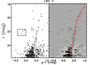
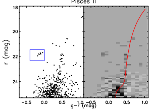
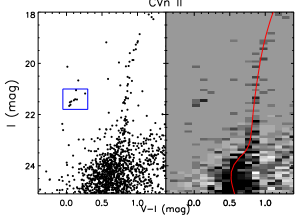
Figure 1.— Color magnitude diagrams of our three satellites – Leo V (Left), Pisces II (Middle), and CVn II (Right) – utilizing data within two half light radii (see § 4.1). Each satellite’s figure is split into two panels. On the left are the raw CMDs. The inset box shows our initial selection region for BHB stars, which we will use as our starting point for studying their spatial distribution in § 4.2. On the right is overplotted a theoretical isochrone from Girardi et al. (2004) with [Fe/H]=$-2.0$ and 13.5 Gyr age.

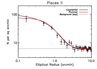
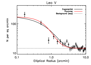
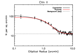
Figure 2.— Stellar profiles of Leo V, Pisces II and CVn II, where the data points are the binned star counts for stars consistent with the CMD ridgeline of each object. The plotted lines show the best-fit one-dimensional exponential and Plummer profiles, found via our ML analysis in § 4.1. The dotted line shows the background surface density determined for our exponential profile fit. Note that in deriving our profile fits, we are not fitting to the binned data, but directly to the two-dimensional stellar distribution.

Figure 3.— Two-dimensional, marginalized confidence contours (corresponding to the 68%, 95% and 99% confidence limits) for the half light radius, ellipticity and position angle for the three dwarfs in our study. These contours are for the exponential profile fit.

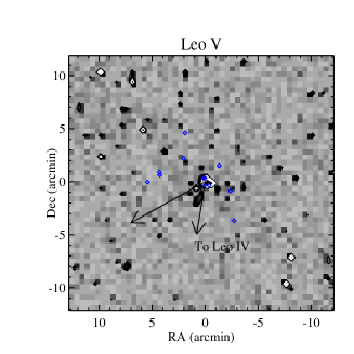
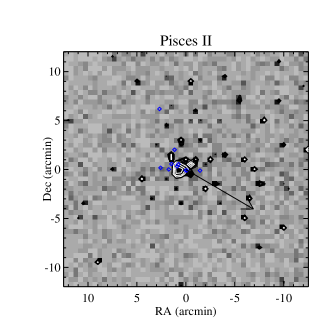
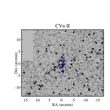
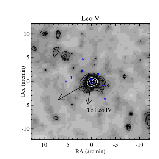
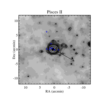
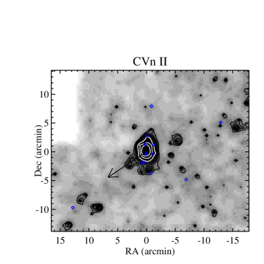
Figure 4.— Top row – Matched filter maps of Leo V, Pisces II and CVn II, with the contour levels showing the 5, 6, 7, 10, 15 and 20 $\sigma$ levels above the modal value in each map. The pixel size in each map is 30 arcseconds, with no smoothing. Each dwarf is clearly visible in the center of each field. Bottom row – Matched filter maps of Leo V, Pisces II and CVn II, with the contour levels showing the 3, 4, 5, 6, 7, 10, 15 and 20 $\sigma$ levels above the modal value in each map (although, since these maps have been smoothed, these $\sigma$ levels cannot be thought of in the traditional sense). The pixel size of each map is 20 arcseconds, and has been smoothed by a Gaussian with width 30 arcseconds. The arrow in each plot points to the Galactic Center. The blue diamonds are likely BHB stars. Note that the second arrow in the Leo V map is pointing in the direction of Leo IV, with no sign of extended structure in its direction. Note the Subaru chip that was left out of our analysis for the CVn II maps, as explained in § 2.

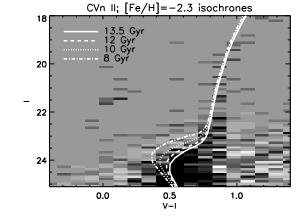
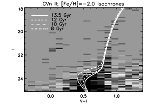
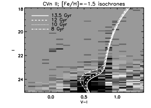
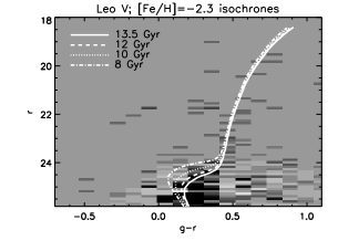
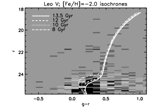
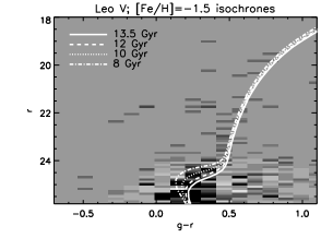
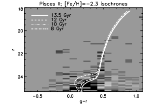
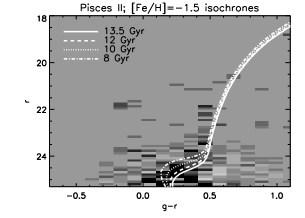
Figure 5.— Hess diagrams of CVnII, Leo V and Pisces II within 2$r_{h}$, with a background CMD subtracted. We have also overplotted theoretical isochrones from Girardi et al. (2004) in order to qualitatively assess the stellar populations which are compatible with the data – see § 5.1 for details.

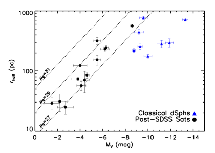
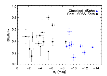
Figure 6.— Distribution of the MW satellites in the $M_{V}$ vs. $r_{half}$ (left) and $M_{V}$ vs. $\epsilon$ (right) planes. Note that CVn I, although discovered in the SDSS, has similar properties as the classical dSphs in both panels. The apparent decline in half-light radius as a function of magnitude among the new MW satellites may be artificial, as objects that are ‘large and faint’ would have gone undetected by the SDSS survey (Walsh et al. 2009; Koposov et al. 2009), but would sit in the upper left corner of the plot. Lines of constant surface brightness are shown to highlight this selection effect. As discussed in § 6.2, there is little statistical evidence that the post-SDSS satellites and the classical dSphs have a different ellipticity distribution, as portrayed in the right panel. However, Hercules ($\epsilon=0.67$) and Ursa Major I ($\epsilon=0.80$) still stand out in this plot.

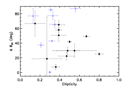
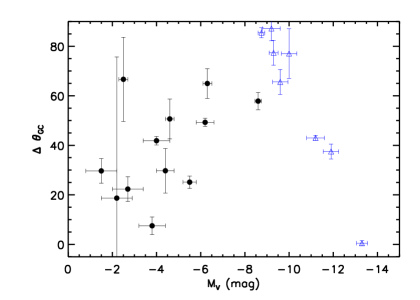
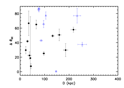
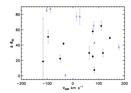
Figure 7.— Here we plot the difference in angle between the major axis of the MW satellites and the direction to the MW center ($\Delta\theta_{GC}$) as a function of various satellite properties. As in Figure 6, the black circles represent the new MW satellites, while the blue triangles are the classical dSphs. In the upper left panel, we plot $\Delta\theta_{GC}$ as a function of satellite ellipticity, $\epsilon$. Note that the new MW satellites with the highest ellipticity ($\epsilon\gtrsim 0.4$) tend to have $20^{\circ}\lesssim\Delta\theta_{GC}\lesssim 40^{\circ}$. In the upper right panel we show $\Delta\theta_{GC}$ as a function of satellite luminosity ($M_{V}$) and note that the faintest of the new MW satellites also are the most aligned with the MW center. One obvious exception is the satellite Segue 2. There is no apparent relation between distance to the MW, $D$, and $\Delta\theta_{GC}$; nor with the satellites’ velocity with respect to the Galactic standard of rest ($V_{GSR}$), as can be seen in the bottom two panels. Note that neither Pisces II or Leo IV are represented in these plots, as their position angle is not well determined.

References

- REV (????) ????
- 08 (1) 08. 1
- Adén et al. (2009) Adén, D., Wilkinson, M. I., Read, J. I., Feltzing, S., Koch, A., Gilmore, G. F., Grebel, E. K., & Lundström, I. 2009, ApJ, 706, L150
- An et al. (2008) An, D., Johnson, J. A., Clem, J. L., Yanny, B., Rockosi, C. M., Morrison, H. L., Harding, P., Gunn, J. E., Allende Prieto, C., Beers, T. C., Cudworth, K. M., Ivans, I. I., Ivezić, Ž., Lee, Y. S., Lupton, R. H., Bizyaev, D., Brewington, H., Malanushenko, E., Malanushenko, V., Oravetz, D., Pan, K., Simmons, A., Snedden, S., Watters, S., & York, D. G. 2008, ApJS, 179, 326
- Bellazzini et al. (2005) Bellazzini, M., Gennari, N., & Ferraro, F. R. 2005, MNRAS, 360, 185
- Bellazzini et al. (2004) Bellazzini, M., Gennari, N., Ferraro, F. R., & Sollima, A. 2004, MNRAS, 354, 708
- Belokurov et al. (2008) Belokurov, V., Walker, M. G., Evans, N. W., Faria, D. C., Gilmore, G., Irwin, M. J., Koposov, S., Mateo, M., Olszewski, E., & Zucker, D. B. 2008, ApJ, 686, L83
- Belokurov et al. (2010) Belokurov, V., Walker, M. G., Evans, N. W., Gilmore, G., Irwin, M. J., Just, D., Koposov, S., Mateo, M., Olszewski, E., Watkins, L., & Wyrzykowski, L. 2010, ApJ, 712, L103
- Belokurov et al. (2009) Belokurov, V., Walker, M. G., Evans, N. W., Gilmore, G., Irwin, M. J., Mateo, M., Mayer, L., Olszewski, E., Bechtold, J., & Pickering, T. 2009, MNRAS, 397, 1748
- Belokurov et al. (2007) Belokurov, V., Zucker, D. B., Evans, N. W., Kleyna, J. T., Koposov, S., Hodgkin, S. T., Irwin, M. J., Gilmore, G., Wilkinson, M. I., Fellhauer, M., Bramich, D. M., Hewett, P. C., Vidrih, S., De Jong, J. T. A., Smith, J. A., Rix, H.-W., Bell, E. F., Wyse, R. F. G., Newberg, H. J., Mayeur, P. A., Yanny, B., Rockosi, C. M., Gnedin, O. Y., Schneider, D. P., Beers, T. C., Barentine, J. C., Brewington, H., Brinkmann, J., Harvanek, M., Kleinman, S. J., Krzesinski, J., Long, D., Nitta, A., & Snedden, S. A. 2007, ApJ, 654, 897
- Belokurov et al. (2006) Belokurov, V., Zucker, D. B., Evans, N. W., Wilkinson, M. I., Irwin, M. J., Hodgkin, S., Bramich, D. M., Irwin, J. M., Gilmore, G., Willman, B., Vidrih, S., Newberg, H. J., Wyse, R. F. G., Fellhauer, M., Hewett, P. C., Cole, N., Bell, E. F., Beers, T. C., Rockosi, C. M., Yanny, B., Grebel, E. K., Schneider, D. P., Lupton, R., Barentine, J. C., Brewington, H., Brinkmann, J., Harvanek, M., Kleinman, S. J., Krzesinski, J., Long, D., Nitta, A., Smith, J. A., & Snedden, S. A. 2006, ApJ, 647, L111
- Bonanos et al. (2004) Bonanos, A. Z., Stanek, K. Z., Szentgyorgyi, A. H., Sasselov, D. D., & Bakos, G. Á. 2004, AJ, 127, 861
- Bovill & Ricotti (2011a) Bovill, M. S. & Ricotti, M. 2011a, ApJ, 741, 17
- Bovill & Ricotti (2011b) —. 2011b, ApJ, 741, 18
- Bullock et al. (2010) Bullock, J. S., Stewart, K. R., Kaplinghat, M., Tollerud, E. J., & Wolf, J. 2010, ApJ, 717, 1043
- Carrera et al. (2002) Carrera, R., Aparicio, A., Martínez-Delgado, D., & Alonso-García, J. 2002, AJ, 123, 3199
- Catelan (2009) Catelan, M. 2009, Ap&SS, 320, 261
- Cho et al. (2005) Cho, D.-H., Lee, S.-G., Jeon, Y.-B., & Sim, K. J. 2005, AJ, 129, 1922
- Coleman et al. (2007) Coleman, M. G., de Jong, J. T. A., Martin, N. F., Rix, H.-W., Sand, D. J., Bell, E. F., Pogge, R. W., Thompson, D. J., Hippelein, H., Giallongo, E., Ragazzoni, R., DiPaola, A., Farinato, J., Smareglia, R., Testa, V., Bechtold, J., Hill, J. M., Garnavich, P. M., & Green, R. F. 2007, ApJ, 668, L43
- Combes et al. (1999) Combes, F., Leon, S., & Meylan, G. 1999, A&A, 352, 149
- Dall’Ora et al. (2006) Dall’Ora, M., Clementini, G., Kinemuchi, K., Ripepi, V., Marconi, M., Di Fabrizio, L., Greco, C., Rodgers, C. T., Kuehn, C., & Smith, H. A. 2006, ApJ, 653, L109
- de Jong et al. (2008a) de Jong, J. T. A., Harris, J., Coleman, M. G., Martin, N. F., Bell, E. F., Rix, H.-W., Hill, J. M., Skillman, E. D., Sand, D. J., Olszewski, E. W., Zaritsky, D., Thompson, D., Giallongo, E., Ragazzoni, R., DiPaola, A., Farinato, J., Testa, V., & Bechtold, J. 2008a, ApJ, 680, 1112
- de Jong et al. (2010) de Jong, J. T. A., Martin, N. F., Rix, H.-W., Smith, K. W., Jin, S., & Macciò, A. V. 2010, ApJ, 710, 1664
- de Jong et al. (2008b) de Jong, J. T. A., Rix, H.-W., Martin, N. F., Zucker, D. B., Dolphin, A. E., Bell, E. F., Belokurov, V., & Evans, N. W. 2008b, AJ, 135, 1361
- Dehnen et al. (2004) Dehnen, W., Odenkirchen, M., Grebel, E. K., & Rix, H.-W. 2004, AJ, 127, 2753
- Diemand et al. (2007) Diemand, J., Kuhlen, M., & Madau, P. 2007, ApJ, 667, 859
- Dolphin (2002) Dolphin, A. E. 2002, MNRAS, 332, 91
- Dolphin et al. (2005) Dolphin, A. E., Weisz, D. R., Skillman, E. D., & Holtzman, J. A. 2005, ArXiv Astrophysics e-prints
- Dotter et al. (2007) Dotter, A., Chaboyer, B., Jevremović, D., Baron, E., Ferguson, J. W., Sarajedini, A., & Anderson, J. 2007, AJ, 134, 376
- Dotter et al. (2008) Dotter, A., Chaboyer, B., Jevremović, D., Kostov, V., Baron, E., & Ferguson, J. W. 2008, ApJS, 178, 89
- Fadely et al. (2011) Fadely, R., Willman, B., Geha, M., Walsh, S., Muñoz, R. R., Jerjen, H., Vargas, L. C., & Da Costa, G. S. 2011, AJ, 142, 88
- Girardi et al. (2004) Girardi, L., Grebel, E. K., Odenkirchen, M., & Chiosi, C. 2004, A&A, 422, 205
- Gnedin & Kravtsov (2006) Gnedin, N. Y. & Kravtsov, A. V. 2006, ApJ, 645, 1054
- Greco et al. (2008) Greco, C., Dall’Ora, M., Clementini, G., Ripepi, V., Di Fabrizio, L., Kinemuchi, K., Marconi, M., Musella, I., Smith, H. A., Rodgers, C. T., Kuehn, C., Beers, T. C., Catelan, M., & Pritzl, B. J. 2008, ApJ, 675, L73
- Harris & Zaritsky (2001) Harris, J. & Zaritsky, D. 2001, ApJS, 136, 25
- Harris & Zaritsky (2004) —. 2004, AJ, 127, 1531
- Harris (1996) Harris, W. E. 1996, AJ, 112, 1487
- Irwin & Hatzidimitriou (1995) Irwin, M. & Hatzidimitriou, D. 1995, MNRAS, 277, 1354
- Irwin et al. (2007) Irwin, M. J., Belokurov, V., Evans, N. W., Ryan-Weber, E. V., de Jong, J. T. A., Koposov, S., Zucker, D. B., Hodgkin, S. T., Gilmore, G., Prema, P., Hebb, L., Begum, A., Fellhauer, M., Hewett, P. C., Kennicutt, Jr., R. C., Wilkinson, M. I., Bramich, D. M., Vidrih, S., Rix, H.-W., Beers, T. C., Barentine, J. C., Brewington, H., Harvanek, M., Krzesinski, J., Long, D., Nitta, A., & Snedden, S. A. 2007, ApJ, 656, L13
- Jordi et al. (2006) Jordi, K., Grebel, E. K., & Ammon, K. 2006, A&A, 460, 339
- Kirby et al. (2011) Kirby, E. N., Lanfranchi, G. A., Simon, J. D., Cohen, J. G., & Guhathakurta, P. 2011, ApJ, 727, 78
- Kirby et al. (2008) Kirby, E. N., Simon, J. D., Geha, M., Guhathakurta, P., & Frebel, A. 2008, ApJ, 685, L43
- Klimentowski et al. (2009) Klimentowski, J., Łokas, E. L., Kazantzidis, S., Mayer, L., Mamon, G. A., & Prada, F. 2009, MNRAS, 400, 2162
- Koch et al. (2009) Koch, A., Wilkinson, M. I., Kleyna, J. T., Irwin, M., Zucker, D. B., Belokurov, V., Gilmore, G. F., Fellhauer, M., & Evans, N. W. 2009, ApJ, 690, 453
- Koposov et al. (2008) Koposov, S., Belokurov, V., Evans, N. W., Hewett, P. C., Irwin, M. J., Gilmore, G., Zucker, D. B., Rix, H.-W., Fellhauer, M., Bell, E. F., & Glushkova, E. V. 2008, ApJ, 686, 279
- Koposov et al. (2007) Koposov, S., de Jong, J. T. A., Belokurov, V., Rix, H.-W., Zucker, D. B., Evans, N. W., Gilmore, G., Irwin, M. J., & Bell, E. F. 2007, ApJ, 669, 337
- Koposov et al. (2011) Koposov, S. E., Gilmore, G., Walker, M. G., Belokurov, V., Wyn Evans, N., Fellhauer, M., Gieren, W., Geisler, D., Monaco, L., Norris, J. E., Okamoto, S., Penarrubia, J., Wilkinson, M., Wyse, R. F. G., & Zucker, D. B. 2011, ArXiv e-prints
- Koposov et al. (2009) Koposov, S. E., Yoo, J., Rix, H.-W., Weinberg, D. H., Macciò, A. V., & Escudé, J. M. 2009, ApJ, 696, 2179
- Kraft & Ivans (2003) Kraft, R. P. & Ivans, I. I. 2003, PASP, 115, 143
- Kravtsov (2010) Kravtsov, A. 2010, Advances in Astronomy, 2010
- Lee et al. (2003) Lee, M. G., Park, H. S., Park, J.-H., Sohn, Y.-J., Oh, S. J., Yuk, I.-S., Rey, S.-C., Lee, S.-G., Lee, Y.-W., Kim, H.-I., Han, W., Park, W.-K., Lee, J. H., Jeon, Y.-B., & Kim, S. C. 2003, AJ, 126, 2840
- Marín-Franch et al. (2009) Marín-Franch, A., Aparicio, A., Piotto, G., Rosenberg, A., Chaboyer, B., Sarajedini, A., Siegel, M., Anderson, J., Bedin, L. R., Dotter, A., Hempel, M., King, I., Majewski, S., Milone, A. P., Paust, N., & Reid, I. N. 2009, ApJ, 694, 1498
- Martin et al. (2008a) Martin, N. F., Coleman, M. G., De Jong, J. T. A., Rix, H., Bell, E. F., Sand, D. J., Hill, J. M., Thompson, D., Burwitz, V., Giallongo, E., Ragazzoni, R., Diolaiti, E., Gasparo, F., Grazian, A., Pedichini, F., & Bechtold, J. 2008a, ApJ, 672, L13
- Martin et al. (2008b) Martin, N. F., de Jong, J. T. A., & Rix, H.-W. 2008b, ApJ, 684, 1075
- Mateo et al. (2008a) Mateo, M., Olszewski, E. W., & Walker, M. G. 2008a, ApJ, 675, 201
- Mateo et al. (2008b) —. 2008b, ApJ, 675, 201
- Mateo (1998) Mateo, M. L. 1998, ARA&A, 36, 435
- McLeod et al. (2006) McLeod, B., Geary, J., Ordway, M., Amato, S., Conroy, M., & Gauron, T. 2006, in Scientific Detectors for Astronomy 2005, ed. J. E. Beletic, J. W. Beletic, & P. Amico, 337
- Miyazaki et al. (2002) Miyazaki, S., Komiyama, Y., Sekiguchi, M., Okamura, S., Doi, M., Furusawa, H., Hamabe, M., Imi, K., Kimura, M., Nakata, F., Okada, N., Ouchi, M., Shimasaku, K., Yagi, M., & Yasuda, N. 2002, PASJ, 54, 833
- Momany et al. (2007) Momany, Y., Held, E. V., Saviane, I., Zaggia, S., Rizzi, L., & Gullieuszik, M. 2007, A&A, 468, 973
- Moore et al. (1999) Moore, B., Ghigna, S., Governato, F., Lake, G., Quinn, T., Stadel, J., & Tozzi, P. 1999, ApJ, 524, L19
- Moretti et al. (2009) Moretti, M. I., Dall’Ora, M., Ripepi, V., Clementini, G., Di Fabrizio, L., Smith, H. A., DeLee, N., Kuehn, C., Catelan, M., Marconi, M., Musella, I., Beers, T. C., & Kinemuchi, K. 2009, ApJ, 699, L125
- Muñoz et al. (2005) Muñoz, R. R., Frinchaboy, P. M., Majewski, S. R., Kuhn, J. R., Chou, M.-Y., Palma, C., Sohn, S. T., Patterson, R. J., & Siegel, M. H. 2005, ApJ, 631, L137
- Muñoz et al. (2010) Muñoz, R. R., Geha, M., & Willman, B. 2010, AJ, 140, 138
- Munoz et al. (2011) Munoz, R. R., Padmanabhan, N., & Geha, M. 2011, ArXiv e-prints
- Okamoto et al. (2008) Okamoto, S., Arimoto, N., Yamada, Y., & Onodera, M. 2008, A&A, 487, 103
- Okamoto et al. (2012) —. 2012, ApJ, 744, 96
- Pietrzyński et al. (2008) Pietrzyński, G., Gieren, W., Szewczyk, O., Walker, A., Rizzi, L., Bresolin, F., Kudritzki, R.-P., Nalewajko, K., Storm, J., Dall’Ora, M., & Ivanov, V. 2008, AJ, 135, 1993
- Pietrzyński et al. (2009) Pietrzyński, G., Górski, M., Gieren, W., Ivanov, V. D., Bresolin, F., & Kudritzki, R.-P. 2009, AJ, 138, 459
- Pryor & Meylan (1993) Pryor, C. & Meylan, G. 1993, in Astronomical Society of the Pacific Conference Series, Vol. 50, Structure and Dynamics of Globular Clusters, ed. S. G. Djorgovski & G. Meylan, 357–+
- Ricotti & Gnedin (2005) Ricotti, M. & Gnedin, N. Y. 2005, ApJ, 629, 259
- Rocha et al. (2011) Rocha, M., Peter, A. H. G., & Bullock, J. S. 2011, ArXiv e-prints
- Rockosi et al. (2002) Rockosi, C. M., Odenkirchen, M., Grebel, E. K., Dehnen, W., Cudworth, K. M., Gunn, J. E., York, D. G., Brinkmann, J., Hennessy, G. S., & Ivezić, Ž. 2002, AJ, 124, 349
- Saha et al. (2010) Saha, A., Olszewski, E. W., Brondel, B., Olsen, K., Knezek, P., Harris, J., Smith, C., Subramaniam, A., Claver, J., Rest, A., Seitzer, P., Cook, K. H., Minniti, D., & Suntzeff, N. B. 2010, AJ, 140, 1719
- Sand et al. (2009) Sand, D. J., Olszewski, E. W., Willman, B., Zaritsky, D., Seth, A., Harris, J., Piatek, S., & Saha, A. 2009, ApJ, 704, 898
- Sand et al. (2010) Sand, D. J., Seth, A., Olszewski, E. W., Willman, B., Zaritsky, D., & Kallivayalil, N. 2010, ApJ, 718, 530
- Schlegel et al. (1998) Schlegel, D. J., Finkbeiner, D. P., & Davis, M. 1998, ApJ, 500, 525
- Simon & Geha (2007) Simon, J. D. & Geha, M. 2007, ApJ, 670, 313
- Simon et al. (2011) Simon, J. D., Geha, M., Minor, Q. E., Martinez, G. D., Kirby, E. N., Bullock, J. S., Kaplinghat, M., Strigari, L. E., Willman, B., Choi, P. I., Tollerud, E. J., & Wolf, J. 2011, ApJ, 733, 46
- Stetson (1994) Stetson, P. B. 1994, PASP, 106, 250
- Stinson et al. (2009) Stinson, G. S., Dalcanton, J. J., Quinn, T., Gogarten, S. M., Kaufmann, T., & Wadsley, J. 2009, MNRAS, 395, 1455
- van den Bergh (1994) van den Bergh, S. 1994, ApJ, 428, 617
- van Dokkum (2001) van Dokkum, P. G. 2001, PASP, 113, 1420
- VandenBerg (2000) VandenBerg, D. A. 2000, ApJS, 129, 315
- Walker et al. (2009a) Walker, M. G., Belokurov, V., Evans, N. W., Irwin, M. J., Mateo, M., Olszewski, E. W., & Gilmore, G. 2009a, ApJ, 694, L144
- Walker et al. (2009b) Walker, M. G., Mateo, M., Olszewski, E. W., Peñarrubia, J., Wyn Evans, N., & Gilmore, G. 2009b, ArXiv e-prints
- Walker et al. (2009c) Walker, M. G., Mateo, M., Olszewski, E. W., Sen, B., & Woodroofe, M. 2009c, AJ, 137, 3109
- Walsh et al. (2007) Walsh, S. M., Jerjen, H., & Willman, B. 2007, ApJ, 662, L83
- Walsh et al. (2009) Walsh, S. M., Willman, B., & Jerjen, H. 2009, AJ, 137, 450
- Walsh et al. (2008) Walsh, S. M., Willman, B., Sand, D., Harris, J., Seth, A., Zaritsky, D., & Jerjen, H. 2008, ApJ, 688, 245
- Willman (2010) Willman, B. 2010, Advances in Astronomy, 2010
- Willman et al. (2005a) Willman, B., Blanton, M. R., West, A. A., Dalcanton, J. J., Hogg, D. W., Schneider, D. P., Wherry, N., Yanny, B., & Brinkmann, J. 2005a, AJ, 129, 2692
- Willman et al. (2005b) Willman, B., Dalcanton, J. J., Martinez-Delgado, D., West, A. A., Blanton, M. R., Hogg, D. W., Barentine, J. C., Brewington, H. J., Harvanek, M., Kleinman, S. J., Krzesinski, J., Long, D., Neilsen, Jr., E. H., Nitta, A., & Snedden, S. A. 2005b, ApJ, 626, L85
- Willman et al. (2011) Willman, B., Geha, M., Strader, J., Strigari, L. E., Simon, J. D., Kirby, E., Ho, N., & Warres, A. 2011, AJ, 142, 128
- Willman et al. (2006) Willman, B., Masjedi, M., Hogg, D. W., Dalcanton, J. J., Martinez-Delgado, D., Blanton, M., West, A. A., Dotter, A., & Chaboyer, B. 2006, ArXiv Astrophysics e-prints
- Wolf et al. (2010) Wolf, J., Martinez, G. D., Bullock, J. S., Kaplinghat, M., Geha, M., Muñoz, R. R., Simon, J. D., & Avedo, F. F. 2010, MNRAS, 406, 1220
- Zaritsky & Harris (2004) Zaritsky, D. & Harris, J. 2004, ApJ, 604, 167
- Zucker et al. (2006a) Zucker, D. B., Belokurov, V., Evans, N. W., Kleyna, J. T., Irwin, M. J., Wilkinson, M. I., Fellhauer, M., Bramich, D. M., Gilmore, G., Newberg, H. J., Yanny, B., Smith, J. A., Hewett, P. C., Bell, E. F., Rix, H.-W., Gnedin, O. Y., Vidrih, S., Wyse, R. F. G., Willman, B., Grebel, E. K., Schneider, D. P., Beers, T. C., Kniazev, A. Y., Barentine, J. C., Brewington, H., Brinkmann, J., Harvanek, M., Kleinman, S. J., Krzesinski, J., Long, D., Nitta, A., & Snedden, S. A. 2006a, ApJ, 650, L41
- Zucker et al. (2006b) Zucker, D. B., Belokurov, V., Evans, N. W., Wilkinson, M. I., Irwin, M. J., Sivarani, T., Hodgkin, S., Bramich, D. M., Irwin, J. M., Gilmore, G., Willman, B., Vidrih, S., Fellhauer, M., Hewett, P. C., Beers, T. C., Bell, E. F., Grebel, E. K., Schneider, D. P., Newberg, H. J., Wyse, R. F. G., Rockosi, C. M., Yanny, B., Lupton, R., Smith, J. A., Barentine, J. C., Brewington, H., Brinkmann, J., Harvanek, M., Kleinman, S. J., Krzesinski, J., Long, D., Nitta, A., & Snedden, S. A. 2006b, ApJ, 643, L103