The Lick AGN Monitoring Project: Recalibrating Single-Epoch Virial Black Hole Mass Estimates

Abstract

We investigate the calibration and uncertainties of black hole mass estimates based on the single-epoch (SE) method, using homogeneous and high-quality multi-epoch spectra obtained by the Lick Active Galactic Nucleus (AGN) Monitoring Project for 9 local Seyfert 1 galaxies with black hole masses $<10^{8}~{}{\rm M}_{\odot}$. By decomposing the spectra into their AGN and stellar components, we study the variability of the single-epoch H$\beta$ line width (full width at half-maximum intensity, FWHM_Hβ; or dispersion, $\sigma_{{\rm H}\beta}$) and of the AGN continuum luminosity at 5100 Å ($L_{\rm 5100}$). From the distribution of the “virial products” ($\propto$ FWHM_Hβ² $L_{\rm 5100}^{0.5}$ or $\sigma_{{\rm H}\beta}$² $L_{\rm 5100}^{0.5}$) measured from SE spectra, we estimate the uncertainty due to the combined variability as $\sim 0.05$ dex (12%). This is subdominant with respect to the total uncertainty in SE mass estimates, which is dominated by uncertainties in the size-luminosity relation and virial coefficient, and is estimated to be $\sim 0.46$ dex (factor of $\sim 3$). By comparing the H$\beta$ line profile of the SE, mean, and root-mean-square (rms) spectra, we find that the H$\beta$ line is broader in the mean (and SE) spectra than in the rms spectra by $\sim 0.1$ dex (25%) for our sample with FWHM_Hβ $<3000$ km s^-1. This result is at variance with larger mass black holes where the difference is typically found to be much less than $0.1$ dex. To correct for this systematic difference of the H$\beta$ line profile, we introduce a line-width dependent virial factor, resulting in a recalibration of SE black hole mass estimators for low-mass AGNs.

1. INTRODUCTION

Supermassive black holes (BHs) are believed to play a key role in galaxy evolution. Evidence for this connection comes from the tight correlations observed in the local universe between BH masses and the global properties of their host galaxies (Magorrian et al. 1998; Ferrarese & Merritt 2000; Gebhardt et al. 2000; Gültekin et al. 2009; Bentz et al. 2009a; Woo et al. 2010). Establishing the cosmic evolution of these correlations is a powerful way to understand the feedback mechanisms connecting BHs and galaxies (e.g., Kauffmann & Haehnelt 2000; Robertson et al. 2006; Hopkins et al. 2006). Recent observational studies have found that these correlations may evolve over cosmic time, in the sense that BHs of a given mass appeared to live in smaller galaxies in the past (e.g., Woo et al. 2006; Peng et al. 2006; Treu et al. 2007; Woo et al. 2008; Merloni et al. 2010; Decarli et al. 2010; Bennert et al. 2010).

In order to investigate the nature of BH-galaxy coevolution, as well as virtually all aspects of active galactic nucleus (AGN) physics (e.g., Woo & Urry 2002; Kollmeier et al. 2006; Davis et al. 2007), BH masses must be accurately determined at large distances. Dynamical methods based on high angular resolution kinematics of stars and gas are the most common approach to measuring masses of quiescent BHs (e.g., Kormendy & Gebhardt 2001; Ferrarese & Ford 2005). However, owing to the parsec-size scale of the sphere of the influence of typical BHs, they are limited to galaxies within a distance of few tens of Mpc with current technology.

In the case of BHs powering an AGN, the presence of a variable broad-line region (BLR) provides an alternative way that is in principle applicable to much larger distances. The geometry and kinematics of the BLR gas can be mapped in the time domain using the so-called reverberation (or echo) mapping technique (Blandford & McKee 1982; Peterson 1993). In turn, these quantities can be converted into BH mass estimates under appropriate assumptions about the dynamics of the system (Peterson 1993; Pancoast, Brewer, & Treu 2011). Estimators of the form $M_{\rm BH}$ $\propto R_{\rm BLR}~{}V^{2}$, where $R_{\rm BLR}$ and $V$ are (respectively) size and velocity estimators of the BLR, are often referred to as “virial” mass estimators. However, due to the observational challenges of reverberation mapping campaigns, fewer than 50 BH masses have been measured to date using this technique (Wandel, Peterson, & Malkan 1999; Kaspi et al. 2000; Peterson et al. 2004; Bentz et al. 2009c; Denney et al 2009; Barth et al. 2011).

In light of the scientific importance of determining BH masses, it is critical to develop alternative BH mass estimators that are observationally less demanding. A popular BH mass estimator, based on the results of reverberation mapping studies, is the so-called single-epoch (SE) method. It exploits the empirical correlation between the size of the BLR and the AGN continuum luminosity ($R_{\rm BLR}\propto L^{\alpha}$, with $\alpha\approx 0.5$), as expected from the photoionization model predictions (Wandel, Peterson, & Malkan 1999; Kaspi et al. 2000, 2005; Bentz et al. 2006, 2009b), to bypass the expense of a monitoring campaign. Thus, the AGN luminosity is used as a proxy for the BLR size and, in combination with the square of a velocity estimate from a broad line, to estimate BH masses from single spectroscopic observations. Typically, SE mass estimators are based on optical/ultraviolet lines (e.g., H$\beta$ or Mg II) and optical/ultraviolet continuum luminosity (e.g., at 5100 Å or 3000 Å). A summary and cross-calibration of commonly adopted recipes is given by McGill et al. (2008).

Due to its convenience, the SE method has been widely applied from the study of BH demographics (e.g., Shen et al. 2008; Fine et al. 2008) to the characterization of galaxy-AGN scaling relations at low and high redshift (e.g., Treu et al. 2004; Barth et al. 2005; Greene & Ho 2006; Woo et al. 2006; Bennert et al. 2010, Bennert et al. 2011a). For this reason it is of paramount importance to quantify, understand, and (possibly) correct for random and systematic uncertainties in the method. In addition to the random and systematic errors, selection bias can play a role in studying statistical properties of AGN samples selected from a flux-limited survey since BH mass from SE data is proportional to the AGN continuum luminosity at 5100Å ($L_{5100}$) (e.g., Lauer et al. 2007; Treu et al. 2007; Shen & Kelly 2010). Naturally, the strength of the selection bias depends on the uncertainty of the SE mass estimates, providing another compelling reason to quantify it accurately.

The largest uncertainty comes from the unknown “virial” factor $f$, connecting the observable size and velocity to the actual BH mass, $M_{\rm BH}$ $\equiv fR_{\rm BLR}~{}V^{2}/G$, where $G$ is the gravitational constant. In general, $f$ cannot be determined for individual sources due to limited spatial information except a few cases (Davies et al. 2006, Onken et al. 2007; Hicks & Malkan 2008; see, however, Brewer et al. 2011 and references therein). Therefore, an average virial factor is typically applied. This average is determined by forcing active and quiescent galaxies to obey the same BH mass-galaxy velocity dispersion ($M_{\rm BH}-\sigma_{*}$) relation (Onken et al. 2004; Woo et al. 2010), even though the virial factor of individual AGNs may be different from the mean value. Thus, using an average virial factor introduces an uncertainty in the SE mass estimates. It is not known precisely how large the uncertainty of the virial factor is (see Collin et al. 2006), and whether this uncertainty is stochastic (random) or has a systematic component that can be reduced using additional observables. An upper limit to the uncertainty is derived from the intrinsic scatter of the AGN $M_{\rm BH}-\sigma_{*}$ relation (0.43 dex; Woo et al. 2010), assuming that the samples used to calibrate $f$ are representative of the class of broad-line AGNs targeted for the SE study.

A second source of uncertainty is the variability of AGNs: line width and continuum luminosity will vary as a function of time, while the BH mass is not expected to change significantly over time scales of order a few years. Thus, AGN variability introduces an uncertainty in the SE mass estimates, which is believed to be stochastic in nature. Previous studies based on multi-epoch spectra reported that the random error due to the variability is $\sim$15–25% (e.g., Woo et al. 2007; Denney et al. 2009).

A third source of error is the intrinsic scatter in the size-luminosity relation used to infer the size of the BLR. Recent studies, based on reverberation mapping results and Hubble Space Telescope (HST) imaging analysis, report $\sim$40% scatter in the size-luminosity relation (Bentz et al. 2009b).

A fourth source of uncertainty in SE mass estimates is due to differences in the BLR line profile as measured from SE spectra and those measured from root-mean-square (rms) spectra. In reverberation mapping studies, BH mass determinations rely on the line width measured from the rms spectra, which reflect the varying part of the line profile. In contrast, for SE mass determinations line widths are measured from single spectra since such equivalent measurements as in the rms spectra are not available. Thus, it is necessary to investigate and quantify the line-width difference between SE and rms spectra. Previous studies based on multi-epoch data showed that the H$\beta$ line widths in the mean spectra are broader than those in the rms spectra (e.g., Sergeev et al. 1999; Shapovalova et al. 2004; Collin et al. 2006; Denney et al. 2009). The difference is presumably due to the different kinematics of the gas responding over various time scales, indicating that a different normalization is required in order to consistently estimate virial masses based on the SE method.

In this work, we focus on the uncertainties of SE mass estimators due to the variability, and those due to differences in line profiles. By comparing measurements from single-epoch, mean, and rms spectra using the high-quality multi-epoch spectra of 9 local Seyfert galaxies in the relatively unexplored regime of low-mass BHs from the Lick AGN monitoring project (Bentz et al. 2009c), we provide new quantitative estimates for the uncertainties and recipes to correct for them. The paper is organized as follows. In §2, we describe the observations and data reduction. Section 3 discusses the measurement method for SE spectra as well as for mean and rms spectra. In § 4, we present the main results including a test of the virial assumption, a quantification of the random errors due to AGN variability, and the systematic differences in line width between SE and rms spectra. We also present a recalibration of standard recipes that corrects for the systematic differences. We conclude and summarize our findings in § 5. Throughout the paper we adopt the following cosmological parameters to calculate distances: $H_{0}=70$ km s^-1 Mpc^-1, $\Omega_{\rm m}=0.30$, and $\Omega_{\Lambda}=0.70$.

2. OBSERVATIONS AND DATA REDUCTION

We use the homogeneous and high-quality multi-epoch spectra from the Lick AGN monitoring project (LAMP; Bentz et al. 2009c), which was designed to measure the reverberation time scales of 13 local Seyfert 1 galaxies. Here, we briefly summarize the observations and data reduction.

The LAMP campaign was carried out using the Kast spectrograph at the 3-m Shane telescope at the Lick Observatory in Spring 2008. Among 13 Seyfert 1 galaxies, we selected 9 objects for which the H$\beta$ line variability was sufficiently large to measure the reverberation time lag (Bentz et al. 2009c). During the LAMP campaign, each object was observed multiple times (43 to 51 epochs with an average of 47), enabling us to construct high-quality mean and r.m.s. spectra.

After performing standard spectroscopic reductions using IRAF, one-dimensional spectra were extracted with an aperture window of 13 pixels (10$\farcs$1). Flux calibrations utilized nightly spectra of spectrophotometric standard stars. As described by Bentz et al. (2009c), the spectral rescaling was performed using the algorithm of van Groningen & Wanders (1992) in order to mitigate the effects of slit loss, variable seeing, and transparency. By rescaling, shifting, and smoothing each spectrum, the algorithm minimizes the difference of flux of the [O III] lines between each spectrum and a reference spectrum created from the mean of individual spectra. The quality of each individual spectrum is sufficient to perform SE measurements (average signal-to-noise ratio S/N $\approx 66$ per pixel at rest-frame 5100 Å).

3. MEASUREMENTS

Two quantities, the line width and the continuum luminosity, are required to determine $M_{\rm BH}$ using single spectra. Uniform and consistent analysis is crucial for investigating systematic uncertainties and minimizing additional errors. In this section, we present the multi-component spectral fitting process and describe the measurements using single-epoch, mean, and rms spectra.

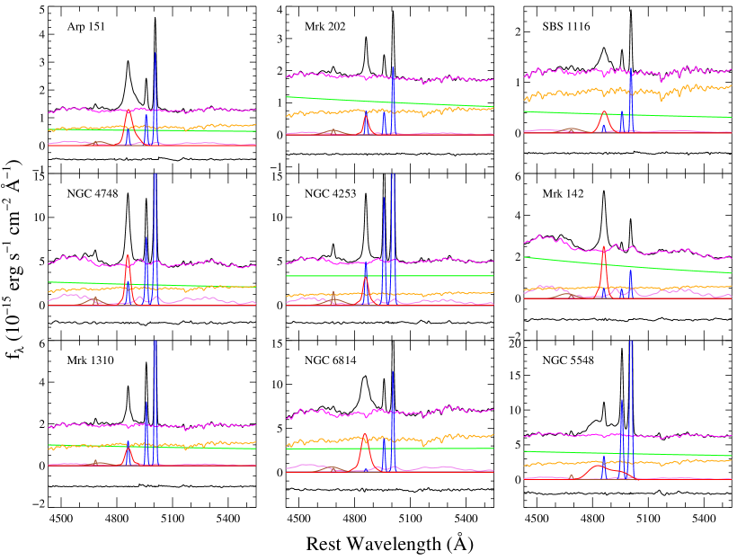
Figure 1.— Multi-component spectral fitting in the mean spectra. The mean spectra of all 9 Seyfert galaxies are presented along with multi-component models. In each panel, observed spectra (black) and the continuum$+$Fe II$+$stellar best-fit model (magenta) are shown in the upper part, and the best-fit power-law continuum (green), stellar spectrum (yellow), and Fe II template (violet) models are presented in the middle part. Three narrow lines [H$\beta$, [O III] $\lambda\lambda 4959,5007$ (blue)], broad H$\beta$ (red), and the broad and narrow He II $\lambda 4686$ components (brown) are presented in the bottom part. The residuals (black), representing the difference between the observed spectra and the sum of all model components, are arbitrarily shifted downward for clarity.

3.1. Multi-Component Fitting

To measure the line width of H$\beta$ and the continuum luminosity at 5100 Å, we follow the procedure given by Woo et al. (2006) and McGill et al. (2008), but with significant modifications as described below (cf., McLure & Dunlop 2004; Dietrich et al. 2005; Denney et al. 2009). The multi-component fitting processes were carried out in a simultaneous and automated fashion, using the nonlinear Levenberg-Marquardt least-squares fitting routine mpfit (Markwardt, 2009) in IDL.

First, all single spectra were converted to the rest frame. Second, we modelled the observed continuum with three components: the featureless AGN continuum, the Fe II emission blends, and the host-galaxy starlight, using respectively a single power-law continuum, an Fe II template from Boroson & Green (1992), and a host-galaxy template from Bruzual & Charlot (2003). A simple stellar population synthesis model with solar metallicity and age of 11 Gyr was found to reproduce the observed stellar lines reasonably well (see Figure 1). The Fe II emission blends and the host-galaxy template were convolved with appropriate Gaussian velocities to reproduce kinetic and instrumental broadening during the fitting process as described below. The best continuum models were determined based on the $\chi^{2}$ statistic in the regions 4430–4600 Å and 5080–5550 Å where Fe II emission dominates. The three components were varied simultaneously with six free parameters: the normalization and the slope of the power-law continuum, the strength and the broadening velocity of the Fe II, and the line strength and the velocity dispersion of the host-galaxy templates. We masked out the typical weak AGN narrow emission lines (e.g., He I $\lambda 4471$, [Fe VII] $\lambda 5160$, [N I] $\lambda 5201$ , [Ca V] $\lambda 5310$; Vanden Berk et al. 2001) during the fitting process. The best-fit continuum models (the power-law component + the Fe II template + the host-galaxy template) were subtracted from each spectrum, leaving the broad and narrow AGN emission lines.

Table 1H$\beta$ Integration Ranges, and H$\beta$ narrow ratios

Object	H$\beta_{\rm BC}$ Line Ranges	$f$(H$\beta_{\rm NC}$)/$f$([O III] $\lambda 5007$)
	(Å)
Arp 151	4790–4980	0.18
NGC 4748	4790–4920	0.12
Mrk 1310	4800–4920	0.13
Mrk 202	4810–4920	0.35
NGC 4253 (Mrk 766)	4790–4930	0.13
NGC 6814	4760–4950	0.03
SBS 1116+583A	4795–4940	0.12
Mrk 142	4790–4910	0.37
NGC 5548	4705–5040	0.10

Note. — All values in the table are given in the rest frame.

Third, we subtracted the narrow lines around the H$\beta$ region before fitting the broad component. We first made a template for the H$\beta$ narrow-line profile by fitting a tenth-order Gauss-Hermite series (cf., van der Marel & Franx 1993) model to the [O III] $\lambda 5007$ line. We then subtracted the [O III] $\lambda 4959$ line by blueshifting and scaling the flux of the template by $1/3$. The H$\beta$ narrow line was also subtracted by scaling the [O III] $\lambda 5007$ line. The ratios of the narrow H$\beta$ to [O III] $\lambda 5007$ were determined from the $\chi^{2}$ minimization in the mean spectra and then forced to be the same for all SE spectra of each object. Applied scaling ratios for the H$\beta$ narrow component range from 0.03 to 0.37 (Table 1).

Lastly, we modelled the broad component of the H$\beta$ line using a sixth-order Gauss-Hermite series. We also used a two-component Gaussian model to describe the broad and narrow components of the He II $\lambda 4686$ emission line whenever it affected the blue wing of the H$\beta$ profile. Figure 1 shows the fitting results for the mean spectra.

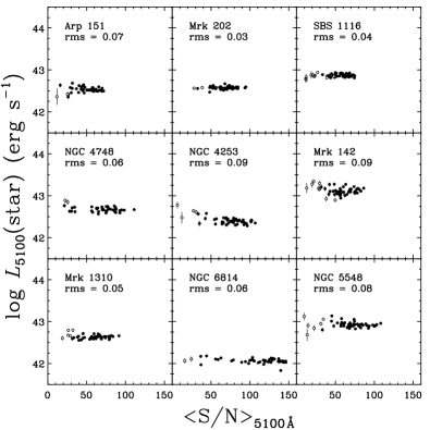
Figure 2.— The host-galaxy luminosity at 5100 Å, measured from each SE spectrum based on the spectral decomposition analysis, as a function of S/N. A few low-S/N spectra (open circles) are removed from further analysis to avoid biases due to low-quality data. Measurement uncertainties estimated from the method given in §3.2.3 are expressed by vertical error bars.

3.2. Single-Epoch Spectra

We performed the multi-component fitting procedure using individual SE spectra, and measured the line width and continuum luminosity for each epoch. The vast majority of SE spectra have sufficiently high quality to perform the analysis (S/N $\approx 66$ per pixel at rest-frame 5100 Å). However, a small fraction of spectra have significantly lower S/N owing to bad weather during the LAMP monitoring campaign. In addition, there are a few epochs with artificial signatures, such as bad pixels, abnormal curvature, or fluctuations in the reduced spectra. Those SE spectra were discarded to avoid possible biases due to much larger measurement errors (see Fig. 2). On average, four bad epochs out of 47 nights were removed for each object, except for SBS 1116, for which 11 epochs were eliminated because of a defect between the H$\beta$ and [O III] $\lambda 4959$ lines due to bad pixels in the detector.

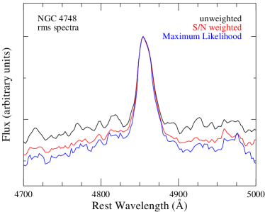
Figure 3.— Comparison of the rms spectra of NGC 4748 generated with three different methods: unweighted rms (black), S/N weighted (red), and maximum likelihood (blue). For this object, two bad epochs with low-S/N data were removed as described in § 3.2.

3.2.1 Emission-Line Width

We measured the full width at half-maximum intensity (FWHM_Hβ) and the dispersion ($\sigma_{{\rm H}\beta}$) (the second moment of line profile; Peterson et al., 2004) of the broad component of H$\beta$ directly from the data as well as from the fits to the continuum-subtracted spectra. Line-width measurements are corrected for the instrumental resolution in a standard way (Barth et al. 2002; Woo et al. 2004; Bentz et al. 2009c), by subtracting in quadrature the instrumental resolution (Table 11 of Bentz et al. 2009c) from the measured line width.

By comparing line widths measured from Gauss-Hermite series fits with those directly measured from the data, we found less than a 3% systematic difference (with considerable rms scatter of $\sim 5$%) as expected given the high S/N of individual spectra. The small systematic trend between FWHM_Hβ and $\sigma_{{\rm H}\beta}$ shows opposite directions. In the case of FWHM_Hβ, the measurements from the fit were $2.6\pm 0.2$% larger than those from the data while $\sigma_{{\rm H}\beta}$ measurements from the fit were $1.9\pm 0.1$% smaller than those from the data, showing a trend consistent with that reported by Denney et al. (2009). For consistency with other studies on the reverberation and single-epoch masses, we focus on the line-width measurements from the fits in the rest of the paper unless explicitly noted.

Table 2Mean continuum luminosities and host-galaxy contributions

Object	$\lambda L_{\lambda}(\mathrm{tot})$	$\lambda L_{\lambda}(\mathrm{AGN})$	$\lambda L_{\lambda}(\mathrm{star})$	$\frac{{\lambda L_{\lambda}(\mathrm{star})}}{{\lambda L_{\lambda}(\mathrm{tot})}}$
	(1042 erg s-1)	(1042 erg s-1)	(1042 erg s-1)
(1)	(2)	(3)	(4)	(5)
Arp 151	$6.11$	$2.76$	$3.42$	$0.56$
NGC 4748	$10.05$	$5.55$	$4.69$	$0.47$
Mrk 1310	$8.10$	$3.79$	$4.32$	$0.53$
Mrk 202	$8.78$	$5.02$	$3.75$	$0.43$
NGC 4253	$8.87$	$6.41$	$2.47$	$0.28$
NGC 6814	$1.93$	$0.83$	$1.15$	$0.59$
SBS 1116+583A	$10.52$	$3.15$	$7.44$	$0.71$
Mrk 142	$47.89$	$35.64$	$12.73$	$0.27$
NGC 5548	$20.86$	$12.42$	$8.37$	$0.40$

Note. — Col. (1): object name. Col. (2): the total continuum luminosity at 5100 Å. Col. (3): the AGN luminosity estimated from the power-law continuum fit. Col. (4): the host-galaxy luminosity estimated from the host-galaxy template fit. Col. (5): the host-galaxy fraction.

3.2.2 Continuum Luminosity

We measured the monochromatic continuum luminosity at 5100 Å from the observed spectra at each epoch by calculating the average flux in the rest-frame 5080–5120 Å region. The luminosity at 5100 Å (total luminosity, $L_{\rm 5100,t}$) is strongly contaminated by the host-galaxy starlight when the AGN luminosity is comparable to or smaller than the host-galaxy stellar luminosity as in the Seyfert galaxies in our sample.

To obtain the AGN continuum luminosity (nuclear luminosity, $L_{\rm 5100,n}$), the host-galaxy contribution to the total luminosity should be subtracted from the measured total luminosity. In principle, the host-galaxy luminosity can be determined by separating a stellar component from a point source using surface brightness fitting analysis based on a high-resolution image. Such an analysis is in progress based on the HST WFC3 images of the LAMP sample (GO-11662, PI. Bentz). For this paper, however, we used the information obtained from the spectral decomposition. We note that, although the host-galaxy flux should be constant, the amount of host-galaxy contribution to the total flux can vary in each epoch’s spectrum because of seeing variations and miscentering in the slit. Thus, the nuclear luminosity, $L_{\rm 5100,n}$, needs to be estimated for each individual spectrum from which Fe II and starlight have been subtracted.

Figure 2 shows the starlight luminosity measured from each SE spectrum as a function of S/N. As expected, the starlight is not constant due to the effects of seeing and miscentering. The variability ranges from 10% to 20% with an average of $0.06\pm 0.01$ dex. These results underscore the importance of subtracting the host-galaxy starlight in making the rms spectra. Otherwise, the rms spectra may contain a contribution from the variable amount of starlight observed through the slit (see § 3.3 and Figure 5).

As a consistency check, we directly compare the host-galaxy flux of NGC 5548 measured from our spectral decomposition with that from the HST imaging analysis as similarly done by Bentz et al. (2009b). In order to calculate the amount of light observed through the spectroscopic aperture, we used an aperture size of $4^{\prime\prime}\times 10\farcs 1$ as used in the LAMP spectroscopy analysis, after smearing the point-spread-function (PSF) subtracted HST image with a $2^{\prime\prime}$ Gaussian seeing disk. The host-galaxy flux of NGC 5548 based on the spectral decomposition is $2.47\times 10^{-15}$ erg s^-1 cm^-2 Å^-1, while the HST imaging-based galaxy flux is $2.73\times 10^{-15}$ erg s^-1 cm^-2 Å^-1. Thus, the small difference ($\sim 10$%) between the two analyses shows the consistency in host-galaxy flux measurements. When we use a smaller seeing disk (e.g., a 1$\farcs$5 Gaussian disk), the host-galaxy flux measured from the HST imaging analysis increases by $\sim 13$%, indicating that the actual seeing size will slightly change the host-galaxy flux measurements.

3.2.3 Error Estimation

To estimate the uncertainties of the line-width and luminosity measurements from SE spectra, we adopted the Monte Carlo flux randomization method (e.g., Bentz et al., 2009c; Shen et al., 2011). First, we generated 50 mock spectra for each observed spectrum by adding Gaussian random noise based on the flux errors at each spectral pixel. Then we measured the line widths and AGN luminosities from the simulated spectra using the method described in §3.2.1 and §3.2.2. We adopted the standard deviation of the distribution of measurements from 50 mock spectra as the measurement uncertainty. For a consistency check, we increased the number of mock spectra up to 100 and found that the results remain the same. In the case of the total luminosity ($L_{\rm 5100,t}$), we measured the uncertainty as the square root of the quadratic sum of the standard deviation of fluxes and average flux errors in the continuum-flux window.

3.3. Mean and RMS Spectra

In this section, we describe the process of generating mean and rms spectra, and present the method for measuring the line width and continuum luminosity. The mean spectra are representative of all single spectra, thus they are useful to constrain the random errors of measurements from single-epoch spectra. In contrast, reverberation mapping studies generally use rms spectra to map the geometry and kinematics of the same gas that responds to the continuum variation. By comparing the line profiles between rms and single spectra, one can investigate any systematic differences of the corresponding line widths, and therefore improve the calibration of BH mass estimators.

3.3.1 Method

We generated mean and rms spectra for each object using the following equations:

$$\left\langle{f(\lambda)}\right\rangle=\frac{1}{N}\sum\limits_{i=1}^{N}{f_{i}(\lambda)},$$ (1)

$${\rm rms}(\lambda)=\sqrt{\frac{1}{{N-1}}\sum\limits_{i=1}^{N}{\left[{f_{i}(\lambda)-\left\langle{f(\lambda)}\right\rangle}\right]^{2}}},$$ (2)

where $f_{i}(\lambda)$ is the flux of $i$-th SE spectrum (out of $N$ spectra).

The unweighted rms spectra can be biased by low-S/N spectra, often showing peaky residual features in the continuum. These spurious features in continuum can affect the wings of the emission lines and therefore the measurement of line dispersion. To mitigate this effect it is best to consider more robust procedures. We considered the following two schemes. First, we used the S/N as a weight, with the following equations:

$$\left\langle{f^{w}(\lambda)}\right\rangle=\sum\limits_{i=1}^{N}{w_{i}f_{i}(\lambda)},$$ (3)

$${\rm rms}^{w}(\lambda)=\sqrt{\frac{1}{{1-\sum\limits_{i=1}^{N}{w_{i}^{2}}}}\sum\limits_{i=1}^{N}{w_{i}\left[{f_{i}(\lambda)-\left\langle{f^{w}(\lambda)}\right\rangle}\right]^{2}}},$$ (4)

where $w_{i}$ is the normalized S/N weight defined by

$$w_{i}=\frac{{\left({S_{i}/N_{i}}\right)}}{{\sum\limits_{i=1}^{N}{\left({S_{i}/N_{i}}\right)}}}.$$ (5)

Alternatively, we considered the maximum likelihood method. Assuming Gaussian errors, the logarithm of the likelihood function (up to a normalization constant) is given by

$$2\ln\mathcal{L}=-\sum\limits_{i=1}^{N}{\ln\epsilon_{{\rm tot},i}^{2}(\lambda)}-\sum\limits_{i=1}^{N}{\frac{{\left[{f_{i}(\lambda)-\left\langle{f(\lambda)}\right\rangle}\right]^{2}}}{{\epsilon_{{\rm tot},i}^{2}(\lambda)}}},$$ (6)

where

$$\epsilon_{{\rm tot},i}^{2}(\lambda)\equiv\epsilon_{i}^{2}(\lambda)+{\rm rms}^{2}(\lambda),$$ (7)

and $\epsilon_{i}(\lambda)$ is the error in the flux $f_{i}(\lambda)$. Here $\left\langle{f(\lambda)}\right\rangle$ is the mean flux while ${\rm rms}(\lambda)$ is the intrinsic scatter – that is, the rms flux after removing measurement errors. By maximizing the log-likelihood, we obtain the mean and rms spectra. The maximum likelihood method also provides proper errors in the rms spectra. We calculated errors in the inferred mean and rms spectra in a standard way, by computing their posterior probability distribution after marginalizing over the other parameters. We adopt $1-\sigma$ errors as symmetric intervals around the posterior peak containing 68.3% of the posterior probability.

Figure 3 compares rms spectra of NGC 4748 generated with the unweighted rms method, the S/N weighted method, and the maximum likelihood method, after removing two bad epochs as described in § 3.2. As expected, the S/N weighted rms spectrum is less noisy than the unweighted rms spectrum. The rms spectrum based on the maximum likelihood method is similar to but slightly noisier than the S/N weighted spectrum. In particular, the maximum likelihood method generates noisy patterns around the [O III] line region, presumably due to the fact that the error statistics have changed owing to the subtraction of the strong [O III] line signals. In the case of the mean spectrum, all three methods produce almost identical results. Thus, we choose the S/N weighting scheme to generate the mean and the rms spectra, and adopt the errors of the rms spectra from the maximum likelihood method. We note that using the rms spectra based on the maximum likelihood method does not significantly change the results in the following analysis. If more bad epochs with low S/N are removed in generating rms spectra (as practiced in the reverberation studies; e.g., Bentz et al. 2009c), the difference among the three methods tends to be smaller.

We note that there may be a potential bias in the S/N weighted method owing to the fact that in the high continuum state the S/N is higher while emission lines are narrower. Thus, the S/N weighted rms spectra can be slightly biased toward having narrower lines. On the other hand, the time lag between the luminosity change and the corresponding velocity change will reduce the bias since the high luminosity and the corresponding narrow line width are not observed at the same epoch.

To test this potential bias, we compared the line-width measurements based on S/N weighted and unweighted rms spectra, respectively. We find that the line width decreases by $2.6\pm 2.1$% for $\sigma_{{\rm H}\beta}$ and $2.7\pm 1.3$% for FWHM_Hβ when the S/N weighted rms spectra are used, indicating that the bias is not significant for our sample AGNs. However, this offset is not due to the luminosity bias since the S/N ratio does not correlate with AGN luminosity. Instead, the change of the S/N ratio is mostly due to the effects of seeing and miscentering within the slit since different amounts of stellar light were observed within the slit on different nights. Considering the low level of luminosity variability and the time lag, the night-to-night seeing and weather variations would be the predominant factors affecting the S/N ratio. The average offset of $\sim$3% is dominated by two objects, NGC 6814 (0.07 dex for $\sigma_{{\rm H}\beta}$, 0.02 dex for FWHM_Hβ) and SBS 1116 (0.04 dex for $\sigma_{{\rm H}\beta}$, 0.05 dex for FWHM_Hβ), which showed the largest stellar fraction in Fig. 1, thus supporting our conclusion. By excluding these two objects, the average offset decreases to $\sim$1%. Thus, we conclude that the potential AGN luminosity bias in the S/N weighted method is not significant, at least for our sample.

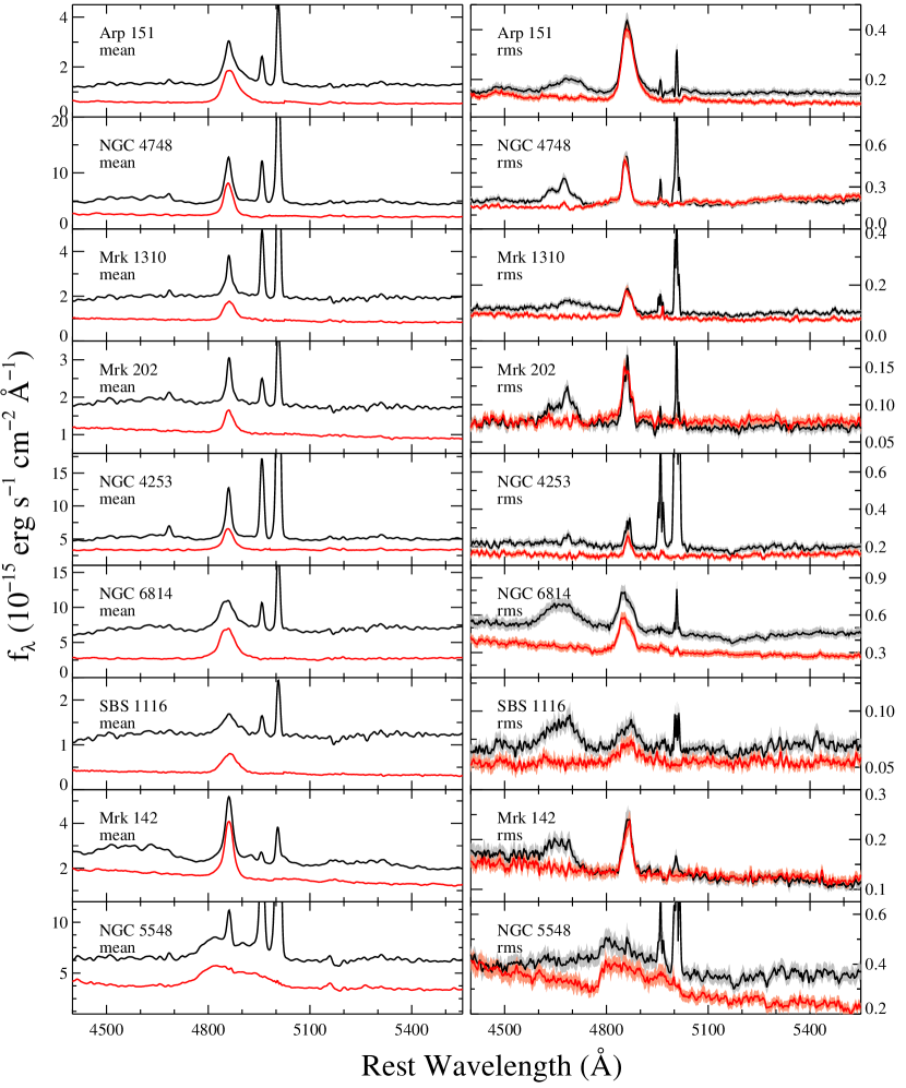
Figure 4.— Left: S/N weighted mean spectra of 9 Seyfert galaxies. Right: S/N weighted rms spectra. In each panel, red lines represent spectra obtained after removing narrow lines, Fe II emission, He II lines, and host-galaxy starlight from each individual SE spectrum. Black lines represent rms spectra obtained without removing the same components from each individual spectrum. Shaded regions show the errors from the maximum likelihood method described in §3.3.

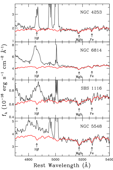
Figure 5.— The rms spectra of 4 Seyfert 1 galaxies with strong stellar features. Black (red) solid lines represent rms spectra (stellar model fit). Strong absorption lines are labelled with arrows.

3.3.2 The Effect of Host Galaxy, Fe II, and He II

Although the rms spectra are supposed to contain only varying components of AGN spectra, residuals of narrow lines (e.g., [O III]) are often present due to residual systematic errors (due to calibration issues; Bentz et al., 2009c). Additionally, the variation of the host-galaxy starlight contribution to the total flux can be significant (10–20%) in the extracted SE spectra as discussed in §3.2.2. This variable starlight is responsible for the stellar absorption features often visible in the rms spectra. To demonstrate the presence of stellar absorption lines in the rms spectra, we fit the continuum with a stellar-population model. As shown in Figure 5, it is clear that the rms spectra show stellar absorption lines [such as the Mg b triplet ($\sim 5175$ Å), Fe (5270 Å), and possibly H$\beta$ (4861 Å)] for Seyfert 1 galaxies having strong starlight contribution. Thus, for AGNs with high starlight fraction, like the ones considered here, it is important to remove the variable starlight in order to generate pure AGN rms spectra and correctly measure the widths of the broad lines.

To minimize these residual features in the rms spectra, we subtracted the narrow lines in all SE spectra before making mean and rms spectra. We also subtracted the Fe II emission blends, host-galaxy starlight, and the He II emission line from each SE spectrum. In Figure 4, we show the S/N weighted mean and rms spectra with and without prior removal of narrow-line components, the Fe II blend, He II lines, and host-galaxy starlight. Clearly, the rms spectra are significantly affected by this procedure. In particular, removing the Fe II and He II emission changes the continuum shape around H$\beta$. For the objects with higher starlight fraction, stellar H$\beta$ absorption is present in the rms spectra, if starlight is not removed from each SE spectrum.

To quantify the change of the line widths due to prior removal of the starlight, He II, and Fe II components, we compared the line-width measurements from rms spectra generated with/without prior removal. Each panel in Fig. 6 shows the effects of individual components by comparing the line-width measurements from the rms spectra with prior removal of all three components (i.e., host-galaxy stellar features, He II, and the Fe II blend) with those from the rms spectra without subtracting one of the three components, respectively. We found that the effect of host-galaxy stellar features is stronger than those of He II and the Fe II blend. Without subtracting host-galaxy stellar features, the rms line widths decrease by $18\pm 5$% for $\sigma_{{\rm H}\beta}$ and $4\pm 3$% for FWHM_Hβ, indicating that the line wings are more affected than the line core. The large increase of $\sigma_{{\rm H}\beta}$ can be understood as the buried H$\beta$ line wings within the residual of stellar features are restored by subtracting the host stellar lines, leading to a lower continuum level and larger line width.

The subtraction of He II changes the line width of objects that show strong blending with the H$\beta$ line (e.g., Mrk 1310 and NGC 6814). On average, the effect of He II on the H$\beta$ line width is at the $4.7\pm 2.2$% level for $\sigma_{{\rm H}\beta}$ and the $1.6\pm 0.6$% level for FWHM_Hβ. In the case of the Fe II subtraction, the effect on the rms line widths is more complex. Line widths increase for some objects and decrease for other objects, depending on whether the Fe II emission residual is strong. For example, if the Fe II residual is prominent in the continuum region (i.e., 5080–5550Å), then the removal of Fe II will lower the continuum level, increasing the H$\beta$ line width. In contrast, if the Fe II residual is strong under H$\beta$, then the H$\beta$ line width will decrease by subtracting Fe II. On average, the effect of Fe II on the H$\beta$  line width is at the $1.2\pm 2.9$% level for $\sigma_{{\rm H}\beta}$ and the $1.6\pm 2.2$% level for FWHM_Hβ.

Without prior removal of all three components (i.e., host-galaxy stellar features, He II, and the Fe II blend), the line widths are underestimated by $18\pm 6$% for $\sigma_{{\rm H}\beta}$  and $5\pm 4$% for FWHM_Hβ, due to the combined effects as described above. Subtracting stellar features has the most significant impact on the measurements of rms line dispersion, demonstrating the importance of prior removal of starlight when stellar contribution is significant. Moreover, in order to successfully remove the He II blending in the rms spectra, the host-galaxy component as well as Fe II emission blends should be simultaneously fitted in the modeling of the continuum. Thus, we conclude that for AGNs with strong host galaxy starlight, strong Fe II, or blended He II, it is necessary to remove all non-broad-line components from SE spectra in order to generate the cleanest rms spectra and reduce errors in measuring the H$\beta$ line width.

3.3.3 Mean Spectra

We generated the S/N weighted mean spectra without prior removal of narrow lines, iron emission, and host-galaxy starlight. Then, we used the same multi-component spectral fitting procedure as used for the SE spectra (see Fig. 1). Note that in the case of mean spectra, removing the narrow lines, Fe II blends, and host-galaxy absorption features before or after generating the mean spectra results in almost identical H$\beta$ broad-line profiles.

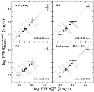
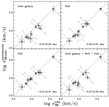
Figure 6.— The effect of each blended component on the rms line widths using the FWHM_Hβ (top) and $\sigma_{{\rm H}\beta}$ (bottom). In each panel, the rms line widths without prior removal of each component (given in the upper-left corner) are plotted as a function of final rms line widths (all non-broad-line components removed). The dashed line indicates an identity relationship. The average offsets with their standard errors are given in the lower-right corner of each panel.

3.3.4 Error Estimation

Using the S/N weighted rms and mean spectra, we measured the widths of the H$\beta$ line from the continuum-subtracted spectra and determined the continuum luminosity at 5100 Å, as described in §3.2.1 and §3.2.2. We estimated the uncertainty of the line-width measurements in the S/N weighted mean and rms spectra using the bootstrap method (e.g., Peterson et al., 2004). One thousand samples per object were generated. The median and standard deviation of the distribution of measurements were adopted as our line-width estimate and uncertainty; these are listed in Table 3. We also estimated the line-width uncertainties for the rms spectra using the method given in §3.2.3. We found that the errors estimated from both the Monte Carlo flux randomization and the bootstrapping were consistent within a few percent on average, which yielded almost identical fitting results.

Table 3Rest-Frame Broad H$\beta$ Line-Width Measurements

Object	Mean Spectrum		RMS Spectrum
	$\sigma_{{\rm H}\beta}$	FWHMHβ	$\sigma_{{\rm H}\beta}$	FWHMHβ
	(km s-1)	(km s-1)	(km s-1)	(km s-1)
Arp 151	$1726\pm 17$	$3076\pm 39$	$1295\pm 37$	$2458\pm 82$
NGC 4748	$952\pm 6$	$1796\pm 8$	$791\pm 80$	$1373\pm 86$
Mrk 1310	$1229\pm 12$	$2425\pm 19$	$921\pm 135$	$1823\pm 157$
Mrk 202	$1047\pm 8$	$1787\pm 15$	$962\pm 67$	$1794\pm 181$
NGC 4253	$1232\pm 9$	$1946\pm 10$	$538\pm 92$	$986\pm 251$
NGC 6814	$1744\pm 12$	$3129\pm 14$	$1697\pm 224$	$2945\pm 283$
SBS 1116+583A	$1460\pm 23$	$3135\pm 36$	$1550\pm 310$	$3202\pm 1127$
Mrk 142	$970\pm 5$	$1671\pm 6$	$700\pm 54$	$1601\pm 224$
NGC 5548	$4354\pm 25$	$12402\pm 111$	$3900\pm 266$	$12539\pm 1927$

4. ANALYSIS AND RESULTS

4.1. Testing the Assumptions of SE BH Mass Estimators

Single-epoch $M_{\rm BH}$ estimates are based on the “virial” assumption and on the empirical relation between BLR size and AGN luminosity. Since $M_{\rm BH}$ does not vary over the time scale of our campaign, AGN luminosity and line velocity should obey the relation $V^{2}\propto L^{-0.5}$. In this section, we test this assumption by studying the relation between the line width and continuum luminosity from individual SE spectra of Arp 151, the object with the highest variability during the LAMP campaign.

In Figure 7 we present the time variation of the line width and luminosity of Arp 151. Line width and luminosity are inversely correlated, although the variability amplitude is smaller in luminosity than in line width. Ideally, the luminosity variability should be four times as large as the line-width variability ($0.042\pm 0.001$ dex and $0.027\pm 0.003$ dex, respectively, for FWHM_Hβ and $\sigma_{{\rm H}\beta}$). However, one must take into account the residual contamination from nonvariable sources to the observed continuum. In fact, the amplitude of the luminosity variability is significantly smaller than expected based on the line-width variability if the total luminosity is used (bottom panel). In contrast, providing a validation of our constant continuum subtraction procedure, the variability amplitude of the nuclear continuum is consistent with that expected from the line width, as we will further quantify below.

In Figure 8, we compare measured luminosities and line widths in order to test whether they obey the expected relation $V^{2}\propto L^{-0.5}$. The continuum variation is shifted by the measured time lag, 4 days, to account for the time delay between the central engine and BLR variations and then matched with the corresponding epochs of line-width variations. Note that densely sampled light curves are required for this correction. As expected, the observed correlation between total flux $L_{\rm 5100,t}$ and line width is steeper than the theoretical correlation. In contrast, the correlation between nuclear flux and line width is consistent with the theoretical expectation. The best-fit slopes are $-1.46\pm 0.31$ (with intrinsic scatter $0.05\pm 0.01$ dex) for FWHM_Hβ, and $-1.09\pm 0.15$ (with intrinsic scatter $0.02\pm 0.01$ dex) for $\sigma_{{\rm H}\beta}$, which is consistent with the expected value of $-1$. The linear correlation coefficients between the nuclear luminosity and the line widths are $-0.86$ for the line dispersion and $-0.77$ for the FWHM, indicating the tighter inverse correlation of continuum luminosity with the line dispersion than with the FWHM.

The agreement of the observed correlations with those expected for an ideal system is remarkable, considering the many sources of noise in the observed velocity-luminosity relation. They include residual errors in the subtraction of the host-galaxy starlight contribution and the measurement uncertainties of line widths and luminosities. The inverse correlation between line width and luminosity further corroborates the use of SE mass estimates (Peterson & Wandel, 1999, 2000; Kollatschny, 2003; Peterson et al., 2004).

Figure 7.— Time variations of the H$\beta$ line width (top: FWHM_Hβ; upper middle: $\sigma_{{\rm H}\beta}$) and the continuum luminosity at 5100 Å (lower middle: nuclear; bottom: total) of Arp 151. The dashed lines represent the average values over the monitoring period. The rms dispersion values are given in each panel.

Figure 8.— Test of SE mass estimates for Arp 151. Each filled circle represents SE measurements after shifting luminosity measurements by the average lag of 4 days (left: total luminosity; right: nuclear luminosity). Dashed lines represent the correlation $L^{0.5}\propto V^{-2}$ expected from the virial theorem and the size-luminosity relation, while solid lines are the best-fit slopes. The values of best-fit slopes and its uncertainties are given in each panel.

4.2. Uncertainties Due to Variability

Since the line width and continuum luminosity of an AGN vary as a function of time, mass estimates from SE spectra may also vary. Owing to its stochastic nature, this variability can be considered a source of random error in SE mass estimates. In this section, we quantify this effect by comparing SE measurements with measurements from the mean spectra.

4.2.1 The Effect of Line-Width Variability

Figure 9.— Distribution of the FWHM_Hβ measured from all SE spectra. Each FWHM_Hβ value is normalized to the FWHM_Hβ measured from the mean spectra. The average rms dispersion of $9$ objects is $0.021\pm 0.004$ dex.

Figure 10.— Same as in Fig. 9, but for $\sigma_{{\rm H}\beta}$. The average rms dispersion of $9$ objects is $0.023\pm 0.003$ dex.

We quantify the dispersion of the distribution of line-width measurements using all SE spectra. This dispersion can be interpreted as a random error due to the combined effect of variability and measurement errors. In Figure 9, we present the distributions of FWHM_Hβ measurements from all SE spectra, after normalizing them by the measurement from the mean spectra. All SE values are normalized to the FWHM measured from the mean spectra. The standard deviation of the FWHM distributions ranges from $0.009$ dex to $0.042$ dex, with an average of $0.021\pm 0.004$ dex ($\sim$5%) across all objects. Note that the standard deviation includes the variability and the measurement error.

In Figure 10, we plot the distributions of line dispersion for all objects. The dispersion of distributions ranges from $0.013$ dex to $0.040$ dex, with an average and rms of $0.023\pm 0.003$ dex ($\sim$5%) for the entire sample. SBS 1116 shows the broadest distribution; however, part of this scatter can be attributed to the residual systematic in the left wing of H$\beta$ due to the bad pixels in the original spectra, as discussed previously.

By averaging the standard deviation of the distribution of the line-width measurements for all 9 objects in the sample, we find that the uncertainty of SE BH mass estimates due to the line-width variation and measurement errors is on average $0.044$ dex. Note that the dispersion of the line-width distribution strongly depends on the variability. For example, Arp 151 has the largest variability amplitude and also the largest variability in the line width. This is expected if line flux correlates with BLR size and both are connected to the BH mass. Based on these results, we conclude that the typical uncertainty of SE mass estimates due to line-width variability is $\sim$10%. However, as discussed below, this uncertainty is partly cancelled out in the virial product by the inverse correlation with the variability of the continuum.

4.2.2 The Effect of Luminosity Variability

Figure 11.— Distribution of nuclear luminosities measured from single-epoch spectra (see §3.2.2). Each luminosity value is normalized to the nuclear luminosity measured from the mean spectra. The standard deviation of the distribution is given in each panel. The average standard deviation of all $9$ objects is $0.048\pm 0.008$ dex.

We now consider the effect of luminosity variability on SE mass estimates. In Figure 11, we present the distributions of the nuclear luminosities at 5100 Å, after normalizing them by the nuclear luminosity measured from the mean spectra. The standard deviation of the luminosity distributions ranges from $0.019$ to $0.097$ dex, with an average of $0.048\pm 0.008$ dex ($\sim$12%), which can be treated as a random error of the continuum luminosity measured from a SE spectrum due to the luminosity variability and measurement error.

Based on the empirical size-luminosity relation, the random errors of the luminosity enter the uncertainty of the SE mass estimates as the square root (i.e., $0.024$ dex). This is somewhat smaller than the uncertainty of SE mass estimates due to the line-width variability, $0.044$ dex, as determined in the previous section, indicating that the two do not cancel each other exactly.

4.2.3 Combined Effect

Since the luminosity and the line width are inversely correlated as $V^{2}\propto L^{-0.5}$, one may expect that the variability of luminosity and line width cancel out in the SE mass estimates. However, the two effects may not compensate each other exactly, for a variety of reasons. First, there is a time lag between continuum and emission-line variability. Second, variations such as in the ionizing flux may indicate that the luminosity at 5100 Å traces the broad-line size only approximately. In order to quantify the combined effect of the continuum luminosity and line-width variability, we thus investigate the distribution of the virial product $L_{5100\AA,n}^{0.5}\times\sigma_{{\rm H}\beta}^{2}$ as measured from SE spectra.

In Figure 12, we present the distribution of the SE virial products, normalized by the virial product measured from the mean spectra. The standard deviation of the distributions can be treated as a random error due to the combined variability and measurement errors. The average rms scatter (corresponding to a source of random measurement errors when using the SE estimator) of the virial products is $0.052\pm 0.006$ dex when the line dispersion ($\sigma_{H\beta}$) is used, and $0.049\pm 0.006$ dex when FWHM_Hβ is used.

In agreement with previous studies (Wilhite et al., 2007; Woo et al., 2007; Denney et al., 2009), these results suggest that BH masses based on SE spectra taken at different epochs are consistent within $\sim 0.05$ dex ($\sim 12$%) uncertainty, negligible with respect to other sources of uncertainty which are believed to add up to $\sim$0.4–0.5 dex (see §5.1).

Figure 12.— Distribution of the SE virial product ($V^{2}\times L^{0.5}$) normalized to that of the mean spectra. H$\beta$ line dispersion is used for the velocity and the nuclear luminosity at 5100 Å, corrected for the host galaxy, is used for the luminosity. The average rms dispersion of all $9$ objects is $0.052\pm 0.006$ dex.

4.3. Systematic Difference between SE and Reverberation Masses

In order to assess the accuracy of the SE mass estimates, we need to compare the SE masses with the masses determined from reverberation mapping. Setting aside potential differences in the virial coefficient, there are two main sources of systematic uncertainties in SE mass estimates. One is the potential difference of the line profile between SE spectra and the rms spectra. The other is the systematic uncertainty of the size-luminosity relation. We postpone discussion of the latter to a future paper when more accurate HST-based nuclear luminosities will be available. Therefore, in this section we focus on the systematic difference of the H$\beta$ line profile and derive new SE mass estimators recalibrated to account for the difference found.

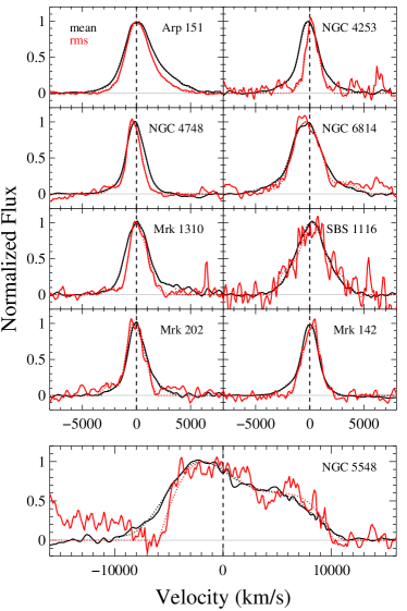
Figure 13.— Comparison of the H$\beta$ broad-line profiles in the mean (black) and rms (red) spectra. In each panel, solid lines represent the data, while dotted lines represent the Gauss-Hermite series fitting results. Each line profile is normalized by the maximum value of the fit. Dashed vertical lines indicate the center of the H$\beta$ line.

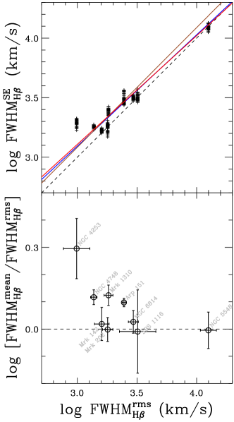
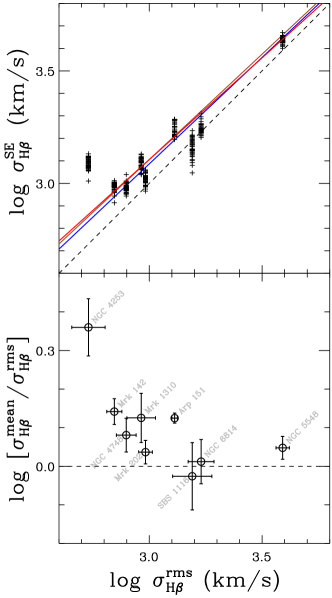
Figure 14.— Direct comparisons of line widths and their ratios, i.e., FWHM_Hβ (left) and $\sigma_{{\rm H}\beta}$ (right), measured from SE (or mean) and rms spectra, as a function of line width. Average offset is $0.07\pm 0.03$ dex for FWHM_Hβ and $0.10\pm 0.04$ dex for $\sigma_{{\rm H}\beta}$. Dashed lines indicate an identity relation while solid lines are the best-fit results using all objects (red), excluding NGC 4253 (blue), or excluding NGC 5548 (brown) using bootstrap errors.

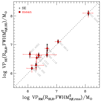
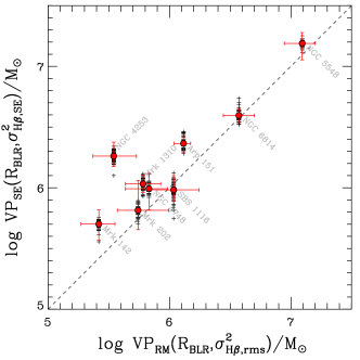
Figure 15.— Comparison of the virial products measured from SE spectra and rms spectra. Virial products are calculated using FWHM_Hβ (top) or $\sigma_{{\rm H}\beta}$ (bottom). In addition to measurements from each SE spectrum (crosses), we show those from the mean spectra (filled circles). The average offset of all mean measurements is $0.201\pm 0.075$ ($0.147\pm 0.066$) dex when $\sigma_{{\rm H}\beta}$ (FWHM_Hβ) is used for the virial products.

4.3.1 Comparing Line Profiles

In Figure 13 we compare the broad H$\beta$ line profiles measured from the mean and rms spectra after normalizing by the peak flux. Generally the H$\beta$ line is broader in the mean spectra than in the rms spectra, indicating that the variation is weaker in the line wings than in the line core. It is worth noting that the observed offset cannot be explained by the contamination of the narrow H$\beta$ component or the Fe II blends since we consistently subtracted them in both the mean and rms spectra. To verify this we arbitrarily decreased the amount of narrow component subtracted from the observed H$\beta$ profile, and found that the large offsets between rms and mean spectra are virtually unchanged.

The broader line width in the mean spectra has been noted in previous reverberation studies (e.g., Sergeev et al. 1999; Shapovalova et al. 2004). Collin et al. (2006) reported that the line widths in the mean spectra were typically broader by $\sim 20$% than those in the rms spectra. Denney et al. (2010) also found that some objects in their reverberation sample clearly showed narrower line widths in the rms spectra than in the mean spectra. Several different and somewhat mutually exclusive explanations have been suggested for this difference. For example, Shields et al. (1995) explained the systematic difference of the line width as being due to the high-velocity gas in the inner BLR being optically thin to the ionizing continuum and hence fully ionized. In this way, the line wings have weak variability and are suppressed in the rms spectra. In contrast, Korista & Goad (2004) suggested a distance-dependent responsivity of optically thick clouds to explain the weak variability of Balmer line wings.

We quantify the systematic offset in line width in Figure 14 by showing the ratios of the line width measured from the mean (and SE) spectra to those measured from the rms spectra as a function of line width. The average offset in FWHM_Hβ is $0.07\pm 0.03$ dex ($0.05\pm 0.02$ dex, if NGC 4253, the object with the narrowest line, is excluded). In the case of line dispersion ($\sigma_{{\rm H}\beta}$), the offset is slightly larger, $0.10\pm 0.04$ dex ($0.07\pm 0.02$ dex if NGC 4253 is excluded). The larger offset of the line dispersion in comparison with FWHM is consistent with there being mainly a difference between variability in the wings and in the core.

There seems to be a systematic trend, in the sense that the offset becomes relatively larger for the narrower line objects, but its origin is not clear. In particular, the narrow-line Seyfert 1 galaxy NGC 4253 (Mrk 766) has the narrowest H$\beta$ line in the sample and shows the largest systematic difference. It is possible that the systematic difference for this particular object with very narrow H$\beta$ (FWHM_Hβ (rms) $<1000$ km s^-1) may be amplified due to imperfect subtraction of the narrow component, the Fe II blends, or starlight. However, the trend is present even if we remove this object from the sample.

In order to correct for this potential bias, we derive a relation between H$\beta$ line width as measured from rms and SE spectra by fitting the trend as shown in Figure 14. Using the linear regression routine linmix_err (Kelly, 2007), we fit the linear relationship in log-scale using bootstrap errors determined in §3.3. We also determined the slope excluding the narrowest-line object (NGC 4253) or the broadest-line object (NGC 5548) from the sample. As shown in Figure 13, removing either NGC 4253 or NGC 5548 from the sample does not significantly change the slope.

In addition, we fit the slope using a fixed error for all objects. Since the bootstrap errors on the rms line widths are significantly different for each object owing to the different quality and S/N ratios of individual single-epoch spectra, we assigned a fixed error, such as 20% on both axes, to test the effect of errors. The best-fit slope using a fixed error is slightly shallower than that with bootstrap errors since the most offset object, NGC 4253 has a large bootstrap error and consequently has smaller weight in the fitting process.

To secure a large dynamic range, we decided to use all 9 objects for the fit and adopt the best-fit result using bootstrap errors. The adopted best fits are expressed as

$$\begin{split}&\log{\rm FWHM}_{\rm H\beta}({\rm rms})=\\ &-0.405(\pm 0.051)+1.095(\pm 0.015)~{}\log{\rm FWHM}_{\rm H\beta}({\rm SE}),\end{split}$$ (8)

$$\log\sigma_{\rm H\beta}(rms)=-0.434(\pm 0.060)+1.106(\pm 0.019)~{}\log\sigma_{\rm H\beta}(SE).$$ (9)

However, these fits should not be extrapolated to high-velocity objects; otherwise, negative bias will be introduced. Since our sample consists of relatively narrow-line Seyfert 1 galaxies, we recommend that readers use Eqs. 8 and 9 for objects with FWHM${}_{\rm H\beta,SE}<3,000$ km s^-1 and $\sigma_{\rm H\beta,SE}<2,000$ km s^-1, respectively.

4.3.2 Systematic Offset of Mass Estimates

The systematically broader line width in SE spectra would result in overestimates of SE masses if unaccounted for. In Figure 15 we plot the ratio of the SE virial product (VP) with respect to the virial product based on the reverberation studies as a function of the virial product. Note that to demonstrate the effect of the systematic difference between SE and rms spectra, we simply used the measured $R_{\rm BLR}$ for all SE virial products, instead of using $L_{5100}$ and the size-luminosity relation. As expected, virial products exhibit a biased systematic trend. The average offset of all SE measurements is $0.152\pm 0.009$ dex when FWHM is used in the virial product (top), and $0.204\pm 0.011$ dex for the $\sigma_{{\rm H}\beta}$-based virial product (bottom). The average offset of all measurements based on mean spectra is $0.147\pm 0.066$ ($0.201\pm 0.075$) dex when FWHM_Hβ ($\sigma_{{\rm H}\beta}$) is used in the virial product. To avoid potential biases from the narrowest-line object, we recalculate the average offset after removing NGC 4253. The average offset of all SE measurements is now $0.093\pm 0.006$ dex and $0.135\pm 0.007$ dex for FWHM_Hβ and $\sigma_{{\rm H}\beta}$, respectively. When the measurements from mean spectra are used in comparison, the average offsets are $0.092\pm 0.040$ dex and $0.136\pm 0.043$ dex for FWHM_Hβ and $\sigma_{{\rm H}\beta}$, respectively. Thus, the SE BH masses of broad-line AGNs with virial products in the range $\sim$10^5-7 M_⊙ can be overestimated by $\sim$25–35% if the same recipe used for rms spectra is adopted.

These results are similar to the findings by Collin et al. (2006), who investigated the systematic offset of virial product estimates between rms and mean spectra using a different sample of reverberation mapping measurements. Although it is not straightforward to directly compare their results with ours since the methods of generating rms spectra and measuring line widths are substantially different, the similar systematic offset between SE and reverberation masses clearly demonstrates the importance of calibrating SE masses.

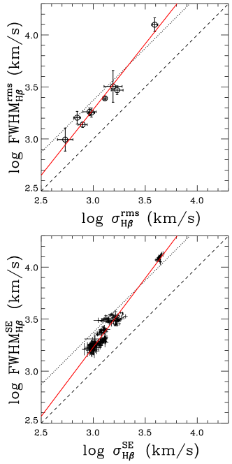
Figure 16.— Comparisons of FWHM_Hβ and $\sigma_{{\rm H}\beta}$, using measurements from rms spectra (top) and SE spectra (bottom). The dashed line indicates an identity relationship while the dotted line represents the Gaussian profile, i.e., FWHM_Hβ/$\sigma_{{\rm H}\beta}$ $=2.35$. The red solid line shows the best-fit relation.

4.3.3 Comparing FWHM_Hβ  and $\sigma_{{\rm H}\beta}$

We compare FWHM_Hβ and $\sigma_{{\rm H}\beta}$ in Figure 15. As previously noticed in other studies (e.g., Collin et al. 2006; McGill et al. 2008), the shape of the H$\beta$ line is different from a Gaussian profile, for which FWHM_Hβ/$\sigma_{{\rm H}\beta}$ is expected to be 2.35. As shown in Figure 16, narrower lines tend to have stronger wings leading to a lower FWHM_Hβ/$\sigma_{{\rm H}\beta}$ ratio, while broader lines are more core dominated with a higher FWHM_Hβ/$\sigma_{{\rm H}\beta}$ ratio. These results are consistent with those of previous studies, although our sample is composed of objects with narrower lines than previously studied.

The best-fit correlation based on the rms spectra is

$$\log{\rm\sigma_{\rm H\beta}}({\rm rms})=0.401(\pm 0.395)+0.792(\pm 0.117)~{}\log{\rm FWHM_{\rm H\beta}}({\rm rms}).$$ (10)

In the case of measurements from the SE spectra, the best fit is expressed as

$$\log{\rm\sigma_{\rm H\beta}}({\rm SE})=0.567(\pm 0.027)+0.753(\pm 0.008)~{}\log{\rm FWHM_{\rm H\beta}}({\rm SE}).$$ (11)

We note that these results are somewhat limited by the small dynamic range of our sample and the lack of objects with FWHM $>3000$ km s^-1. Further analysis with broader line objects is required. However, in the case of broader line objects in the literature, we do not have consistently measured line widths from rms spectra as described in §3.3. Nevertheless, we will use this fit to convert FWHM_Hβ to $\sigma_{{\rm H}\beta}$ in §4.3.4.

4.3.4 Line-Width Dependent Mass Estimators

In order to avoid potential systematic biases in SE spectra, we derive line-width dependent mass estimators, using the best-fit relations derived above (see Fig. 14). As a reference, we use the mass estimator normalized for the virial product from rms spectra (reverberation results) using the virial factor $\log~{}f=0.72$ determined from the $M_{\rm BH}-\sigma_{*}$ relation of reverberation mapped AGNs (Woo et al. 2010):

$$M_{\rm BH}=10^{7.602}{\rm M}_{\odot}\left({\sigma_{{\rm H}\beta}({\rm rms})\over 1000~{}{\rm km~{}s}^{-1}}\right)^{2}\left({\lambda L_{5100,n}\over 10^{44}~{}{\rm erg~{}s}^{-1}}\right)^{0.518}~{}.$$ (12)

If we replace $\sigma_{{\rm H}\beta}$ from rms spectra with $\sigma_{{\rm H}\beta}$ measured from SE spectra using Eq. 9, the mass estimator changes to

$$M_{\rm BH}=10^{7.370}{\rm M}_{\odot}\left({\sigma_{{\rm H}\beta}({\rm SE})\over 1000~{}{\rm km~{}s}^{-1}}\right)^{2.212}\left({\lambda L_{5100,n}\over 10^{44}~{}{\rm erg~{}s}^{-1}}\right)^{0.518}~{}.$$ (13)

As in the case of Eq. 9, we recommend readers use Eq. 13 for AGNs with $\sigma_{{\rm H}\beta}$¡ 2,000 km s^-1.

In the case of FWHM_Hβ, the virial factor has not been determined by Woo et al. (2010), but we can use the relations found above to derive a consistent expression. If we replace $\sigma_{{\rm H}\beta}$ with FWHM_Hβ using Eq. 10, then Eq. 12 becomes

$$M_{\rm BH}=10^{7.156}{\rm M}_{\odot}\left({{\rm FWHM}_{{\rm H}\beta}({\rm rms})\over 1000~{}{\rm km~{}s}^{-1}}\right)^{1.584}\left({\lambda L_{5100,n}\over 10^{44}~{}{\rm erg~{}s}^{-1}}\right)^{0.518}~{}.$$ (14)

In order to use FWHM_Hβ measured from SE spectra, FWHM_Hβ from rms spectra in Eq. 14 can be replaced by FWHM_Hβ from SE spectra, using Eq. 8. Then, the mass estimator becomes

$$M_{\rm BH}=10^{6.966}{\rm M}_{\odot}\left({{\rm FWHM}_{{\rm H}\beta}({\rm SE})\over 1000~{}{\rm km~{}s}^{-1}}\right)^{1.734}\left({\lambda L_{5100,n}\over 10^{44}~{}{\rm erg~{}s}^{-1}}\right)^{0.518}~{}.$$ (15)

Alternatively, we can use Eq. 13 and replace $\sigma_{{\rm H}\beta}$ with FWHM_Hβ measured from SE spectra using Eq. 11. Then Eq. 13 becomes

$$M_{\rm BH}=10^{6.985}{\rm M}_{\odot}\left({{\rm FWHM}_{{\rm H}\beta}(SE)\over 1000~{}{\rm km~{}s}^{-1}}\right)^{1.666}\left({\lambda L_{5100,n}\over 10^{44}~{}{\rm erg~{}s}^{-1}}\right)^{0.518}~{},$$ (16)

which is almost identical to Eq. 15. For a consistency check, we compared the SE masses estimated from Eq. 15 with those from Eq. 16. They are consistent within $\sim$1%, indicating that Eq. 15 and 16 are essentially equivalent. As in the case of Eq. 8, for AGNs with FWHM_Hβ¡ 3,000 km s^-1  we recommend readers use Eq. 16 instead of Eq. 15, since the SE masses derived from Eq. 16 are slightly more consistent with the masses determined from Eqs. 12 and 14.

The BH masses derived from the new mass estimators are consistent with each other within a $\sim$2% offset, indicating that the systematic difference in the line widths between SE and rms spectra is well calibrated. In contrast, the $\sim$0.2 dex scatter between various mass estimators reflects a lower limit to the uncertainties of our line-width dependent calibrations. In a sense, these new estimators can be thought of as introducing a line-width dependent virial factor to correct for the systematic difference of the geometry and kinematics of the gas contributing to the SE line profile and that contributing to the rms spectra. Regardless of the physical interpretation, these new recipes ensure that mass estimates from SE spectra and rms spectra can be properly compared.

5. DISCUSSION AND CONCLUSIONS

5.1. Random Uncertainty

We investigated the precision and accuracy of BH mass estimates based on SE spectra, using the homogeneous and high-quality spectroscopic monitoring of 9 local Seyfert 1 galaxies obtained as part of the LAMP project. We find that the uncertainty of SE mass estimates due to the AGN variability is $\sim 0.05$ dex ($\sim$12%). Our result is slightly less than that of Denney et al. (2009), who reported $\sim 0.1$ dex random error due to the variability based on the investigation of Seyfert 1 galaxy NGC 5548 using data covering $\sim$10 years. For higher luminosity AGNs, the uncertainty due to variability can be smaller since the amplitude of variability inversely correlates with the luminosity (e.g., Cristiani et al. 1997). For example, by comparing SE spectra with mean spectra averaged over $\sim$10 multi-epoch data of 8 moderate-luminosity AGN, Woo et al. (2007) reported that intrinsic FWHM variation of the H$\beta$ line is $\sim$7%, resulting in $\sim$15% random error in mass estimates.

In addition to the uncertainty related to variability, the total random uncertainty of SE mass estimators includes the uncertainty in the virial factor, and the scatter of the size-luminosity relation. The scatter of the AGN $M_{\rm BH}-\sigma_{*}$ relation (Woo et al. 2010) provides an upper limit to the random object-to-object scatter in the virial factor of 0.43 dex. By adding 0.1 dex due to variability and 0.13 dex scatter from the size-luminosity relation in quadrature (assuming they are uncorrelated), the upper limit of the overall uncertainty of SE mass estimates is found to be 0.46 dex. This is consistent with the uncertainty of 0.4–0.5 dex estimated by Vestergaard & Peterson (2006). If we assume more realistically that 0.3 dex of the scatter in the $M_{\rm BH}-\sigma_{*}$ relation measured by Woo et al. (2010) is intrinsic scatter (e.g., Gültekin et al. 2010) and not due to uncertainties in the virial coefficient, then the uncertainty of the virial factor becomes 0.31 dex, resulting in an overall uncertainty of $\sim$0.35 dex in SE mass estimates. More direct measurements of the virial coefficient (e.g., Davies et al. 2006; Onken et al. 2007; Hicks & Malkan 2008; Brewer et al. 2011) are needed to break this degeneracy.

Note that measurement errors in the line width and continuum luminosity are negligible in our study owing to the high quality of the data. However, often such high-quality data are not available, and measurement errors of the line width in particular can be a significant contribution to the total error budget. For example, Woo et al. (2007) estimated the propagated uncertainty in the SE mass estimates due to the FWHM measurement errors as 0.11 dex (30%) based on spectra with a S/N of 10–15. Therefore, the estimated overall uncertainty of $\sim$0.35 dex should be taken as a lower limit for typical SE mass estimates based on optical spectra such as those from the Sloan Digital Sky Survey.

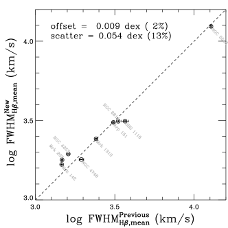
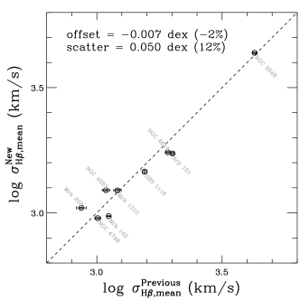
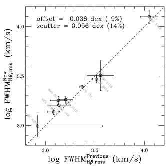
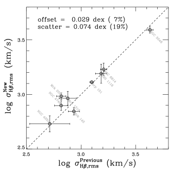
Figure 17.— Comparison of FWHM_Hβ (left) and $\sigma_{{\rm H}\beta}$ measurements (right) based on the new methods (this work) and the previous traditional methods (Bentz et al. 2009c), using the mean (top) and rms spectra (bottom). The average difference of the H$\beta$ line widths between two methods is relatively small. However, the large scatter (12–19%) indicates that the contribution from individual effects, e.g., subtraction of starlight, Fe II, or He II varies on an object-by-object basis.

5.2. Difference in Line Profile between SE and RMS spectra

We confirmed that the H$\beta$ line width measured from a mean or SE spectrum is systematically larger than that measured from an rms spectrum. The systematic difference corresponds to an average difference in virial product of $\sim$0.15–0.20 dex. However, the average difference is dominated by the narrowest line objects in the sample, with a decreasing trend toward broader line objects as shown in Fig. 15 (cf., Collin et al. 2006). These results indicate that for narrow-line AGNs (FWHM_Hβ $<3000$ km s^-1), BH masses based on SE spectra can be overestimated by $\sim$25–35% if standard recipes are used. In order to correct for the systematic difference of the line profile, we derive new empirically calibrated line-width dependent SE mass estimators.

It is important to notice that line-width measurements from rms spectra can also be systematically biased by residuals of narrow-line components, Fe II, and host-galaxy starlight. Fluctuations of these components can generate signatures in the rms spectra, resulting in a biased line profile and an improper continuum fit. We have demonstrated several new strategies to mitigate these effects. First, we adopt two robust methods to derive rms spectra — using S/N weights and adopting a maximum likelihood approach — that minimize the contamination of low-S/N spectra when there is a large range in S/N. Second, we subtract Fe II and host-galaxy starlight based on spectral decomposition analysis of each individual-epoch spectrum before making the rms and mean spectra. These new methods substantially improve the quality of rms spectra in measuring the width of the H$\beta$ line for AGNs with strong starlight, Fe II, or blended He II. Especially in these cases we recommend the new methods as an useful alternative to the traditional simple methods in future reverberation mapping studies (and possibly to revisit previous studies).

The new methods introduced here differ from previous ones. The overall goal is to account for systematic uncertainties and correct for biases stemming from known effects such as stellar line contamination. However, it is possible that they might introduce biases due to unknown systematics, especially when directly compared to other measurements obtained with previous techniques. An absolute comparison would require a third way to measure the same quantities (e.g., BH mass); however, we can estimate any differential bias by comparing our measurements to those given by Bentz et al. (2009c) using traditional methods. On average, $\sigma_{{\rm H}\beta}$ measured with our new methods increases by $7\pm 6$% and FWHM_Hβ increases by $9\pm 4$% (see Fig. 17), suggesting that the systematic uncertainties due to the new methods is lower than 10%, although we assume the difference is entirely caused by the systematic uncertainty of the new scheme.

The average small difference between our new measurements and those of Bentz et al. (2009c) is due to the fact that various effects, e.g., S/N weighting, prior subtraction of host galaxy starlight and blended emission lines, line profile fitting, and removal of narrow H$\beta$, are mixed together and canceled out for individual objects. For example, if we separate the effect of host galaxy starlight, the difference of the line dispersion measurements with/without removal of host galaxy starlight is much larger than the average difference between Bentz et al. (2009c) and ours (see §3.3.2). The 10-20% rms scatter between previous (Bentz et al., 2009c) and new measurements indicates that the contribution of each effect varies on an object-by-object basis (see Fig. 17). The new methods are useful for reducing the uncertianites of individual BH masses due to those various effects, and better constraining the intrinsic scatter of the $M_{\rm BH}-\sigma_{*}$ relation (e.g., Woo et al. 2010). When other systematic uncertainites, i.e., the virial coefficient, can be constrained and reduced in the future, the new methods will become more important for BH mass determination.

From the point of view of interpretation, the systematically narrower line width in the rms spectra can be explained by the photoionization calculations of Korista & Goad (2004), which predict that high-velocity gas in the inner BLR has lower responsivity, leading to lower variability of the line wings and therefore a narrower profile in the rms spectrum. However, it is not clear why the effect should be stronger for the narrower line AGNs. Further investigations are required to reveal the nature of this systematic trend. We conclude by noting that our study is limited to relatively low luminosity and narrow line width (and hence small BH mass) AGNs. In future work we plan to expand our study to cover a larger dynamic range in luminosity and line width.

5.3. Implications for the Evolution of BH Host-Galaxy Scaling Relations

Virtually all observational studies of the evolution of the BH host-galaxy scaling relations over cosmic time are based on SE mass estimates. Evolutionary trends are generally established by comparing measurement of distant samples (based on SE BH mass estimates) with the local scaling relations. The latter can be determined either based on SE BH mass estimates, or on reverberation BH mass estimates, or on spatially resolved kinematics. In the case of comparison between SE mass estimates at high redshift and mass estimates of local objects based on different methods, it is essential that the mass estimates be properly calibrated. For example, the positive bias of H$\beta$ line width of SE spectra compared to the rms spectra could lead to overestimation of BH masses for distant samples, if compared with local samples based on rms spectra.

However, as shown in Figures 13 and 14, this bias is only significant for the narrower line objects with BH mass $<10^{7}$ M_⊙). Typically, high-redshift studies such as those by Bennert et al. (2010) and Merloni et al. (2010) focus on higher mass BHs, where the bias is believed to be negligible. We note that one could completely eliminate this bias by comparing distant and local BH mass estimates based entirely on self-consistent SE BH mass estimates (Woo et al. 2008;Bennert et al. 2011a, b). Even then, of course, one must keep in mind the differential nature of the measurement. For example, the slope inferred for the local scaling relations based on SE spectra (e.g., Greene & Ho 2006) may be biased with respect to the true slope if the mass estimator is biased at low masses, and yet one may still infer the correct evolution even for low masses if the bias does not change with redshift.

References

- Barth et al. (2005) Barth, A. J., Greene, J. E., & Ho, L. C., 2005, ApJ, 619, L151
- Barth et al. (2011) Barth, A. J., et al. 2011, ApJ, 732, 121
- Bennert et al. (2010) Bennert, V. N., et al. 2010, ApJ, 708, 1507
- Bennert et al. (2011a) Bennert, V. N., et al. 2011a, ApJ, 726, 59
- Bennert et al. (2011b) Bennert, V. N., et al. 2011b, arXiv:1102.1975
- Bentz et al. (2006) Bentz, M. C., Peterson, B. M., Pogge, R. W., Vestergaard, M., & Onken, C. A. 2006, ApJ, 644, 133
- Bentz et al. (2009a) Bentz, M. C., Peterson, B. M., Pogge, R. W., & Vestergaard, M. 2009a, ApJ, 694, L166
- Bentz et al. (2009b) Bentz, M. C., et al. 2009b, ApJ, 697, 160
- Bentz et al. (2009c) Bentz, M. C., et al. 2009c, ApJ, 705, 199
- Brewer et al. (2011) Brewer, B. J., et al. 2011, ApJ, 733, L33
- Blandford & McKee (1982) Blandford, R. D., & McKee, C. F. 1982, ApJ, 225, 419
- Boroson & Green (1992) Boroson, T. A., & Green, R. F. 1992, ApJS, 80, 109
- Bruzual & Charlot (2003) Bruzual, G., & Charlot, S. 2003, MNRAS, 344, 1000
- Christiani et al. (1997) Cristiani, S., Trentini, S., La Franca, F., & Andreani, P. 1997, A&A, 321, 123
- Collin et al. (2006) Collin, S., Kawaguchi, T., Peterson, B. M., & Vestergaard, M. 2006, A&A, 456, 75
- Davies et al. (2006) Davies, R. I., et al. 2006, ApJ, 646, 754
- Davis et al. (2007) Davis, S. W., Woo, J.-H., & Blaes, O. M., 2007, ApJ, 668, 682
- Decarli et al. (2010) Decarli, R., Falomo, R., Treves, A., Labita, M., Kotilainen, J. K., & Scarpa, R., 2010, MNRAS, 402, 2453
- Denney et al. (2009) Denney, K. D., et al. 2009, ApJ, 692, 246
- Denney et al. (2010) Denney, K. D., et al. 2010, ApJ, 721, 715
- Dietrich et al. (2005) Dietrich, M., Crenshaw, D. M., & Kraemer, S. B., 2005, ApJ, 623, 700
- Ferrarese & Ford (2005) Ferrarese, L., & Ford, H. 2005, Space Sci. Rev., 116, 523
- Ferrarese & Merritt (2000) Ferrarese, L., & Merritt, D. 2000, ApJ, 539, L9
- Fine et al. (2008) Fine, S., et al. 2008, MNRAS, 390, 1413
- Gebhardt et al. (2000) Gebhardt, K., et al. 2000, ApJ, 539, L9
- Greene & Ho (2006) Greene, J. E., & Ho, L. C. 2006, ApJ, 641, 21
- Gültekin et al. (2009) Gultekin, K., et al. 2009, ApJ, 698, 198
- Hicks & Malkan (2008) Hicks, E. K. S., & Malkan, M. A. 2008, ApJS, 174, 31
- Hopkins et al. (2006) Hopkins, P. F., et al. 2006, ApJS, 163, 1
- Kaspi et al. (2005) Kaspi, S., Maoz, D., Netzer, H., Peterson, B. M., Vestergaard, M., & Jannuzi, B. T. 2005, ApJ, 629, 61
- Kaspi et al. (2000) Kaspi, S., Smith, P. S., Netzer, H., Maoz, D., Jannuzi, B. T., & Giveon, U. 2000, ApJ, 533, 631
- Kauffmann & Haehnelt (2000) Kauffmann, G., & Haehnelt, M. 2000, MNRAS, 311, 576
- Kelly (2007) Kelly, B. C., 2007, ApJ, 665, 1489
- Kollatschny (2003) Kollatschny, W., 2003, A&A, 407, 461
- Kollmeier (2006) Kollmeier, J., A., 2006, ApJ, 648, 128
- Kormendy & Richstone (1995) Kormendy, J., & Richstone, D. 1995, ARA&A, 33, 581
- Kormendy & Gebhardt (2001) Kormendy, J., & Gebhardt, K. 2001, in 20th Texas Symposium on Relativistic Astrophysics, ed. J. C. Wheeler & H. Martel (New York: AIP, vol. 586), 363
- Korista & Goad (2004) Korista, K. T., & Goad, M. R., 2004, ApJ, 606, 749
- Lauer et al. (2007) Lauerrconi, T., R., et al. 2007, ApJ, 670, 249
- Marconi & Hunt (2003) Marconi, A., & Hunt, L. K. 2003, ApJ, 589, L21
- Marconi et al. (2008) Marconi, A., et al. 2008, ApJ, 678, 693
- Magorrian et al. (1998) Magorrian, J. et al. 1998, AJ, 115, 2285
- Markwardt (2009) Markwardt, C. B. 2009, in Astronomical Data Analysis Software and Systems XVIII, ed. D. A. Bohlender, D. Durand, & P. Dowler (San Francisco: ASP), 251
- McGill et al. (2008) McGill, K. L., Woo, J.-H., Treu, T., & Malkan, M. A. 2008, ApJ, 673, 703
- McLure & Dunlop (2004) McLure, R. J., & Dunlop, J. S. 2004, MNRAS, 352, 1390
- Merloni et al. (2010) Merloni, A. et al. 2010, ApJ, 708, 137
- Onken et al. (2004) Onken, C. A., Ferrarese, L., Merritt, D., Peterson, B. M., Pogge, R. W., Vestergaard, M., & Wandel, A. 2004, ApJ, 615, 645
- Netzer & Marziani (2010) Netzer, H., & Marziani, P. 2010, ApJ, 724, 318
- Onken et al. (2007) Onken, C. A., et al. 2007, ApJ, 670, 105
- Pancoast et al. (2011) Pancoast, A., Brewer, B. J., & Treu, T. 2011, ApJ, 730, 139
- Peng et al. (2006) Peng, C. Y., Impey, C. D., Rix, H.-W., Kochanek, C. S., Keeton, C. R., Falco, E. E., Lehár, J., & McLeod, B. A. 2006, ApJ, 649, 616
- Peterson (1993) Peterson, B. M., 1993, PASP, 105, 247
- Peterson & Wandel (1999) Peterson, B. M., & Wandel, A., 1999, ApJ, 521, L95
- Peterson & Wandel (2000) Peterson, B. M., & Wandel, A., 2000, ApJ, 540, L13
- Peterson et al. (2004) Peterson, B. M., et al. 2004, ApJ, 613, 682
- Robertson et al. (2006) Robertson, B. et al. 2006, ApJ, 641, 90
- Sergeev et al. (1999) Sergeev, S. G., Pronik, V. I., Sergeeva, E. A., Malkov, Yu. F. Sergeev, S. G., Pronik, V. I., Sergeeva, E. A., & Malkov, Yu. F., 1999, AJ, 118, 2658
- Shapovalova et al. (2004) Shapovalova, A. I., et al. 2004, å, 422, 925
- Shen et al. (2008) Shen, Y., Greene, J. E., Strauss, M. A., Richards, G. T., & Schneider, D. P. 2008, ApJ, 680, 169
- Shen & Kelly (2010) Shen, Y., & Kelly, B. C., 2010, ApJ, 713, 41
- Shen et al. (2011) Shen, Y., et al. 2011, ApJS, 194, 45
- Shields et al. (1995) Shields, J. W., Ferland, G. J., & Peterson, B. M. 1995, ApJ, 441, 507
- Tremaine et al. (2002) Tremaine, S., et al. 2002, ApJ, 574, 740
- Treu et al. (2007) Treu, T., Woo, J.-H., Malkan, M. A., & Blandford, R. D. 2007, ApJ, 667, 117
- van Groningen & Wanders (1992) van Groningen, E., & Wanders, I. 1992, PASP, 104, 700
- van der Marel & Franx (1993) van der Marel, R. P., & Franx, M. 1993, ApJ, 407, 525
- Vanden Berk et al. (2001) Vanden Berk, D. E., et al. 2001, AJ, 122, 549
- Vestergaard & Peterson (2006) Vestergaard, M., & Peterson, B. M. 2006, ApJ, 641, 689
- Wandel et al. (1999) Wandel, A., Peterson, B. M., & Malkan, M. A. 1999, ApJ, 526, 579
- Wilhite et al. (2007) Wilhite, B. C., Brunner, R. J., Schneider, D. P., & Vanden Berk, D. E. 2007, ApJ, 669, 791
- Woo & Urry (2002) Woo, J.-H., & Urry, M., 2002, ApJ, 579, 530
- Woo et al. (2004) Woo, J.-H., Urry, C. M., Lira, P., van der Marel, R. P., & Maza, J., 2004, ApJ, 617, 903
- Woo et al. (2006) Woo, J.-H., Treu, T., Malkan, M. A., & Blandford, R. D. 2006, ApJ, 645, 900
- Woo et al. (2007) Woo, J.-H., Treu, T., Malkan, M. A., Ferry, M. A., & Misch, T. 2007, ApJ, 661, 60
- Woo et al. (2008) Woo, J.-H., Treu, T., Malkan, M. A., & Blandford, R. D., 2008, ApJ, 681, 925
- Woo et al. (2010) Woo, J.-H., et al. 2010, ApJ, 716, 269