Thinking Outside the Box:
Effects of Modes Larger than the Survey on
Matter Power Spectrum Covariance
Abstract
Accurate power spectrum (or correlation function) covariance matrices are a crucial requirement for cosmological parameter estimation from large scale structure surveys. In order to minimize reliance on computationally expensive mock catalogs, it is important to have a solid analytic understanding of the different components that make up a covariance matrix. Considering the matter power spectrum covariance matrix, it has recently been found that there is a potentially dominant effect on mildly non-linear scales due to power in modes of size equal to and larger than the survey volume. This beat coupling effect has been derived analytically in perturbation theory and while it has been tested with simulations, some questions remain unanswered. Moreover, there is an additional effect of these large modes, which has so far not been included in analytic studies, namely the effect on the estimated average density which enters the power spectrum estimate. In this article, we work out analytic, perturbation theory based expressions including both the beat coupling and this local average effect and we show that while, when isolated, beat coupling indeed causes large excess covariance in agreement with the literature, in a realistic scenario this is compensated almost entirely by the local average effect, leaving only of the excess. We test our analytic expressions by comparison to a suite of large N-body simulations, using both full simulation boxes and subboxes thereof to study cases without beat coupling, with beat coupling and with both beat coupling and the local average effect. For the variances, we find excellent agreement with the analytic expressions for Mpc-1 at , while the correlation coefficients agree to beyond Mpc-1. As expected, the range of agreement increases towards higher redshift and decreases slightly towards . We finish by including the large-mode effects in a full covariance matrix description for arbitrary survey geometry and confirming its validity using simulations. This may be useful as a stepping stone towards building an actual galaxy (or other tracer’s) power spectrum covariance matrix.
I Introduction
Galaxy surveys (and surveys of other dark matter tracers) are an important tool for constraining cosmological parameters and the tracer’s power spectrum (or its Fourier transform, the correlation function) is the most valuable observable. It can be used to measure the scale of baryon acoustic oscillations (BAO, see e.g. Seo and Eisenstein (2003); Eisenstein et al. (2005); Cole et al. (2005); Blake et al. (2011)), which is a particularly robust feature and a strong probe of dark energy through the measurement’s dependence on the expansion history, but it is also common to use the full shape of the power spectrum to constrain cosmology (e.g. Efstathiou et al. (2002); Reid et al. (2010)). In order for these measurements to be useful for cosmology however, it is crucial to have an accurate estimate of the observable’s covariance matrix. As surveys get larger, calculating such a matrix directly from simulations becomes ever more challenging. In fact, large numbers of mock catalogs are required to estimate covariance matrices directly from simulations and it is computationally very costly to create such numbers with the required volume and resolution. Moreover, the covariance matrix is cosmology dependent so ideally one would either be able to generate a large number of matrices for different cosmologies, or show that this cosmology dependence can be safely neglected. This requirement increases the number of mocks needed in the brute force method even further. It is therefore important to develop a good analytical understanding in order to eventually rely less on simulations.
While the density of tracers may have a non-trivial relation with the dark matter density, a good first step towards understanding the true covariance matrix is to study that of the dark matter power spectrum. The two main complications in understanding the dark matter matrix are the mode mixing due to the finite survey volume and the non-Gaussian nature of the matter overdensity field on small scales (Mpc-1) due to non-linear evolution. While the former is relatively straightforward to quantify (Feldman et al. (1994)), the latter effects are the subject of a large number of studies Scoccimarro et al. (1999); Meiksin and White (1999); Cooray and Hu (2001); Scoccimarro and Sheth (2002); Sirko (2005); Sefusatti et al. (2006); Neyrinck et al. (2006); Neyrinck and Szapudi (2007); Smith (2009); Sato et al. (2009); Neyrinck (2011); Harnois-Deraps and Pen (2011); Ngan et al. (2011), involving N-body simulations, perturbation theory and the halo model. For covariances on non-linear scales, an important (but often overlooked) role is played by modes of wavelength comparable to and larger than the survey size. In particular, Hamilton et al. (2006); Rimes and Hamilton (2006) found that the interplay of mode mixing by the survey window with non-linear correlations between a pair of small-scale modes and a large mode, causes a covariance contribution proportional to the power in super-survey modes, and that, in fact, this is the dominant contribution to the covariance matrix on small scales. The added covariance affects both the variances and the off-diagonal covariances. This effect is usually called beat coupling (see also Sefusatti et al. (2006); Takada and Jain (2009); Reid et al. (2009); Takahashi et al. (2009)). A second consequence of the presence of modes larger than the survey is that the average density (which is needed to construct the overdensity) estimated from the survey has a variance itself, leading to an additional covariance contribution proportional to the large scale power. We will refer to this as the local average effect.
In the standard approach to estimating covariances from N-body simulations, the power spectrum is calculated using the full, periodic simulation volume. However, this completely misses the large effects discussed above because there are no modes larger than the “survey” volume. In order to capture these effects, one thus needs to consider either a subvolume of a (much) larger simulation, or implement a varying zero mode (Sirko (2005)) in the simulations. While some such studies have been performed (see e.g. Takahashi et al. (2009); Reid et al. (2009)), a systematic study, leading to a complete and well tested analytic description has until now been lacking.
In this article, we aim to present such a study. We use a set of large (Mpc) N-body simulations and study the aforementioned effects of large modes by considering significantly smaller subboxes (Mpc), thus imitating the real world scenario of a finite survey embedded in an infinite universe. We build an analytic model for the covariance matrix, properly including the effect of the window function and describing non-linear effects using perturbation theory. This description includes the beat coupling model from Hamilton et al. (2006), but adds to this an analytic estimate of the local average effect. The latter effect needs to be included when building a covariance matrix for a realistically estimated power spectrum and has to our knowledge not been calculated analytically previously.
We compare our model to simulations at five redshifts in the range and generally find excellent agreement until well into the non-linear regime. Since we test several combinations of covariance matrix contributions individually by employing different approaches to estimating spectra from simulations, we are confident that our theoretical understanding of the dark matter covariance is correct and that we have captured the main effects.
One of our main results is that, while beat coupling indeed causes excess covariance which soon dominates, the contribution from the local average effect cancels most of this out, leaving only a reduced beat coupling contribution of about of the original.
In addition to the effects on non-linear scales discussed above, the mode mixing due to the window function also has a well known effect on linear scales, correlating neighboring power spectrum estimators and reducing the variances. This effect needs to be taken into account for a realistic survey. We calculate these covariances directly using analytic expressions from Feldman et al. (1994) and show good agreement with simulations. Thus, while the main goal of this paper is to study the beat coupling and local average effects related to super-survey modes, we also provide a complete expression that can be used to calculate a (dark matter) covariance matrix for an arbitrary survey geometry and can serve as a stepping stone for calculating a galaxy (or other dark matter tracer) spectrum covariance matrix. We also study the cosmology dependence of the covariance matrix and find that for cosmological parameter variations relevant to current cosmological constraints, the covariance matrix undergoes changes at the level.
The outline of this article is as follows. We explain the analytic description of the covariance matrix in section II, using a simple formalism apt for the description of simulation results. This will lead to three expressions that can be tested against simulations (without beat coupling, with beat coupling, and with beat coupling and local average effect). We then describe our N-body simulations in section III and compare the results to theory in section IV. While for the main results in this paper, we stick to a simple description in terms of a discrete set of modes, we discuss a more rigorous and complete treatment of the window function in section V, leading to expressions that can be applied to arbitrary survey geometry. We conclude and summarize our work in section VI. Finally, we use our analytic expressions to briefly discuss the cosmology dependence of the covariance matrix in the Appendix.
As this article is rather long and technical, we provide some recommendations for a reader on a tight schedule. On a first reading, this reader may want to skip the mathematical discussion in section II and jump straight to section II.5, where the main equations are summarized. Moreover, in section V, one could jump to Eq. (48), which presents the final covariance matrix expression for general geometry, and then focus on the results in Figs 6-9, where the green points and lines show the covariance matrix corresponding to said equation.
II Covariance Matrix Formalism
In this section, we work out the formalism for calculating a covariance matrix for a power spectrum measured from a cubic volume with uniform selection function, i.e. the geometry of N-body simulations. We describe the density field in terms of a discrete set of modes, which significantly simplifies notation. We will provide a more general description, which can be applied to an arbitrary survey geometry (following Feldman et al. (1994)), in section V. The more technical discussion there also serves to motivate the simpler approach taken in this section.
II.1 N-body Simulation Geometry (Cubic Box)
We consider a cubic subvolume of the universe (which later in this article will be modeled by taking a subvolume of a much larger periodic simulation box). The matter overdensity field , where is the matter density and its mean, can be expanded as
| (1) |
To significantly simplify notation, we choose to describe the density field in the volume in terms of discrete Fourier modes in analogy to the usual description of the density field in a periodic box, i.e. we effectively describe the field in the subvolume by
| (2) |
To be more exact, we define the discrete modes as
| (3) |
In other words, is equal to the FKP estimator (Feldman et al. (1994)) (up to a factor ) applied to the volume , and is therefore a weighted average over a range of continuum Fourier modes. In particular, while there is no true mode, the subvolume sees an effective zero mode (see also Sirko (2005)) which gets its main contribution from continuum Fourier modes . Note that Eq. (2) is not to be taken literally, as the field is not actually periodic with respect to the volume . We discuss the effect of taking a subvolume more rigorously in section V.
The statistics of the discrete overdensity modes can be characterized by a sequence of connected point functions,
| , |
where we have defined the power spectrum , bispectrum an the trispectrum . Note that these are technically weighted averages of the true, continuum power, bi- and trispectrum, for example (see also section V)
| (4) |
where is the zeroth spherical Bessel function.
The power of an individual mode can be estimated as
| (5) |
such that as desired, from which one can define a bin averaged estimator in order to maximize signal to noise,
| (6) |
Here, the sum is over all , with integer components , such that lies in some small range defining the -th bin. is the number of modes in . The expectation value , with a typical mode inside the bin.
We are interested in the covariance matrix of this bin averaged estimator,
| (7) |
Starting from the covariances in the individual mode estimators,
| (8) |
we obtain
| (9) |
where we have introduced the shorthand notation for the bin averaged trispectrum. The term proportional to the power spectrum squared is diagonal and given by simply counting modes because the binning in -space only includes pairs of estimators that have zero covariance. As we will discuss in detail in section V, this is not in general the case as the window function may correlate different bins.
II.2 N-body Simulation Geometry: Perturbation Theory
The power spectrum appearing in the first term on the right hand side of Eq. (9) is the full non-linear power spectrum, which can be estimated directly from simulations. The trispectrum is harder to get from simulations (but see Harnois-Deraps and Pen (2011)), but can be modeled using a variety of perturbation theory schemes or using the halo model. In this work, we will use the simple framework of (Eulerian) standard perturbation theory (SPT; Bernardeau et al. (2002); Fry (1984); Goroff et al. (1986); Scoccimarro et al. (1999)). Anticipating angle averaging, i.e. modulo transformations and , the leading order trispectrum for the configuration of interest is given as (see111Note that the factor in Eq. (7) of Scoccimarro et al. (1999) should be a factor . Fry (1984); Scoccimarro et al. (1999))
| (10) |
where and are the kernels for the second and third order contributions to the density field, as given in the appendix of Goroff et al. (1986). We can now distinguish two types of terms. The first two lines represent the “standard” trispectrum contributions, that have always been included in PT studies of the trispectrum (see e.g. Scoccimarro et al. (1999)). When no modes larger than the survey are present, like in the artificial case of a power spectrum estimated from the full volume of a periodic (N-body simulation) box, these are the only terms entering the trispectrum, giving
| (11) |
We will evaluate numerically as no further analytic simplifications are possible.
II.3 The Beat Coupling Effect
The third line in Eq. (II.2) is the beat coupling contribution, the importance of which has been realized only more recently (Hamilton et al. (2006); Takahashi et al. (2009); Takada and Jain (2009); Reid et al. (2009); Rimes and Hamilton (2006); Sefusatti et al. (2006)). Our notation here requires some explanation (see also section V). Consistent with our discussion in the previous section, quantities evaluated at should really be interpreted in terms of an effective zero mode arising from contributions at , i.e. , generated by continuum contributions with . Moreover, , given by
| (12) |
is at first sight not well defined if one of the arguments equals . (and the other affected term) should thus be interpreted as a limit
| (13) |
with (see section V for a more rigorous treatment of the beat coupling term with the same result). The integral over the direction of makes this quantity well defined.
Using the fact that
| (14) |
the beat coupling term can be angle (or bin) averaged analytically so that we end up with
| (15) |
Physically, the presence of the beat coupling term is an interesting interplay of mode mixing due to the window functions with correlations between pairs of non-linear modes and one larger mode (see Hamilton et al. (2006)). Due to the finite volume from which the power spectrum is measured, the estimator really consists of a weighted average of pairs of density modes , with of order of the fundamental mode . For in the non-linear regime, such pairs correlate with the large scale perturbation , which in turn causes the covariance between the power spectrum estimators to be proportional to the power in these large modes. In our description, this is captured by the power in the effective zero mode. Note that the beat coupling creates an excess both in the variance and in the off-diagonal elements of the covariance matrix.
II.4 The Local Average Effect
While the beat coupling term derived in the previous section adds significant covariance on non-linear scales, there is an additional effect coupling small scale covariance to power in the zero-mode that plays a role in the power spectrum estimated from an actual survey. This second effect is caused by the fact that to obtain the overdensity , one needs an estimate of the average density . In a realistic survey, one does not know the true average number density of, say, galaxies, but instead has to rely on an estimate of the average density within the survey volume, which is modulated by the zero mode . This results in a decrease in covariance, partially canceling the beat coupling effect222The difference between using the true and the local average was also commented on briefly in Neyrinck et al. (2009). We will refer to this contribution as the local average effect.
The local average effect causes the true overdensity estimator to be given by
| (16) |
Since also appears in the numerator of , there technically is also a contribution there. However, the Fourier transform of the zero mode for non-zero wave vector vanishes so this term can be omitted. Eq. (16) can be expanded in powers of to derive expressions for the -point functions to the desired order in perturbation theory. For example, to next-to-leading order, the expectation value of the power spectrum estimator becomes
| (17) | |||||
The expectation value of the angle-averaged estimator is then
| (18) | |||||
Hence, the power spectrum receives a small bias due to the local average effect. The relative correction is for a 1Gpc3 survey so it can be safely ignored for a realistic survey. Here, we have used that the bispectrum (Sefusatti et al. (2006))
| (19) |
and we have applied the identity (14) to carry out the angle averaging.
Using the same approach for the covariance matrix, one gets to next to leading order
| (20) |
where we have ignored a small relative correction to the diagonal term of order . The local average effect thus introduces a term of the same form as the beat coupling term from the previous section, proportional to , but with opposite sign. Comparing the coefficients, one finds that the two effects almost entirely cancel out, leaving only a small positive coefficient, of the original beat coupling coefficient. Note that the local average effect to this order consists of contributions from the bispectrum and trispectrum, but also from terms that would even be there had the field remained completely Gaussian (but that happen to be of the same order as the leading non-Gaussian corrections).
Eq. (20) thus gives us an expression for the most realistic case we will consider, where modes larger than the survey are present and the spectrum is estimated using the local average in the survey volume.
II.5 Theory Summary and Outlook
In the remainder of this article, we will use N-body simulations to test the expressions derived above. We will consider three different cases which allow us to separately constrain different combinations of contributions to the total covariance:
-
•
Case 1: periodic box
The spectrum is estimated from the full, periodic simulation volume. In this case, there is no beat coupling nor a local average effect and the prediction for the covariance is to leading order(21) We obtain the (non-linear) power spectrum appearing above by applying the Halofit333We have checked that the difference between using the Halofit spectrum and the average simulated spectrum is small for Mpc. prescription Smith et al. (2003) to the linear power spectrum calculated using CAMB Lewis et al. (2000). The bin-averaged trispectrum is given by Eq. (11), where we make one modification. Instead of using the linear power spectra, we use the non-linear spectra. This is consistent to the desired order in perturbation theory and turns out to slightly improve the accuracy of the model on strongly non-linear scales.
-
•
Case 2: subbox of periodic box
Since modes larger than the “survey volume” are now present, there is a beat coupling effect. The leading order covariance prediction is(22) Note that also for the additional trispectrum terms, we choose to use the non-linear power spectrum as opposed to the linear one.
-
•
Case 3: subbox of periodic box, using subbox mean
This is the most realistic case, where not only there are modes larger than the survey, but the overdensity is calculated in terms of the average density of the subbox, as opposed to the “true” average density of the full box. The leading order part of the covariance matrix is given by(23)
In the next section, we first describe the details of our simulations. We will discuss the results of our comparison in section IV.
III N-body simulations
In order to test our analytic predictions we use a large suite of N-body simulations. We have two sets of simulations consisting of 160 runs of a Mpc box with particles and 1024 runs of a Mpc box with particles. The initial conditions of the 160 and 1024 simulations were set up using different realizations of a Gaussian random field with the power spectrum given by CAMB. We adopted a flat CDM cosmology consistent with the current observational constraints Komatsu et al. (2010). The cosmological parameters are the present-day matter fraction , Hubble constant , baryon fraction , spectral index , and present-day normalization .
The particles were displaced from their initial grid points according to second-order Lagrangian perturbation theory using an initial redshift .
The simulations were performed with the Tree-PM code Gadget-2 Springel (2005) taking only the gravitational force into account. We applied a force softening of kpc and used a particle mesh of and for the Mpc and Mpc runs, respectively. Using a much higher resolution simulation, we checked that with these simulation settings the power spectrum derived from the simulation data is accurate at the 1% level up to and remains accurate within 4% up to at all redshifts.
To compute the power spectrum from the simulation data, we assign the particles using the cloud-in-cell (CIC) scheme to a regular grid with a fixed grid spacing of Mpc in all cases (full box, subbox, subbox with zero-padding). Hence, the Nyquist frequency of the grid is the same in all cases, Mpc, which is 5 times larger than the scales we consider in this paper . Therefore we expect the effects due to finite grid size (smearing and aliasing effects) to be very small. Nevertheless, we do correct for the smearing due to the CIC assignment Jing (2005).
The simulations and the power spectrum computation needed about CPU hours on our in-house cluster Hipatia at ICCUB.
IV Results
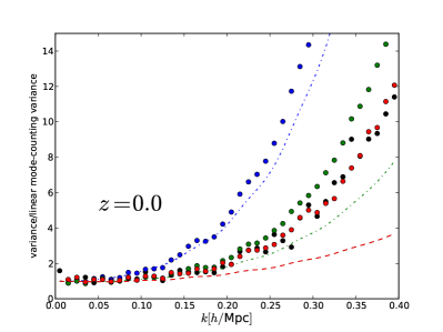
We now compare the simulation results to the analytic predictions summarized in section II.5. For the covariances of the full periodic box (Case 1), we compare to the 1024 simulations of the Mpc cubed volume and to the 160 simulations of the Mpc cubed volume. To study the subbox Cases 2 & 3, we divide the Mpc volume into 64 smaller boxes with side Mpc each, which provides us with different subbox realizations.
For each volume, we estimate the power spectrum in isotropic bins of width in the range . We then estimate the covariance matrix for the full box, or for a particular subbox of it, by
| (24) |
where the sum runs over all simulation realizations and is the average power spectrum over simulations. In the subbox case, we then improve the accuracy by averaging the subbox covariance estimate in Eq. (24) over all 64 subboxes. Note that, since the subboxes living in the same simulation volume are not independent, it would be wrong to directly apply Eq. (24) to all subboxes.
Since the non-linear effects discussed in section II become stronger with time, it is interesting to consider the covariance matrix for a range of redshifts from . We expect our analytic predictions to have the largest range of validity at , as non-linear effects there are smallest.
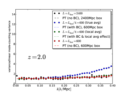
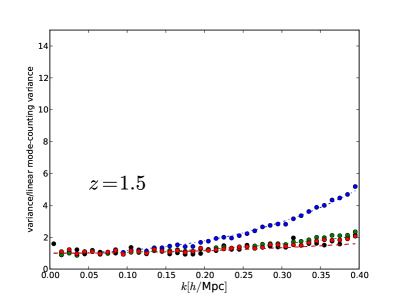
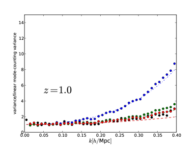
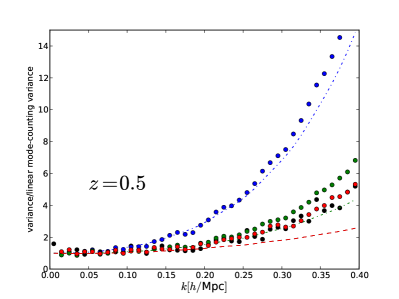
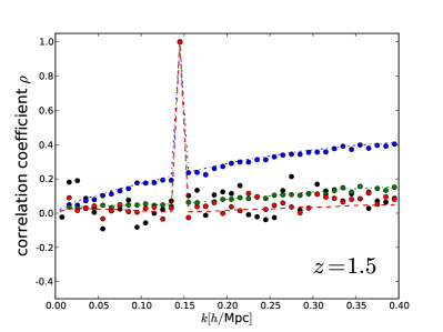
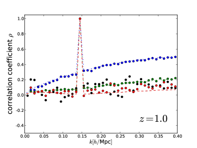
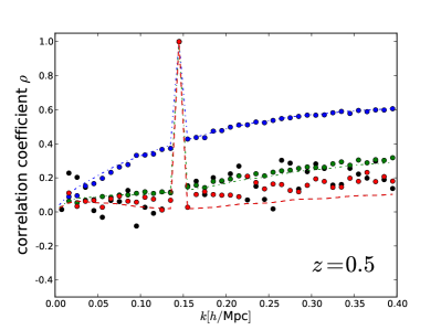
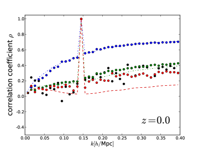
In Fig. 1, we show results for the variances in the power spectrum, normalized by the variance based on mode counting and the linear power spectrum. Case 1 is tested by both the full Mpc box case (black dots - N-body results, black dashed - analytic) and the full Mpc box case (red). The blue dots and dashed lines test Case 2 and the green ones test Case 3. For all cases and at all redshifts, we find good agreement between theory and simulation for bins up to a maximum value that lies in the non-linear regime. The values for are reasonable given the range of scales over which perturbation theory is expected to be applicable, at to at .
We now comment on the three scenarios of interest individually.
-
•
Case 1: periodic box
The Mpc and Mpc full-box simulation results agree very well with each other, as expected because they are both described by Case 1 and have no beat coupling. They also agree well with the analytic prediction. This confirms that excess covariance is not simply caused by the mere presence of large modes. The following two cases show that what matters is the presence of modes larger than the “survey” volume. -
•
Case 2: subbox of periodic box
Beat coupling introduces a large amount of excess variance and is well described by perturbation theory (for the range of scales discussed above). -
•
Case 3: subbox of periodic box, using subbox mean
As expected from theory, the local average effect undoes most of the excess variance due to beat coupling. Given the noise in the simulation results, the Case 3 simulation results do not distinguish with much significance the Case 3 theory prediction from the Case 1 prediction (but certainly from the Case 2 prediction). However, the Case 3 simulation results do clearly display a larger variance than the Case 1 results at large , looking consistent with having of the beat coupling excess variance.
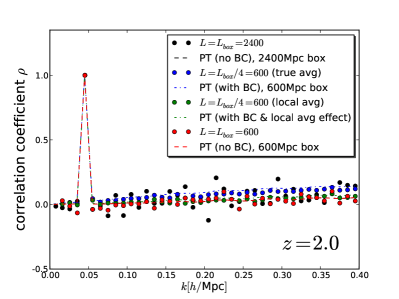
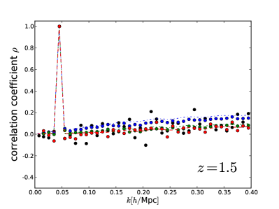
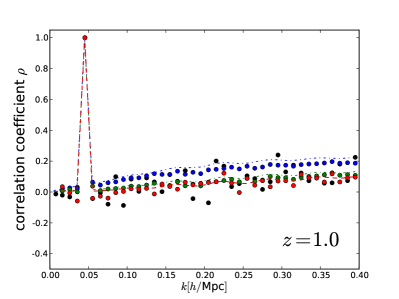
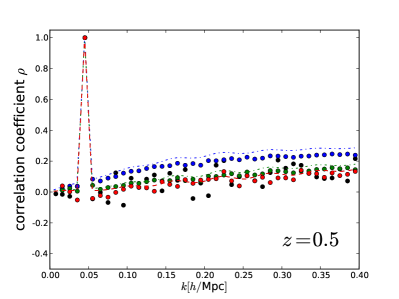
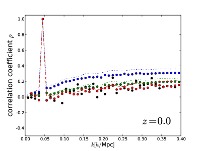
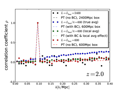
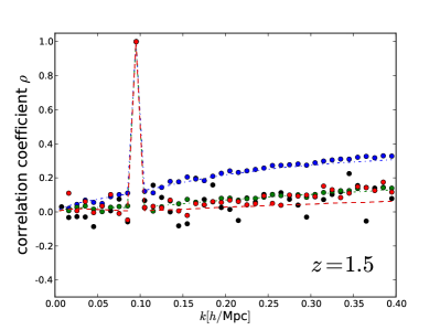
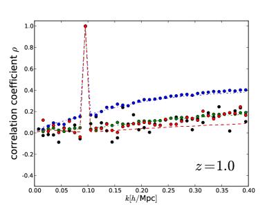
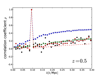
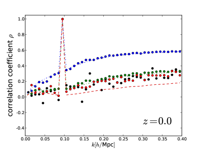
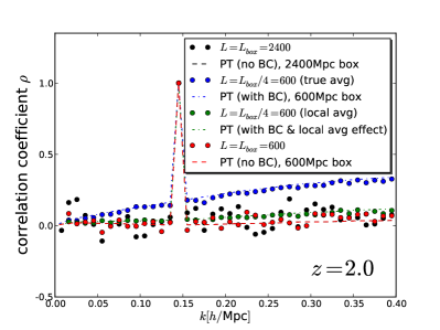
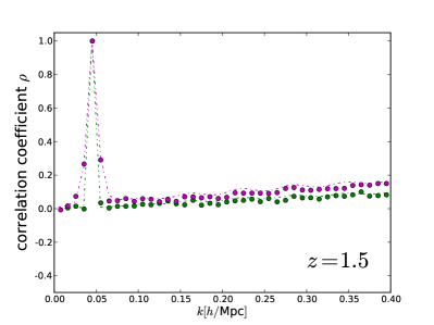
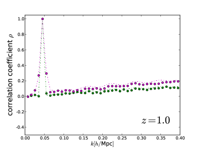
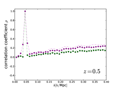
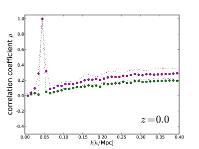
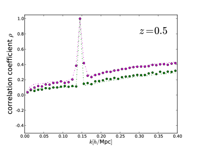
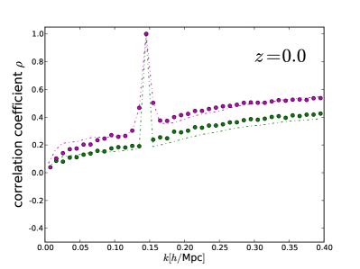
In Figs. 2 - 4, we quantify the off diagonal correlations by plotting the correlation coefficients between bins,
| (25) |
where we keep one bin fixed and let the value of corresponding to the other one vary on the horizontal axis. The fixed bins are at (Fig. 2), (Fig. 3) and (Fig. 4).
The conclusions for the correlation coefficients are similar to those drawn about the variances and again the analytic and numerical results agree well. In fact, for Cases 2 & 3, there now is good agreement up to Mpc-1 for all redshifts. We do note that the correlations relative to the bin appear to be overestimated somewhat by the analytic expressions. However, this is because the variance from simulations in the bin is somewhat high due to noise. Since this variance appears in the denominator of Eq. (25), it brings the simulation correlation coefficients down, thus explaining the slight disagreement with the analytic result. The other deviation is that the correlation coefficients relative to the bins at wave number ( and ) are higher than expected for Case 1 at low redshift. Whereas they should theoretically not have a beat coupling contribution, these correlation coefficients behave as if they do get such a contribution similar to the one in the scenario with beat coupling and the local average effect (Case 3). This may simply be due to non-linear effects beyond the order included in our theoretical expressions. Other than this, the agreement is very good.
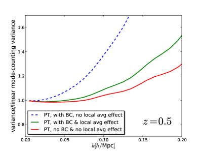
To conclude this section, we use our analytic expressions to quantify the importance of non-linear corrections to the covariance matrix on a range of scales relevant to large scale structure surveys. In the left panel of Fig. 5, we show the theory based variance, at redshift zero, taking into account all non-linear effects (green), and taking into account everything except for the beat coupling and local average effects (red). The figure is the same as in Fig. 1, except that the focus is on the theory curves in the range Mpc. We see that the full non-linear corrections change the variance at the level at Mpc and by at Mpc. For comparison, we also show in dashed blue the variance if we do not take into account the reduction in excess variance due to the local average effect. Neglecting to take the latter effect into account would lead to a gross overestimate of the non-linear variance.
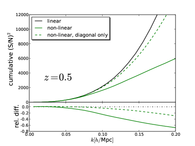
To quantify the effect of not only the non-linear corrections to the diagonal of the covariance matrix, but also of the non-diagonal elements, we next calculate the squared signal-to-noise ratio,
| (26) |
The sum here is over all pairs of power spectrum bins with both central values below . For , we use the (non-linear) power spectrum in the fiducial model, so that can be thought of as a detection (or amplitude) signal-to-noise. The top figure of the right panel of Fig. 5 shows this statistic using a (diagonal) linear covariance matrix (based on mode counting; black curve), the full non-linear matrix (green), and the non-linear matrix with the off-diagonal elements set to zero (dashed green). The bottom figure shows the relative difference with the linear signal-to-noise squared. Compared to the linear case, the non-linear, but diagonal covariance matrix indeed decreases the signal-to-noise, as expected from the increase in variance seen in the right panel. However, the off-diagonal elements have a significantly stronger effect and decrease the signal-to-noise even further. The signal-to-noise gives an idea of how much Fisher matrix elements in a parameter forecast, or values in a Monte Carlo chain, are affected by the non-linear corrections to the covariance matrix. This means that when a power spectrum study, whether with real data or in a Fisher forecast, includes modes well into the non-linear regime, it is not enough to just include non-linear corrections into the variance of the power spectrum. Instead, the full non-linear covariance matrix needs to be taken into account.
V General Survey Geometry
So far, we have found it convenient to describe the statistics of the density field in terms of a discrete set of overdensity modes. Whereas this is exact when considering the modes of a full periodic box, this should be considered an effective description in the case of subboxes, justified by their simple geometry. In this section, we work out the formalism for a general survey geometry in terms of the continuum of Fourier modes that exist in an infinite universe. We closely follow the notation and results of Feldman et al. (1994), but will add to this the trispectrum contributions arising in perturbation theory. The discussion in this section will provide justification for the discrete description of the previous sections. One issue that we will pay particular attention to is the motivation for using the diagonal mode-counting expression for the disconnected part of the covariance matrix in Eq. (9). As we will see, in the FKP formalism, the window function correlates power spectrum estimators in different bins (even in the Gaussian case), and the mode counting expression is not accurate. We will explain why mode counting was justified in the previous sections, argue that for a realistic survey the FKP description including cross correlations is the relevant one, and finally test the latter description against simulations.
We first define our Fourier convention as
| (27) |
The statistics of the continuum of Fourier modes are given by
| (28) | |||||
For a survey with background number density , consider then the weighted density field
| (29) |
where is a weight function that can be chosen to maximize signal to noise. We will ignore shot noise in the following, but it is straightforward to include it in the Gaussian approximation (see FKP). The Fourier transform is given by , where “” indicates a convolution, and the power spectrum can be estimated by , so that
| (30) |
The measured power spectrum is thus a weighted average of the true spectrum, with a weight function of width of order the fundamental mode of the survey, i.e. if is the typical scale of the survey. As a relevant example, the window function for a cubic box of side (, inside the box and zero outside) is given by
| (31) |
with the zeroth spherical Bessel function. If the true spectrum varies little across this range of scales, we get
| (32) |
V.1 Covariances - disconnected (Gaussian) contribution
We first consider the contribution to the covariance between FKP power spectrum estimators arising from products of two-point functions. This is the only contribution for a Gaussian density field and we can follow FKP for its description.
We start from the two-point function
| (33) |
where the second equality is true in the same limit where the (expectation value of the) power spectrum estimator equals the true spectrum, and is the Fourier transform of the (normalized) squared window function,
| (34) |
Hence, the covariance
| (35) |
In FKP, the power spectrum in a bin is given by
| (36) |
where is the -volume of bin , so that the covariance between (isotropic) bins is
| (37) |
Because of the extended nature of the window function , there will thus be correlations between different bins. In the limit that the bin width is much larger than the width of this window function, these correlations are negligible and one can make a further simplification by integrating out . Using
| (38) |
one ends up with
| (39) |
where is a typical mode in the -th bin and we have further assumed that the power spectrum varies little across a bin. This is the well know mode-counting result. The expression for the effective volume is further simplified in FKP by choosing an optimal weight function, but we will stick to general . Note that for our cubic box (or any other geometry with constant background number density and weighting), .
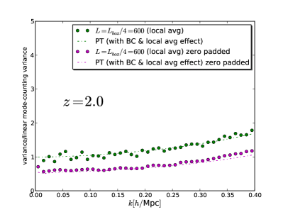
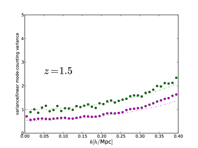
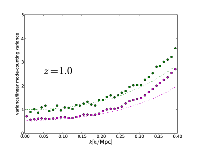
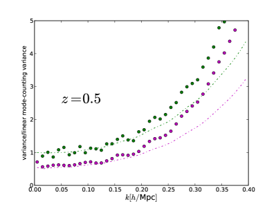
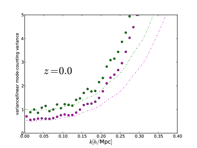
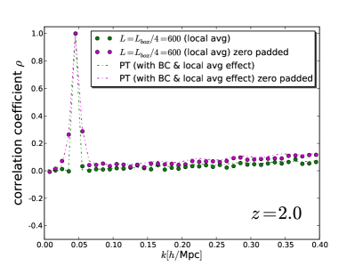
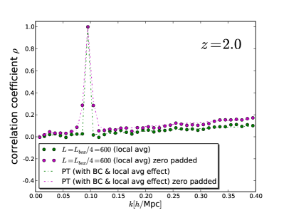
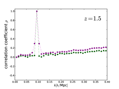
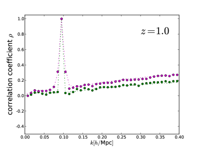
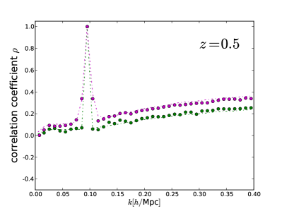
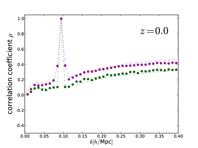
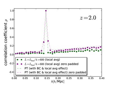
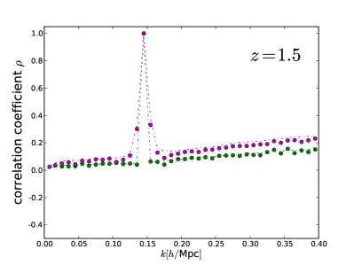
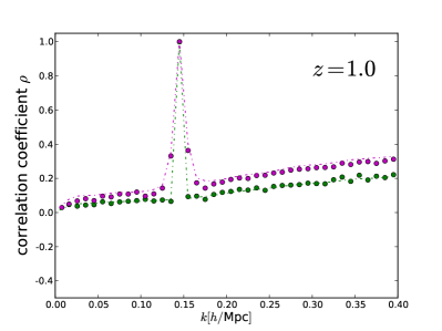
Assuming that embedding our Mpc cubed box in a Mpc cubed periodic box is a good approximation to embedding it in an infinite universe with a continuum of Fourier modes, we can apply the above to our simulated scenario and find that for our bin width Mpc-1, there should be significant correlations between bins and the mode-counting argument is not valid, in fact overpredicting the variances. We show this in figures 6 - 9, dashed lines, which we will discuss in more detail below.
Why then was it correct to use the diagonal, mode-counting expression in the previous sections? The reason is that, in keeping with our effective periodic box description, our bin average only includes modes which are multiples of the subbox’s fundamental mode, i.e. with the components of integers,
| (40) |
This decorrelates the binned power spectrum estimators as the mode mixing kernel
| (41) |
vanishes for separations that are a non-zero multiple of . Since the kernel equals unity for zero separation, the covariance in this averaging scheme is given by the mode-mixing result,
| (42) |
This begs the question if a similar binning scheme can be applied to an actual survey, in order to decorrelate power spectrum estimates in different bins. Unfortunately, for a realistic survey, the geometry will be much more complicated than a simple cube, making this rather difficult. In practice, therefore, one would typically embed the survey in a much larger cubic volume (zero-padding the part not covered by the survey), apply a Fourier transform, estimate the power spectrum for each on the grid by the embedding box (i.e. modulo with the size of the large box), and finally average to obtain the binned spectrum. This is thus a much denser sampling than the one we applied previously and approaches the infinitely dense FKP bin average of Eq. (36). In a more realistic scenario therefore, mode counting would not be sufficient and the off diagonal covariances are significant.
For this reason, it is useful to numerically test the mode mixing in the covariance matrix due to the window function as given in Eq. (37). We do this by again calculating the covariance matrix for our Mpc subbox, but this time using a binned spectrum averaged over all multiples of the fundamental mode of the large Mpc simulation box, thus increasing the sampling density by a factor of and approaching the FKP bin average. In practice, we zero-pad the exterior of the subbox and then apply the Fourier transform to the full box. The results are shown in figures 6 - 9 and compared to the analytic expression (37). To model the inevitable non-linear effects, we add trispectrum contributions to the theory prediction, which we will describe in the next subsection. Even without these contributions however, we can already see from the linear regime that the FKP expression works very well and that indeed with the more realistic averaging scheme, the off diagonal covariances are considerable and the variances are reduced accordingly.
To conclude this subsection, we briefly compare our beat coupling investigation to that of Takahashi et al. (2009). They too study the beat coupling effect by considering a subbox of a larger simulation volume (although in their case the subbox is only a factor smaller than that of the simulation, Mpc3). They use two approaches for estimating the power spectrum. Their “zero-padding” treatment corresponds to the FKP-like method described in the preceding paragraphs, while the other approach is equivalent to the one we used consistently before this section. While they do not comment on the origin of the observed differences, it is reassuring that the simulation results in their Fig.(10) agree with our explanation and with our own simulation results. Interestingly, in Takahashi et al. (2009), the excess covariance due to large modes is significantly smaller than expected based on beat coupling only. However, they use the local (subbox) average to calculate the overdensity. The lower variance can thus be explained very well by the local average affect discussed in this article.
V.2 General Survey Geometry: Perturbation Theory
The discussion in the previous section covers the linear regime where the underlying density field is to a good approximation Gaussian. Including non-linear effects, it still describes the disconnected contribution to the covariance matrix provided that the non-linear power spectrum is used. However, additional terms are now needed as the covariance matrix receives contributions from the connected part of the four-point function. These terms were already included in the figures 6 - 9 (and were discussed in a simpler framework in section II). Here we discuss the details of the inclusion of the trispectrum terms for arbitrary window function.
Including these terms, the covariance between single-mode estimators now becomes
| (43) | |||||
Note that this is the generalization of Eq. (8), which we used to describe the covariance in a cubic box. To leading order in perturbation theory, the trispectrum is given by444Unlike in section II, but consistent with perturbation theory, we now immediately express perturbation theory quantities in terms of the non-linear power spectrum and not . (see Scoccimarro et al. (1999))
| (44) |
with 12 distinct permutations for the first term, 3 cyclic permutations for the second, and where . Inserting the arguments from Eq. (43) into this perturbation theory expression, and omitting the dependence whenever appears in an argument as a correction to a larger vector of order , , , etc, the trispectrum contribution becomes
| (45) | |||||
where we have used that the trispectrum arguments sum up to zero. The terms that are independent of the ’s can be pulled out of the integral in Eq. (43) so that the integral over mode mixing kernels simply gives a factor of . The other terms only depend on the combination so that three of the four Fourier integrals can be carried out analytically and one remains, giving the result
| (46) | |||||
The final step towards a covariance matrix is to apply the bin average to Eq. (46), but for the trispectrum terms the subtle, averaging related effects described in the previous subsection are not important because the correlations from the trispectrum are not as narrow as those for the disconnected (or Gaussian) terms. The angle averaging can be done analytically for the last term (the beat coupling term) and has to be carried out numerically for the remaining trispectrum contributions. The final result is
| (47) | |||||
where represents the second and third lines of Eq. (46). The last term is the beat coupling term, which can now explicitly be seen to be proportional to a weighted average of the power spectrum over large modes. The integral describing this average can be compared to that for the expectation value of the zero-mode power spectrum, Eq. (30). The only difference is that the latter is given in terms of while the former is given in terms of (note that the normalization integral appearing in the beat coupling term is equal to one when is replaced by ). However, for a cubic box (with inside the box), the two quantities are exactly equal and the average appearing in the beat coupling expression above can be replaced by the zero-mode power spectrum, thus justifying our use of in Eq. (15) in section II.2.
We will not rederive the correction due to the local average effect for the case of arbitrary geometry, but in analogy with the cubic subbox case, we will use the following expression for Case 3 in Figs 6-9:
| (48) | |||||
Note that for a varying background density, the estimate of the background density used in is not only affected by the effective zero mode, but also by smaller modes. These will also affect the covariance matrix, but we will not go into this effect here, as it is beyond the topic we set out to study.
VI Summary and Discussion
In this work, we have studied the effects of modes larger than the survey
on the (dark matter) power spectrum covariance matrix.
We have built an analytic description that includes the beat coupling effect of Hamilton et al. (2006),
but also the previously overlooked (at least in analytic studies) effect of
large modes on the estimated average density which enters the overdensity through
(the local average effect).
We have confirmed this model and the role of individual contributions by comparing to covariance matrices
obtained from N-body simulations. To study the role of super-survey modes in the simulations, we
estimated the power spectrum from a subvolume embedded in a considerably larger simulation volume.
We summarize our main results below:
-
•
We build a model based on perturbation theory for the matter covariance matrix that includes the effects of modes larger than the survey. For the variances, we find excellent agreement with simulations for Mpc-1 (or larger) at and for Mpc-1 at . Agreement is even better for the correlation coefficients, with our model predicting the correct coefficients for at least Mpc-1 at all redshifts.
- •
-
•
In a more realistic approach, the local average effect needs to be taken into account as well. This has previously been overlooked in analytic studies and we derive its effect using perturbation theory, leading to Eq. (23). It reduces the covariance, leaving only of the original beat coupling excess covariance, as shown by the green lines and points in Figs 1-4. This also explains the disagreement found between the beat coupling-only expression and simulations in Takahashi et al. (2009). We conclude that the beat coupling excess covariance is not as important as previously thought.
-
•
Eq. (48) gives the final result for the matter covariance matrix for arbitrary survey geometry, including not only the above mentioned effects, but also the correlations between neighboring power spectrum bins and the related reduced variance due to the survey’s window function. It is depicted in Figs 6-9 and again agrees well with simulations. It can be used as a first step towards a covariance matrix for the galaxy (or other tracer’s) power spectrum.
In a real survey of large scale structure, the effects discussed in this paper are relevant because there are always modes larger than the survey volume. Our results are thus important for large scale structure surveys and in particular galaxy surveys, as we quantify the expected excess covariance due to these modes, as well as the more standard covariance contributions. With a complete description of the covariance matrix now available, it is also possible to study the cosmology dependence of the covariance matrix in an efficient manner. We refer to the Appendix for a first look into this issue.
To build a complete covariance matrix for the galaxy power spectrum, one needs to include the effects of shot noise, galaxy bias and redshift space distortions. While the effect of shot noise is easy to incorporate within the FKP formalism (at least in the limit where the shot noise can be treated as Gaussian), the other effects are more complicated and clearly beyond the scope of our paper. However, a very rough first approximation to a galaxy covariance matrix could be obtained by multiplying the dark matter matrix by the galaxy bias to the fourth power, including an angle averaged Kaiser factor (as in Takahashi et al. (2009)) to account for redshift space distortions, and using FKP to include the effect of shot noise.
In addition to the complications arising from observing galaxies (or other tracers) instead of dark matter, one also needs to be able to describe the covariance for a realistic survey geometry (not many surveys have a cubic footprint). For this reason, we presented in section V a full description of the model for arbitrary survey geometry, assuming the FKP estimator is used. By comparing to simulations, we showed that the expressions from Feldman et al. (1994) (with trispectrum terms added) can be used to accurately describe the mode mixing due to the survey window function and the resulting correlations between neighboring power spectrum bins. While section V does not present any completely new results relative to the previous sections and what is in the literature, its main purpose is to present a complete set of equations to describe the matter power spectrum for arbitrary survey geometry. This can then serve as a stepping stone towards a full galaxy covariance matrix.
Acknowledgements.
We thank Ryuichi Takahashi, Masahiro Takada and Shun Saito for useful discussion and for sharing their simulation outputs, which helped motivate our investigation. We also thank Beth Reid for insightful discussions. RdP and CW are supported by FP7-IDEAS-Phys.LSS 240117. OM is supported by AYA2008-03531 and the Consolider Ingenio project CSD2007-00060. LV acknowledges support of FP7-IDEAS-Phys.LSS 240117. N-body simulations and calculations on N-body outputs were done on the cluster of computers Hipatia (UB computing facilities and ERC grant FP7- IDEAS Phys.LSS 240117).Appendix A Cosmology Dependence of Covariance Matrix
One major advantage of the analytic expressions presented in this work, is that they allow for a quick estimate of the covariance matrix, especially compared to methods using N-body simulations. The ease with which covariance matrices can be calculated makes the analytic method perfectly suited for studying the cosmology dependence of the covariance matrix. A full study of this cosmology dependence would consider how constraints on cosmological parameters are affected and would quantify the error induced by ignoring the cosmology dependence. Such an investigation is beyond the scope of this article and we will leave it for future work. In this appendix, we will simply quantify how much the covariance matrix changes as we vary individual cosmological parameters.
For simplicity, we again consider the covariance in the matter power spectrum, as estimated from a cubic volume with Mpc. We imagine the spectrum is “measured” at redshift and include the smearing effect due to the window function that arises when the FKP estimator is used. In other words, we will consider the covariance matrix given by Eq. (48), with the power spectrum evaluated at .
In practice, galaxy surveys typically measure the power spectrum relative to a fixed, fiducial background cosmology, see e.g. Tegmark et al. (2006). Therefore, when a Monte Carlo chain is run, the theoretical power spectrum at each point in parameter space needs to be rescaled to account for the effect of using the fiducial background cosmology as opposed to the actual background cosmology at that point in parameter space. Only after this rescaling can it be compared to the observed spectrum. For consistency, we therefore also rescale the covariance to the fiducial background cosmology,
| (49) |
where is the covariance matrix of the power spectrum estimator relative to the fiducial background cosmology, the true covariance matrix given by Eq. (48) (evaluated at the actual volume , with the survey volume calculated in the fiducial cosmology), the bin widths, and the dilation factor (see Tegmark et al. (2006)).
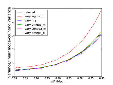
Since the different terms in the covariance matrix scale either like the second or third power of the power spectrum, we expect a significant dependence on and other parameters changing the overall normalization of the spectrum. The beat coupling/local average term is particularly sensitive to the power at so that it should depend on any parameter that affects the power on very large scales. To make this more quantitative, we consider the CDM fiducial cosmology described in section III and change each parameter by a step , one by one, keeping the remaining parameters fixed. For the step sizes, we choose , where is the parameter uncertainty from Reid et al. (2010) (Table 3), obtained from combining the SDSS-II Data Release 7 Abazajian et al. (2009) halo power spectrum with WMAP5 Dunkley et al. (2009) cosmic microwave background (CMB) data. These step sizes are indicative of the relevant parameter range in a Markov Chain Monte Carlo (MCMC) analysis with power spectrum data. We show the fiducial parameters and their step sizes in Table 1.
| fiducial | 0.023 | 0.1323 | 0.27 | 0.79 | 0.96 |
|---|---|---|---|---|---|
| step size | 0.00116 | 0.008 | 0.038 | 0.05 | 0.026 |
In the left panel of figure 10, we show the effect on the variance of each parameter. As before, we normalize the variance by the variance based on mode counting and the linear power spectrum (as calculated in the fiducial cosmology). The units on the horizontal axis are Mpc, where is the dimensionless Hubble parameter in the fiducial model. The variance in the fiducial model is given by the black curve. As expected, the largest variation is obtained when varying , causing a significant increase in variance. The effect of the other parameters is much smaller.
The effect of the parameter variations on the correlation coefficients is always below , with decreasing the coefficients most, and increasing them by the largest amount. Finally, to incorporate the properties of the full covariance matrix in a single statistic, we calculate the squared signal-to-noise ratio in the (non-linear) power spectrum amplitude as a function of , see Eq. (26). In a more thorough analysis, one could replace the power spectrum in the expression for by derivatives with respect to cosmological parameters in order to create a full Fisher matrix.
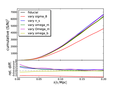
The right panel of figure 10 depicts this signal-to-noise squared as a function of for the different cosmologies, with the bottom inset showing the relative difference with respect to in the fiducial model. We focus on the range Mpc, as this is a more realistic range for a galaxy survey (due to strong non-linearities and shot noise on smaller scales), and because we have seen that our approach loses accuracy on smaller scales. Consistent with the picture arising from the left panel, we see again that has by far the largest effect, decreasing the signal-to-noise by (with only a weak dependence of the relative change on ). The other parameters have a much more modest effect ( for Mpc). We conclude that reasonable variations in cosmic parameters can cause changes in the covariance matrix and thus in values in an MCMC chain.
Finally, we note that, for a galaxy survey, the effect of galaxy bias on the covariance matrix will be very important as well, and will look similar to the effect of discussed above.
References
- Seo and Eisenstein (2003) H. Seo and D. J. Eisenstein, Astrophys. J. 598, 720 (2003), eprint arXiv:astro-ph/0307460.
- Eisenstein et al. (2005) D. J. Eisenstein, I. Zehavi, D. W. Hogg, R. Scoccimarro, M. R. Blanton, R. C. Nichol, R. Scranton, H.-J. Seo, M. Tegmark, Z. Zheng, et al., Astrophys. J. 633, 560 (2005), eprint arXiv:astro-ph/0501171.
- Cole et al. (2005) S. Cole, W. J. Percival, J. A. Peacock, P. Norberg, C. M. Baugh, C. S. Frenk, I. Baldry, J. Bland-Hawthorn, T. Bridges, R. Cannon, et al., Mon. Not. R. Astron. Soc. 362, 505 (2005), eprint arXiv:astro-ph/0501174.
- Blake et al. (2011) C. Blake, E. A. Kazin, F. Beutler, T. M. Davis, D. Parkinson, S. Brough, M. Colless, C. Contreras, W. Couch, S. Croom, et al., Mon. Not. R. Astron. Soc. p. 1598 (2011), eprint 1108.2635.
- Efstathiou et al. (2002) G. Efstathiou, S. Moody, J. A. Peacock, W. J. Percival, C. Baugh, J. Bland-Hawthorn, T. Bridges, R. Cannon, S. Cole, M. Colless, et al., Mon. Not. R. Astron. Soc. 330, L29 (2002), eprint arXiv:astro-ph/0109152.
- Reid et al. (2010) B. A. Reid, W. J. Percival, D. J. Eisenstein, L. Verde, D. N. Spergel, R. A. Skibba, N. A. Bahcall, T. Budavari, J. A. Frieman, M. Fukugita, et al., Mon. Not. R. Astron. Soc. 404, 60 (2010), eprint 0907.1659.
- Feldman et al. (1994) H. A. Feldman, N. Kaiser, and J. A. Peacock, Astrophys. J. 426, 23 (1994), eprint arXiv:astro-ph/9304022.
- Scoccimarro et al. (1999) R. Scoccimarro, M. Zaldarriaga, and L. Hui, Astrophys. J. 527, 1 (1999), eprint arXiv:astro-ph/9901099.
- Meiksin and White (1999) A. Meiksin and M. White, Mon. Not. R. Astron. Soc. 308, 1179 (1999), eprint arXiv:astro-ph/9812129.
- Cooray and Hu (2001) A. Cooray and W. Hu, Astrophys. J. 554, 56 (2001), eprint arXiv:astro-ph/0012087.
- Scoccimarro and Sheth (2002) R. Scoccimarro and R. K. Sheth, Mon. Not. R. Astron. Soc. 329, 629 (2002), eprint arXiv:astro-ph/0106120.
- Sirko (2005) E. Sirko, Astrophys. J. 634, 728 (2005), eprint arXiv:astro-ph/0503106.
- Sefusatti et al. (2006) E. Sefusatti, M. Crocce, S. Pueblas, and R. Scoccimarro, Phys. Rev. D 74, 023522 (2006), eprint arXiv:astro-ph/0604505.
- Neyrinck et al. (2006) M. C. Neyrinck, I. Szapudi, and C. D. Rimes, Mon. Not. R. Astron. Soc. 370, L66 (2006), eprint arXiv:astro-ph/0604282.
- Neyrinck and Szapudi (2007) M. C. Neyrinck and I. Szapudi, Mon. Not. R. Astron. Soc. 375, L51 (2007), eprint arXiv:astro-ph/0610211.
- Smith (2009) R. E. Smith, Mon. Not. R. Astron. Soc. 400, 851 (2009), eprint 0810.1960.
- Sato et al. (2009) M. Sato, T. Hamana, R. Takahashi, M. Takada, N. Yoshida, T. Matsubara, and N. Sugiyama, Astrophys. J. 701, 945 (2009), eprint 0906.2237.
- Neyrinck (2011) M. C. Neyrinck, Astrophys. J. 736, 8 (2011), eprint 1103.5476.
- Harnois-Deraps and Pen (2011) J. Harnois-Deraps and U.-L. Pen, ArXiv e-prints (2011), eprint 1109.5746.
- Ngan et al. (2011) W.-H. W. Ngan, J. Harnois-Déraps, U.-L. Pen, P. McDonald, and I. MacDonald, ArXiv e-prints (2011), eprint 1106.5548.
- Hamilton et al. (2006) A. J. S. Hamilton, C. D. Rimes, and R. Scoccimarro, Mon. Not. R. Astron. Soc. 371, 1188 (2006), eprint arXiv:astro-ph/0511416.
- Rimes and Hamilton (2006) C. D. Rimes and A. J. S. Hamilton, Mon. Not. R. Astron. Soc. 371, 1205 (2006), eprint arXiv:astro-ph/0511418.
- Takada and Jain (2009) M. Takada and B. Jain, Mon. Not. R. Astron. Soc. 395, 2065 (2009), eprint 0810.4170.
- Reid et al. (2009) B. A. Reid, D. N. Spergel, and P. Bode, Astrophys. J. 702, 249 (2009), eprint 0811.1025.
- Takahashi et al. (2009) R. Takahashi, N. Yoshida, M. Takada, T. Matsubara, N. Sugiyama, I. Kayo, A. J. Nishizawa, T. Nishimichi, S. Saito, and A. Taruya, Astrophys. J. 700, 479 (2009), eprint 0902.0371.
- Bernardeau et al. (2002) F. Bernardeau, S. Colombi, E. Gaztañaga, and R. Scoccimarro, Physics Reports 367, 1 (2002), eprint arXiv:astro-ph/0112551.
- Fry (1984) J. N. Fry, Astrophys. J. 279, 499 (1984).
- Goroff et al. (1986) M. H. Goroff, B. Grinstein, S.-J. Rey, and M. B. Wise, Astrophys. J. 311, 6 (1986).
- Neyrinck et al. (2009) M. C. Neyrinck, I. Szapudi, and A. S. Szalay, Astrophys. J. Lett. 698, L90 (2009), eprint 0903.4693.
- Smith et al. (2003) R. E. Smith, J. A. Peacock, A. Jenkins, S. D. M. White, C. S. Frenk, F. R. Pearce, P. A. Thomas, G. Efstathiou, and H. M. P. Couchman, Mon. Not. R. Astron. Soc. 341, 1311 (2003), eprint arXiv:astro-ph/0207664.
- Lewis et al. (2000) A. Lewis, A. Challinor, and A. Lasenby, Astrophys.J. 538, 473 (2000), eprint arXiv:astro-ph/9911177.
- Komatsu et al. (2010) E. Komatsu, K. M. Smith, J. Dunkley, C. L. Bennett, B. Gold, G. Hinshaw, N. Jarosik, D. Larson, M. R. Nolta, L. Page, et al., ArXiv e-prints (2010), eprint arXiv:1001.4538.
- Springel (2005) V. Springel, Mon. Not. R. Astron. Soc. 364, 1105 (2005), eprint arXiv:astro-ph/0505010.
- Jing (2005) Y. P. Jing, Astrophys. J. 620, 559 (2005), eprint arXiv:astro-ph/0409240.
- Tegmark et al. (2006) M. Tegmark, D. J. Eisenstein, M. A. Strauss, D. H. Weinberg, M. R. Blanton, J. A. Frieman, M. Fukugita, J. E. Gunn, A. J. S. Hamilton, G. R. Knapp, et al., Phys.Rev.D 74, 123507 (2006), eprint arXiv:astro-ph/0608632.
- Abazajian et al. (2009) K. N. Abazajian, J. K. Adelman-McCarthy, M. A. Agüeros, S. S. Allam, C. Allende Prieto, D. An, K. S. J. Anderson, S. F. Anderson, J. Annis, N. A. Bahcall, et al., Astrophys. J. Suppl. 182, 543 (2009), eprint 0812.0649.
- Dunkley et al. (2009) J. Dunkley, E. Komatsu, M. R. Nolta, D. N. Spergel, D. Larson, G. Hinshaw, L. Page, C. L. Bennett, B. Gold, N. Jarosik, et al., Astrophys. J. Suppl. 180, 306 (2009), eprint 0803.0586.