Dimensions of attractors in pinched skew products

Abstract

We study dimensions of strange non-chaotic attractors and their associated physical measures in so-called pinched skew products, introduced by Grebogi and his coworkers in 1984. Our main results are that the Hausdorff dimension, the pointwise dimension and the information dimension are all equal to one, although the box-counting dimension is known to be two. The assertion concerning the pointwise dimension is deduced from the stronger result that the physical measure is rectifiable. Our findings confirm a conjecture by Ding, Grebogi and Ott from 1989.

1 Introduction

In [1], Grebogi and coworkers introduced (a slight variation of) the system

(1.1) $$F_{\kappa}\ :\ \mathbb{T}^{1}\times[0,1]\to\mathbb{T}^{1}\times[0,1]\quad,\quad F_{\kappa}(\theta,x)\ =\ (\theta+\rho\bmod 1,\tanh(\kappa x)\cdot\sin(\pi\theta))\ ,$$

with $\rho\in\mathbb{R}\setminus\mathbb{Q}$ and real parameter $\kappa>0$, as a simple model for the existence of strange non-chaotic attractors (SNA). Later, the term ‘pinched skew products’ was coined by Glendinning [2] for a general class of systems sharing some essential properties of (1.1). The object which is called an SNA in the above system is the upper bounding graph $\varphi^{+}$ of the global attractor $\mathcal{A}:=\bigcap_{n\in\mathbb{N}}F_{\kappa}^{n}(\mathbb{T}^{1}\times[0,1])$, which is given by

(1.2) $$\varphi^{+}(\theta)\ :=\ \sup\{x\in[0,1]\mid(\theta,x)\in\mathcal{A}\}\ .$$

An illustration of this attractor is shown in Figure 1.1.

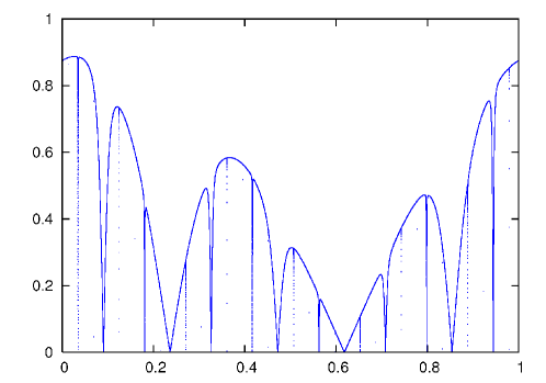
Figure 1.1: Strange non-chaotic attractor in (1.2) with $\kappa=3$ and $\rho$ the golden mean.

Due to the monotonicity of the fibre maps $F_{\kappa,\theta}:x\mapsto\tanh(\kappa x)\cdot\sin(\pi\theta)$, one can verify that the function $\varphi^{+}$ satisfies

(1.3) $$F_{\kappa,\theta}(\varphi^{+}(\theta))\ =\ \varphi^{+}(\theta+\rho\bmod 1)\ .$$

Consequently, the corresponding point set $\Phi^{+}:=\{(\theta,\varphi^{+}(\theta))\mid\theta\in\mathbb{T}^{1}\}$ is $F_{\kappa}$-invariant. Slightly abusing terminology, we will call both $\varphi^{+}$ and $\Phi^{+}$ an invariant graph. Keller showed in [3] that for $\kappa>2$ in (1.1) the graph $\varphi^{+}$ is $\mathrm{Leb}_{\mathbb{T}^{1}}$-almost surely strictly positive, its Lyapunov exponent

$$\lambda(\varphi^{+})\ =\ \int\log F_{\kappa,\theta}^{\prime}(\varphi^{+}(\theta))\ d\theta$$

is strictly negative and $\varphi^{+}$ attracts $\mathrm{Leb}_{\mathbb{T}^{1}\times[0,1]}$-a.e. initial condition. Note that Birkhoff’s Ergodic Theorem implies that $\lim_{n\rightarrow\infty}\frac{1}{n}\log\left(F_{\kappa,\theta}^{n}\right)^{\prime}(\varphi^{+}(\theta))=\lambda(\varphi^{+})$ for $\mathrm{Leb}_{\mathbb{T}^{1}}$-a.e. $\theta\in\mathbb{T}^{1}$, where we let $F^{n}_{\kappa,\theta}=F_{\kappa,\theta+(n-1)\rho\bmod 1}\circ\ldots\circ F_{\kappa,\theta}$.

The findings in [1] attracted substantial interest in the theoretical physics community, and subsequently a large number of numerical studies confirmed the widespread existence of SNA in quasiperiodically forced systems and explored their behaviour and properties (see [4, 5, 6] for an overview and further references). For a long time, however, rigorous results remained rare, and even basic questions are still open nowadays. In particular, this concerns the dimensions and fractal properties of SNA, which are still mostly unknown even for the original example by Grebogi et al. A numerical investigation was carried out in [7], and the results indicated that the box dimension of the attractor is two, whereas the information dimension should be one. For sufficiently large $\kappa$, the conjecture on the box dimension was verified indirectly in [8], by showing that the topological closure of $\Phi^{+}$ is equal to the global attractor $\mathcal{A}=\{(\theta,x)\mid 0\leq x\leq\varphi^{+}(\theta)\}$ and therefore has positive two dimensional Lebesgue measure.

Our aim is to determine further dimensions of $\varphi^{+}$ and the associated invariant measure $\mu_{\varphi^{+}}$, which is obtained by projecting the Lebesgue measure on the base $\mathbb{T}^{1}$ onto $\Phi^{+}$. For the Hausdorff dimension $D_{H}$ (see Section 2.2 for the definition), we have

Theorem 1.1.

Suppose $\rho$ in (1.1) is Diophantine and $\kappa$ is sufficiently large. Then $D_{H}(\Phi^{+})=1$. Furthermore, the one-dimensional Hausdorff measure of $\Phi^{+}$ is infinite.

This statement is a special case of Corollary 5.6, see Section 5. Here and in the results below, the largness condition of $\kappa$ depends on the constants of the Diophantine condition on $\rho$.

Remark 1.2.

Our results in Section 5 also allow to treat examples with a higher dimensional driving space, as given in Example 4.1. In these cases, the rotation on $\mathbb{T}^{1}$ is replaced by a rotation on $\mathbb{T}^{D}$, and we obtain that the Hausdorff dimension of $\Phi^{+}$ is $D$. However, at least for sufficiently large $D$ the $D$-dimensional Hausdorff measure is finite, in contrast to the case $D=1$ (Proposition 5.3). We believe that for these examples the $D$-dimensional Hausdorff measure is infinite only for $D=1$ and finite for all $D\geq 2$.

In order to obtain information on the invariant measure $\mu_{\varphi^{+}}$, we determine its pointwise dimension given by

$$d_{\mu_{\varphi^{+}}}(\theta,x)\ =\ \lim_{\varepsilon\to 0}\frac{\log\mu_{\varphi^{+}}(B_{\varepsilon}(\theta,x))}{\log\varepsilon}.$$

A priori, it is not clear whether this limit exists, such that in general one defines the upper and lower pointwise dimension by taking the limit superior and inferior, respectively (see Section 2.2). Furthermore, even if the limit exists, it may depend on $(\theta,x)$. If the pointwise dimension exists and is constant almost surely, the invariant measure is called exact dimensional. It turns out that this is the case in the situation considered here. In fact, we obtain the stronger result that $\mu_{\varphi^{+}}$ is a rectifiabile measure, see Section 2.3 and Theorem 5.5, and this directly implies

Theorem 1.3.

Suppose $\rho$ in (1.1) is Diophantine and $\kappa$ is sufficiently large. Then for $\mu_{\varphi^{+}}$-almost every $(\theta,x)\in\mathbb{T}^{1}\times[0,1]$, we have $d_{\mu_{\varphi^{+}}}(\theta,x)=1$. In particular, $\mu_{\varphi^{+}}$ is exact dimensional.

For an exact dimensional measure $\mu$, it is known that the information dimension $D_{1}$ (see again Section 2.2 for the definition) coincides with the pointwise dimension. Hence, we obtain

Corollary 1.4.

Suppose $\rho$ in (1.1) is Diophantine and $\kappa$ is sufficiently large. Then $D_{1}(\mu_{\varphi^{+}})=1$.

This confirms the conjecture made in [7]. Since the geometric mechanism for the creation of SNA in pinched skew products is quite universal and can be found in similar form in other types of systems, we expect our results to hold in further situations. For example, this should be true for the SNA found in the Harper map, which describes the projective action of quasiperiodic Schrödinger cocycles, and for SNA in the quasiperiodically forced versions of the logistic map and the Arnold circle map. On a technical level, these systems are much more difficult to deal with, and for this reason we refrain from extending our analysis beyond pinched skew products here. Yet, combining our approach with the methods developed in [9, 10, 14] should allow to produce similar results for the mentioned examples. Apart from this, progress has also been made recently concerning the existence of SNA in quasiperiodically forced unimodal maps [11, 12, 13] . Here, similar results may be expected as well, but it is much less clear to what extend the presented techniques can be adapted.

Our proof hinges on the fact that the SNA $\varphi^{+}$ can be approximated by the iterates of the upper bounding line $\mathbb{T}^{1}\times\{1\}$ of the phase space, whose geometry can be controlled quite accurately. This observation has already been used in [8] and will be exploited further here. An outline of the strategy is given in Section 3. In Section 4 we derive the required estimates on the approximating curves, which are used to compute the Hausdorff dimension and the pointwise dimension in Section 5.

Acknowledgments. This work was supported by an Emmy-Noether-Grant of the German Research Council (DFG grant JA 1721/2-1) and is part of the activities of the Scientific Network “Skew product dynamics and multifractal analysis” (DFG grant OE 538/3-1). We thank René Schilling for his thoughtful comment leading to Proposition 5.7.

2 Preliminaries

2.1 Strange non-chaotic attractors

In the following, we provide some basics on SNA in pinched skew products by sketching Keller’s proof for the existence of SNA [3]. More precisely, according to [1] the upper bounding graph $\varphi^{+}$ is called an SNA if it is non-continuous and has a negative Lyapunov exponent, and we will mainly explain how to obtain the non-continuity.

Let $I=[0,1]$ and $\mathbb{T}^{D}=\mathbb{R}^{D}/\mathbb{Z}^{D}$. A quasiperiodically forced interval map is a skew product map of the form

$$T\ :\ \mathbb{T}^{D}\times I\to\mathbb{T}^{D}\times I\quad,\quad(\theta,x)\mapsto(\omega(\theta),T_{\theta}(x))\ ,$$

where $\omega:\mathbb{T}^{D}\to\mathbb{T}^{D},\ \theta\mapsto\theta+\rho\bmod 1$ an irrational rotation. The maps $T_{\theta}:I\to I$ are called fibre maps. $T$ is pinched if there exists some $\theta_{*}\in\mathbb{T}^{D}$ with $\#T_{\theta_{*}}(I)=1$.

We denote by $\mathcal{T}$ the class of quasiperiodically forced interval maps $T$ which share the following properties:

• the fibre maps $T_{\theta}$ are monotonically increasing;

• the fibre maps $T_{\theta}$ are differentiable and $(\theta,x)\mapsto T_{\theta}^{\prime}(x)$ is continuous on $\mathbb{T}^{D}\times I$;

• $T$ is pinched;

• $T_{\theta}(0)=0$ for all $\theta\in\mathbb{T}^{D}$.

Note that the last item means that the zero line $\mathbb{T}^{D}\times\{0\}$ is $T$-invariant. It is easy to check that the maps $F_{\kappa}$ defined in (1.1) belong to $\mathcal{T}$.

An invariant graph is a measurable function $\varphi:\mathbb{T}^{D}\to I$ which satisfies (1.3). If all fibre maps are differentiable, the Lyapunov exponent of $\varphi$ is given by $\lambda(\varphi):=\int_{\mathbb{T}^{D}}\log T_{\theta}^{\prime}(\varphi(\theta))\ d\theta$. The upper bounding graph $\varphi^{+}$ is given by (1.2). Equivalently, it can be defined by

$$\varphi^{+}(\theta)\ =\ \lim_{n\rightarrow\infty}T^{n}_{\omega^{-n}(\theta)}(1),$$

where $T^{n}_{\theta}=T_{\omega^{n-1}(\theta)}\circ\ldots\circ T_{\theta}$. This means that the iterated upper bounding lines

(2.1) $$\varphi_{n}(\theta)\ :=\ T^{n}_{\omega^{-n}(\theta)}(1)$$

converge pointwise and, by monotonicity of the fibre maps, in a decreasing way to $\varphi^{+}$. This fact will be crucial for our later analysis. A first consequence of this observation is that, under some mild conditions, the Lyapunov exponent of $\varphi^{+}$ is always non-positive.

Lemma 2.1 ([15, Lemma 3.5]).

If $\theta\mapsto\log\left(\inf_{x\in I}T^{\prime}_{\theta}(x)\right)$ is integrable, then $\lambda(\varphi^{+})\leq 0$.

Now, turning back to the maps $F_{\kappa}$ defined in (1.1), the Lyapunov exponent of the zero line is easily computed and one obtains

$$\lambda(0)\ =\ \log\kappa-\log 2.$$

Consequently, when $\kappa>2$ this exponent is positive and therefore the upper bounding graph cannot be the zero line. However, at the same time the pinching condition together with the invariance of $\varphi^{+}$ imply that $\varphi^{+}(\theta)=0$ for a dense set of $\theta\in\mathbb{T}^{1}$. Hence, $\varphi^{+}$ cannot be continuous.

Using the concavity of the fibre maps, it is further possible to show that $\varphi^{+}$ is the only invariant graph of the system (1.1) besides the zero line, that $\lambda(\varphi^{+})$ is strictly negative and that $\varphi^{+}$ attracts $\mathrm{Leb}_{\mathbb{T}^{1}\times I}$-a.e. initial condition $(\theta,x)$, in the sense that

$$\lim_{n\rightarrow\infty}F_{\kappa,\theta}^{n}(x)-\varphi^{+}(\theta+n\rho\bmod 1)\ =\ 0.$$

Finally, we note that to any invariant graph $\varphi$, an invariant measure $\mu_{\varphi}$ can be associated by

$$\mu_{\varphi}(A)\ :=\ \mathrm{Leb}_{\mathbb{T}^{D}}(\pi_{1}(A\cap\Phi))$$

for all Borel measurable sets $A\subseteq\mathbb{T}^{D}\times I$, where $\pi_{1}:\mathbb{T}^{D}\times I\to\mathbb{T}^{D}$ is the projection to the first coordinate.

2.2 Dimensions

Let $X$ be a separable metric space. The diameter of a subset $A\subseteq X$ is denoted by $\mathrm{diam}(A)$. For $\varepsilon>0$ a finite or countable collection $\{A_{i}\}$ of subsets of $X$ is called an $\varepsilon$-cover of $A$ if $\mathrm{diam}(A_{i})\leq\varepsilon$ for each $i$ and $A\subseteq\bigcup_{i}A_{i}$.

Definition 2.2.

For $A\subseteq X$, $s\geq 0$ and $\varepsilon>0$ define

$$\mathcal{H}_{\varepsilon}^{s}(A)\ :=\ \inf\left\{\left.\sum\limits_{i}(\mathrm{diam}(A_{i}))^{s}\ \right|\ \{A_{i}\}\text{ is an $\varepsilon$-cover of $A$}\right\}.$$

Then

$$\mathcal{H}^{s}(A)\ :=\ \lim\limits_{\varepsilon\to 0}\mathcal{H}_{\varepsilon}^{s}(A)$$

is called the $s$-dimensional Hausdorff measure of $A$. The Hausdorff dimension of $A$ is defined by

$$D_{H}(A)\ :=\ \sup\{s\geq 0\mid\mathcal{H}^{s}(A)=\infty\}.$$

Definition 2.3.

The lower and upper box-counting dimension of a totally bounded subset $A\subseteq X$ are defined as

$$\underline{D}_{B}(A)\ :=\ \liminf\limits_{\varepsilon\to 0}\frac{\log N(A,\varepsilon)}{-\log\varepsilon},$$

$$\overline{D}_{B}(A)\ :=\ \limsup\limits_{\varepsilon\to 0}\frac{\log N(A,\varepsilon)}{-\log\varepsilon},$$

where $N(A,\varepsilon)$ is the smallest number of sets of diameter $\varepsilon$ needed to cover $A$. If $\underline{D}_{B}(A)=\overline{D}_{B}(A)$, then their common value $D_{B}(A)$ is called the box-counting dimension (or capacity) of $A$.

In general, we have $D_{H}(A)\leq D_{B}(A)$. In the following, we will state some well known properties of the Hausdorff measure and dimension that will be used later on.

Lemma 2.4 ([16]).

Let $X,Y$ be two separable metric spaces and let $g:A\subseteq X\to Y$ be a Lipschitz continuous map with Lipschitz constant $K$. Then $\mathcal{H}^{s}(g(A))\leq K^{s}\mathcal{H}^{s}(A)$ and $D_{H}(g(A))\leq D_{H}(A)$. Further, if $g$ is bi-Lipschitz continuous, then $D_{H}(g(A))=D_{H}(A)$.

Lemma 2.5 ([16]).

The Hausdorff dimension is countably stable, i.e. $D_{H}\left(\bigcup_{i}A_{i}\right)=\sup_{i}D_{H}(A_{i})$ for any sequence of subsets $(A_{i})_{i\in\mathbb{N}}$ with $A_{i}\subseteq X$ .

In contrast to the last lemma, we have that the upper box-counting dimension is only finitely stable and that $D_{B}(A)=D_{B}\left(\overline{A}\right)$.

Theorem 2.6 ([17]).

Let $X,Y$ be two separable metric spaces and consider the Cartesian product space $X\times Y$ equipped with the maximum metric. Then for $A\subseteq X$ and $B\subseteq Y$ totally bounded we have

$$D_{H}(A\times B)\ \leq\ D_{H}(A)+\overline{D}_{B}(B).$$

Lemma 2.7.

Let $A\subseteq X$ be a $\limsup$ set, meaning that there exists a sequence $(A_{i})_{i\in\mathbb{N}}$ of subsets of $X$ with

$$A\ =\ \limsup\limits_{i\to\infty}A_{i}\ =\ \bigcap\limits_{i=0}^{\infty}\bigcup\limits_{k=i+1}^{\infty}A_{k}.$$

If $\sum_{i=1}^{\infty}\mathrm{diam}(A_{i})^{s}<\infty$ for some $s>0$, then $\mathcal{H}^{s}(A)=0$ and $D_{H}(A)\leq s$.

Proof.

Since $\sum_{i=1}^{\infty}\mathrm{diam}(A_{i})^{s}<\infty$, we have $\sum_{i=k}^{\infty}\mathrm{diam}(A_{i})^{s}\to 0$ for $k\to\infty$. That means the diameter of the $A_{i}$’s goes to $0$ for $i\to\infty$. Therefore, $\{A_{i}:i\geq k\}$ is an $\varepsilon$-cover for $k$ sufficiently large. This implies $\mathcal{H}_{\varepsilon}^{s}(A)\leq\sum_{i=k}^{\infty}\mathrm{diam}(A_{i})^{s}\to 0$ for $k\to\infty$. Hence, $\mathcal{H}^{s}(A)=0$ and $D_{H}(A)\leq s$. ∎

For $x\in X$ and $\varepsilon>0$ we denote by $B_{\varepsilon}(x)$ the open ball around $x$ with radius $\varepsilon>0$.

Definition 2.8.

Let $\mu$ be a finite Borel measure in $X$. For each point $x$ in the support of $\mu$ we define the lower and upper pointwise dimension of $\mu$ at $x$ as

$$\underline{d}_{\mu}(x)\ :=\ \liminf\limits_{\varepsilon\to 0}\frac{\log\mu(B_{\varepsilon}(x))}{\log\varepsilon},$$

$$\overline{d}_{\mu}(x)\ :=\ \limsup\limits_{\varepsilon\to 0}\frac{\log\mu(B_{\varepsilon}(x))}{\log\varepsilon}.$$

If $\underline{d}_{\mu}(x)=\overline{d}_{\mu}(x)$, then their common value $d_{\mu}(x)$ is called the pointwise dimension of $\mu$ at $x$. We say that the measure $\mu$ is exact dimensional if the pointwise dimension exists and is constant almost everywhere, i.e.

$$\underline{d}_{\mu}(x)\ =\ \overline{d}_{\mu}(x)\ =:\ d_{\mu},$$

$\mu$-almost everywhere.

Definition 2.9.

The lower and upper information dimension of $\mu$ are defined as

$$\underline{D}_{1}(\mu):=\liminf\limits_{\varepsilon\to 0}\frac{\int\log\mu(B_{\varepsilon}(x))d\mu(x)}{\log\varepsilon},$$

$$\overline{D}_{1}(\mu):=\limsup\limits_{\varepsilon\to 0}\frac{\int\log\mu(B_{\varepsilon}(x))d\mu(x)}{\log\varepsilon}.$$

If $\underline{D}_{1}(\mu)=\overline{D}_{1}(\mu)$, then their common value $D_{1}(\mu)$ is called the information dimension of $\mu$.

Theorem 2.10 ([18, 20]).

Suppose $\overline{D}_{B}(X)<\infty$. We have

$$\int\underline{d}_{\mu}(x)\ d\mu(x)\ \leq\ \underline{D}_{1}(\mu)\ \leq\ \overline{D}_{1}(\mu)\ \leq\ \int\overline{d}_{\mu}(x)\ d\mu(x).$$

In particular, if $\mu$ is exact dimensional, then $D_{1}(\mu)=d_{\mu}$.

Note that also several other dimensions of $\mu$ coincide if $\mu$ is exact dimensional [19, 20, 21, 22].

2.3 Rectifiable sets and measures

Here, we mainly follow [23].

Definition 2.11.

For $D\in\mathbb{N}$ a Borel set $A\subseteq X$ is called countably $D$-rectifiable if there exists a sequence of Lipschitz continuous functions $(g_{i})_{i\in\mathbb{N}}$ with $g_{i}:A_{i}\subseteq\mathbb{R}^{D}\to X$ such that $\mathcal{H}^{D}(A\backslash\bigcup_{i}g_{i}(A_{i}))=0$. A finite Borel measure $\mu$ is called $D$-rectifiable if $\mu=\Theta\left.\mathcal{H}^{D}\right|_{A}$ for some countably $D$-rectifiable set $A$ and some Borel measurable density $\Theta:A\to[0,\infty)$.

Note that, by the Radon-Nikodym theorem, $\mu$ is $D$-rectifiable if and only if $\mu$ is absolutely continuous with respect to $\left.\mathcal{H}^{D}\right|_{A}$ with $A$ some countably $D$-rectifiable set.

Theorem 2.12 ([23, Theorem 5.4]).

For a $D$-rectifiable measure $\mu=\Theta\left.\mathcal{H}^{D}\right|_{A}$ we have

$$\Theta(x)\ =\ \lim\limits_{\varepsilon\to 0}\frac{\mu(B_{\varepsilon}(x))}{V_{D}\varepsilon^{D}},$$

for $\mathcal{H}^{D}$-a.e. $x\in A$, where $V_{D}$ is the volume of the $D$-dimensional unit ball. The right hand side of this equation is called $D$-density of $\mu$.

This theorem implies in particular that the $D$-density exists and is positive $\mu$-almost everywhere for a $D$-rectifiable measure $\mu$ and this gives directly

Corollary 2.13.

A $D$-rectifiable measure $\mu$ is exact dimensional with $d_{\mu}=D_{1}(\mu)=D$.

3 Outline of the strategy

As we have mentioned in the introduction, our main goal is to analyze the structure of the upper bounding graphs $\varphi^{+}$ when they are different from the zero line, and in particular we want to determine the dimensions of these graphs and of their associated invariant measures. However, the argument for the non-continuity of the invariant graphs sketched in Section 2.1 is a ‘soft’ one and does not yield any quantitative information about the structure of the invariant graphs. Hence, it is not clear how such an analysis can be carried out.

However, as mentioned above the upper bounding graph $\varphi^{+}$ can be approximated by the iterated upper bounding lines $\varphi_{n}$ defined in (2.1). It turns out that the geometry of the lines $\varphi_{n}$ can be controlled well, and this is the starting point of our investigation. Figure 3.1 shows the first six iterates $\varphi_{1},\ldots,\varphi_{6}$. A clear pattern can be observed. Apparently, when going from $\varphi_{n-1}$ to $\varphi_{n}$, the only significant change is the appearance of a new ‘peak’ in a small ball $I_{n}$ around the $n$-th iterate $\tau_{n}=\omega^{n}(\theta_{*})$ of the pinching point $\theta_{*}$. Outside of $I_{n}$, the graphs seem to remain unchanged. Further, since every new peak is the image of the previous one and due to the expansion around the 0-line, the peaks become steeper and sharper in every step. As a consequence, the radius of the balls $I_{n}$ decreases exponentially.

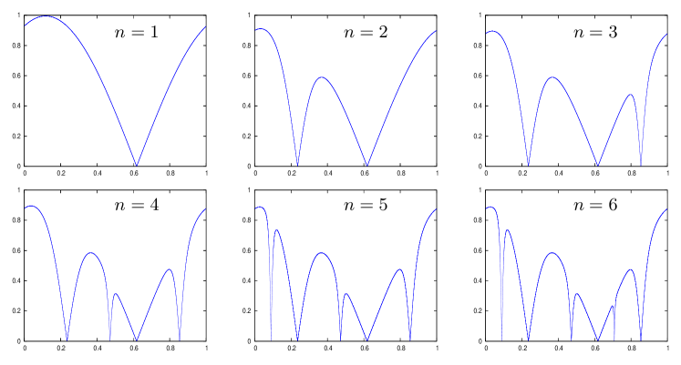
Figure 3.1: The graphs of the first six iterated upper bounding lines of (1.1) with $\kappa=3$ and $\rho$ the golden mean.

Of course, this is a very rough picture, which can only hold in an approximate sense. Due to the strict monotonicity of the fibre maps for all $\theta\neq\theta_{*}$, the sequence $\varphi_{n}$ is strictly decreasing everywhere except on the countable set $\{\tau_{n}\mid n\in\mathbb{N}\}$, so the graphs have to change at least a little bit outside of $I_{n}$. However, let us assume for the moment that the above description was true and $\varphi_{n-1}(\theta)-\varphi_{n}(\theta)=0$ for all $\theta\notin I_{n}$. In this case, the graph $\varphi^{+}$ is already determined on $\mathbb{T}^{D}\setminus\bigcup_{k=n}^{\infty}I_{k}=:\Lambda_{n}$ after $n$ steps and equals $\varphi_{n|\Lambda_{n}}$ on this set. However, as a finite iterate of $\mathbb{T}^{D}\times\{1\}$, the function $\varphi_{n}$ is Lipschitz continuous and therefore its graph $\Phi_{n|\Lambda_{n}}=\{(\theta,\varphi_{n}(\theta))\mid\theta\in\Lambda_{n}\}$ has Hausdorff dimension $D$. Due to the exponential decrease of the radius of the $I_{n}$, the set $\Omega_{\infty}=\mathbb{T}^{D}\setminus\bigcup_{n\in\mathbb{N}}\Lambda_{n}$ is a $\limsup$ set and has Hausdorff dimension zero by Lemma 2.7. It follows that $\Phi^{+}$ is contained in the countable union $\bigcup_{n\in\mathbb{N}}\Phi_{n|\Lambda_{n}}\cup(\Omega_{\infty}\times[0,1])$ of at most D-dimensional sets. By countable stability, this implies that the Hausdorff dimension of $\Phi^{+}$ is $D$. For the pointwise dimension, a similar argument could be given but we will directly conclude from the arguments sketched above that $\mu_{\varphi^{+}}$ is $D$-rectifiable.

The remainder of this article is devoted to showing that these heuristics can be converted into a rigorous proof, despite the fact that ‘nothing changes outside of $I_{n}$’ has to be replaced by ‘almost nothing changes outside of $I_{n}$’.

4 Estimates on the iterated upper bounding lines

The purpose of this section is to obtain a good control on the behaviour and shape of the iterated upper bounding lines. In order to derive the required estimates, we have to impose a number of assumptions on the geometry of our systems. The hypotheses are formulated in terms of ${\cal C}^{1}$-estimates, and it is easy to check that they are fulfilled by (1.1) whenever $\kappa$ is large enough (see Lemma 4.2 for details).

Let $T\in\mathcal{T}$. Suppose there exist $\alpha>2,\ \gamma>0$ and $L_{0}\in(0,1)$ such that for all $\theta\in\mathbb{T}^{D}$

(4.1) $$\left|T_{\theta}(x)-T_{\theta}(y)\right|\ \leq\ \alpha\left|x-y\right|,$$

for all $x,y\in[0,1]$, and

(4.2) $$\left|T_{\theta}(x)-T_{\theta}(y)\right|\ \leq\ \alpha^{-\gamma}\left|x-y\right|,$$

for all $x,y\in[L_{0},1]$. Further, we assume there exists $\beta>0$ such that for all $x\in[0,1]$

(4.3) $$\left|T_{\theta}(x)-T_{\theta^{\prime}}(x)\right|\ \leq\ \beta d(\theta,\theta^{\prime}).$$

When $T$ is differentiable in $\theta$, we may for example take $\beta=\sup_{(\theta,x)}\left\|\partial_{\theta}T_{\theta}(x)\right\|$. As above, we let $\tau_{n}:=\omega^{n}(\theta_{*})$. We suppose the rotation vector $\rho\in\mathbb{R}^{D}$ is Diophantine, meaning that there exist constants $c>0$ and $d>1$ such that

(4.4) $$d(\tau_{n},\theta_{*})\ \geq\ c\cdot n^{-d},$$

for all $n\in\mathbb{N}$. In addition, we assume there are $m\in\mathbb{N}$, $a>1$ and $0<b<1$ with

(4.5) $$m >\ 22\left(1+\frac{1}{\gamma}\right),$$

(4.6) $$a \ \geq\ (m+1)^{d},$$

(4.7) $$b \ \leq\ c,$$

(4.8) $$d(\tau_{n},\theta_{*}) \ >\ b\quad\textnormal{ for all }n\in\{1,\dots,m-1\}$$

such that

(4.9) $$T_{\theta}(x) \ \geq\ \min\{L_{0},ax\}\cdot\min\left\{1,\frac{2}{b}d(\theta,\theta_{*})\right\},$$

for all $(\theta,x)\in\mathbb{T}^{D}\times[0,1]$. We now let

(4.10) $$\mathcal{T}^{*}\ :=\ \left\{T\in\mathcal{T}\mid T\textrm{ satisfies (\ref{Lipschitz-fibres})--(\ref{definition_reference_system})}\right\}\ ,$$

where “satisfies (4.1)–(4.9)” should be understood in the sense of “there exist constants $\alpha$, $\gamma$, $L_{0}$, $\beta$, $c$, $d$, $m$, $a$ and $b$ such that (4.1)–(4.9) are satisfied”.

Example 4.1.

The following map is a simple extension of (1.1) with a higher-dimensional rotation on the base.

(4.11) $$F_{\kappa}\ :\ \mathbb{T}^{D}\times[0,1]\to\mathbb{T}^{D}\times[0,1]\quad,\quad F_{\kappa}(\theta,x)\ =\ \left(\theta+\rho\bmod 1,\tanh\left(\kappa x\right)\cdot\frac{1}{D}\cdot\sum\limits_{i=1}^{D}\sin(\pi\theta_{i})\right)$$

Here $\theta=(\theta_{1},\dots,\theta_{D})$.

As we show now, $F_{\kappa}$ satisfies (4.1) – (4.9) for all sufficiently large $\kappa$.

Lemma 4.2.

Let $\rho$ satisfy the Diophantine condition (4.4) with constants $c,d$. Then there exist constants $D_{0}=D_{0}(c,d)$ and $\kappa_{0}=\kappa_{0}(c,d,D)$ such that

• for all $\kappa\geq\kappa_{0}$ the map $F_{\kappa}$ belongs to $\mathcal{T}^{*}$;

• if $D\geq D_{0}$, then the constants $\alpha$, $m$ and $a$ can be chosen such that

  (4.12) $$D\ >\ m^{2}\log(\alpha/a)\ .$$

The additional condition (4.12) will be used to show that for sufficiently large $D$ the $D$-dimensional Hausdorff measure of the upper bounding graph $\varphi^{+}$ of $F_{\kappa}$ is finite, see Proposition 5.3.

Proof.

We let $\alpha=\kappa$, $\gamma=\frac{1}{2}$, $L_{0}=\frac{\log\kappa}{\kappa}$, $\beta=\pi$, $m=67$, $b=\frac{1}{2}\min_{n=1}^{m-1}cn^{-d}$ and $a=\frac{2b\kappa}{D(e+1/e)^{2}}$. Then we choose $D_{0}=D_{0}(c,d)$ such that for all $D\geq D_{0}$

(4.13) $$D\ >\ m^{2}\log\left(\frac{D(e+1/e)^{2}}{2b}\right)$$

and $\kappa_{0}=\kappa_{0}(c,d,D)$ such that for all $\kappa\geq\kappa_{0}$

(4.14) $$\kappa \geq 16\ ,$$

(4.15) $$\frac{2b\kappa}{D(e+1/e)^{2}} \geq (m+1)^{d}\ ,$$

(4.16) $$\frac{\log\kappa}{\kappa} \leq \frac{b\tanh(1)}{2D}\ .$$

We have

(4.17) $$\left[\tanh(\kappa x)\right]^{\prime}\ =\ \frac{4\kappa}{(e^{\kappa x}+e^{-\kappa x})^{2}}\ \leq\ \kappa$$

for all $x\geq 0$ and

(4.18) $$0\ \leq\ \frac{1}{D}\sum_{i=1}^{D}\sin(\pi\theta_{i})\ \leq\ 1$$

for all $\theta\in\mathbb{T}^{D}$. Hence, (4.1) holds and since

(4.19) $$F^{\prime}_{\kappa,\theta}(x)\ \leq\ F^{\prime}_{\kappa,\theta}(L_{0})\ \leq\ \frac{4\kappa}{(\kappa+1/\kappa)^{2}}\ \leq\ \frac{4}{\kappa}\ \leq\ \kappa^{-1/2}$$

for all $x\geq L_{0}$, the same is true for (4.2). (4.3) and (4.5) are easy to check, and (4.4) holds by assumption. (4.6) follows from (4.15), whereas (4.7) and (4.8) are obvious from the choice of $b$ and (4.4). In order to verify (4.9), note that $[\tanh(\kappa x)]^{\prime}_{|x=1/\kappa}=\frac{4\kappa}{(e+1/e)^{2}}$, such that by concavity and monotonicity

(4.20) $$\tanh(\kappa x)\ \geq\ \left\{\begin{array}[]{ll}\frac{4\kappa}{(e+1/e)^{2}}\cdot x&\textrm{if }x\leq 1/\kappa\\ \\ \tanh(1)&\textrm{if }x>1/\kappa\end{array}\right.\ .$$

Using (4.16) and the fact that $\sum_{i=1}^{D}\sin(\pi\theta_{i})\geq d(\theta,\theta_{*})$, where $\theta_{*}=0$, we obtain

$$F_{\kappa,\theta}(x) \geq \min\left\{\tanh(1),\frac{4\kappa}{(e+1/e)^{2}}x\right\}\cdot\frac{1}{D}d(\theta,\theta_{*})$$

$$\geq \min\left\{\frac{b\tanh(1)}{2D},\frac{2b\kappa}{D(e+1/e)^{2}}x\right\}\cdot\frac{2}{b}d(\theta,\theta_{*})$$

$$\geq \min\{L_{0},ax\}\cdot\min\left\{1,\frac{2}{b}d(\theta,\theta_{*})\right\}\$$

as required. Finally, since $\alpha/a=\frac{D(e+1/e)^{2}}{2b}$ condition (4.12) follows from (4.13). Note that since $b$ and $m$ are constants only depending on $c$ and $d$, the same is true for the condition (4.13) on $D_{0}$. ∎

Remark 4.3.

Given $T\in\mathcal{T}^{*}$, note that (4.9) implies

$$\lambda(0)\ \geq\ \log\frac{2a}{b}+\int_{\mathbb{T}^{D}}\log d(\theta,\theta_{*})\ d\theta\ \geq\ \log\frac{2a}{b}-\log 2-1\ .$$

Since $a\geq 23$ by (4.6), this yields $\lambda(0)>0$ and hence $\varphi^{+}(\theta)>0$ for $\mathrm{Leb}_{\mathbb{T}^{D}}$-almost every $\theta$.

In order to formulate the main results of this section, let $j\in\mathbb{R}$ and

$$r_{j}\ :=\ \frac{b}{2}a^{-\frac{j-1}{m}}\ .$$

Proposition 4.4.

Let $T\in\mathcal{T}^{*}$. Given $q\in\mathbb{N}$, the following hold.

1. $|\varphi_{n}(\theta)-\varphi_{n}(\theta^{\prime})|\leq\beta\alpha^{n}d(\theta,\theta^{\prime})$ for all $n\in\mathbb{N}$ and $\theta,\theta^{\prime}\in\mathbb{T}^{D}$.

2. There exists $\lambda>0$ such that if $n\geq mq+1$ and $\theta\notin\bigcup_{j=q}^{n}B_{r_{j}}(\tau_{j})$, then $|\varphi_{n}(\theta)-\varphi_{n-1}(\theta)|\leq\alpha^{-\lambda(n-1)}$.

3. There exists $K>0$ such that if $\theta,\theta^{\prime}\notin\bigcup_{j=q}^{n}B_{r_{j}}(\tau_{j})$, then $|\varphi_{n}(\theta)-\varphi_{n}(\theta^{\prime})|\leq K\alpha^{mq}d(\theta,\theta^{\prime})$ for all $n\in\mathbb{N}$.

For the proof, we need two preliminary statements. The first is a simple observation.

Lemma 4.5.

Suppose (4.4) holds and let $n,i\in\mathbb{N}_{0}$ and $n>0$. If $d(\tau_{n},\theta_{*})\leq b\cdot a^{-i}$, then $n\geq a^{i/d}$.

Proof.

(4.4) implies $c\cdot n^{-d}\leq b\cdot a^{-i}$, and using (4.7) we get $n^{-d}\leq a^{-i}$. ∎

The second statement we need for the proof of Proposition 4.4 is an upper bound on the proportion of time the backwards orbit of a point $(\theta,\varphi_{n}(\theta))\in\Phi_{n}$ spends outside of the contracting region $\mathbb{T}^{D}\times[L_{0},1]$. Given $\theta\in\mathbb{T}^{D}$ and $n\in\mathbb{N}$, let $\theta_{k}:=\omega^{k-n}(\theta)$ and $x_{k}:=\varphi_{k}(\theta_{k})$ for $0\leq k\leq n$. Note that thus $x_{k}=T^{k}_{\theta_{0}}(1)$ and $T_{\theta_{k}}^{n-k}(x_{k})=\varphi_{n}(\theta)$. Let

$$s^{n}_{k}(\theta) := \#\{k\leq j<n\mid x_{j}<L_{0}\}\quad\textrm{and}$$

$$s^{n}_{k}(\theta,\theta^{\prime}) := \#\{k\leq j<n\mid\min\{x_{j},x_{j}^{\prime}\}<L_{0}\}\$$

and note that $s^{n}_{k}(\theta,\theta^{\prime})\leq s^{n}_{k}(\theta)+s^{n}_{k}(\theta^{\prime})$. We set $s^{n}_{n}(\theta):=0$ and $s^{n}_{n}(\theta,\theta^{\prime}):=0$.

Lemma 4.6.

Let $T\in\mathcal{T}^{*}$ and $q,n\in\mathbb{N}$ with $n\geq mq+1$. Suppose that $\theta\notin\bigcup_{j=q}^{n}B_{r_{j}}(\tau_{j})$. Then for all $t\geq mq$ we have

$$s^{n}_{n-t}(\theta)\leq\frac{11t}{m}\ .$$

Proof.

We divide $A=\{1\leq k<n-q\mid x_{k}<L_{0}\}$ into blocks $B=\{l+1,\dots,p\}$ with $0\leq l<p<n-q$ and the properties

• $x_{l}\geq L_{0}/a$;

• $x_{k}<L_{0}/a$ for all $k\in\{l+1,\dots,p-1\}$;

• $x_{p}<L_{0}$;

• either $x_{p}\geq L_{0}/a$ or $x_{p+1}\geq L_{0}$ or $p+1=n-q$.

Note that these blocks cover the whole set $A$, and they are uniquely determined by the above requirements. Since we always start a new block when the ‘threshold’ $L_{0}/a$ is reached, we may have $p=l^{\prime}$ for two adjacent blocks $B=\{l+1,\ldots,p\}$ and $B^{\prime}=\{l^{\prime}+1,\ldots,p^{\prime}\}$.

Now, we first consider a single block $B=\{l+1,\dots,p\}$. We have $\theta_{l}\in B_{b/2}(\theta_{*})$, because otherwise $x_{l+1}\geq L_{0}$ according to (4.9) and (a). Since $x_{k+1}=T_{\theta_{k}}(x_{k})$, we can use (4.9) and (b) to obtain that for any $k\in\{l+1,\dots,p-1\}$

$$x_{k+1}\geq ax_{k}\min\left\{1,\frac{2}{b}d(\theta_{k},\theta_{*})\right\}.$$

Therefore, using (c),(a) and (4.9) again, we see that

(4.21) $$1>\frac{x_{p}}{L_{0}}\geq a^{p-l-1}\prod\limits_{k=l}^{p-1}\min\left\{1,\frac{2}{b}d(\theta_{k},\theta_{*})\right\}\ .$$

Now, note that

$$\sum\limits_{k=l}^{p-1}\log\min\left\{1,\frac{2}{b}d(\theta_{k},\theta_{*})\right\}\ \geq$$

$$\geq -\ (\log a)\cdot\sum_{i=1}^{\infty}i\cdot\#\left\{l\leq k<p\left|\ \frac{b}{2}a^{-i}\leq d(\theta_{k},\theta_{*})<\frac{b}{2}a^{-i+1}\right.\right\}\ .$$

Therefore, we can deduce from (4.21) that

$$p-l \leq \sum_{i=1}^{\infty}i\cdot\#\left\{l\leq k<p\left|\ \frac{b}{2}a^{-i}\leq d(\theta_{k},\theta_{*})<\frac{b}{2}a^{-i+1}\right.\right\}$$

$$= \sum_{i=1}^{\infty}\#\left\{l\leq k<p\left|\ d(\theta_{k},\theta_{*})<\frac{b}{2}a^{-i+1}\right.\right\}\ .$$

We turn to the estimate on $A\cap[n-t,n-q)$ (note that $n-t<n-q$). It may happen that $n-t$ is contained in a middle of a block $B$. In this case, we need two auxiliary statements to estimate the length of this first block intersecting $[n-t,n-q)$. Let $j\in\mathbb{N}$ be such that $(m-3)(j-1)<t\leq(m-3)j$.

Claim 4.7.

If $j^{\prime}\geq 1$ and $d(\theta_{k},\theta_{*})\geq ba^{-j^{\prime}}/2$ for all $k=l,\ldots,p-1$, then $p-l\leq\frac{j^{\prime}}{1-2/m}\leq 3j^{\prime}$.

Proof.

Due to (4.8), two consecutive visits in $B_{b/2}(\theta_{*})$ are at least $m$ times apart, whereas two consecutive visits in $B_{ba^{-i}/2}(\theta_{*})$ are at least $a^{i/d}$ times apart by Lemma 4.5. Hence, we obtain from (4) that

$$p-l\ \leq\ \frac{p-l}{m}+1+\sum_{i=2}^{j^{\prime}}\left(\frac{p-l}{a^{(i-1)/d}}+1\right)\ \stackrel{{\scriptstyle(\ref{condition_constant_a})}}{{\leq}}\ \frac{2(p-l)}{m}+j^{\prime}.$$

$\circ$

Claim 4.8.

Suppose the block $B=\{l+1,\ldots,p\}$ intersects $[n-t,n-q)$ and $t\leq(m-3)j$. Then $d(\theta_{k},\theta_{*})\geq ba^{-j+1}/2$ for all $k\in B$.

Proof.

Suppose for a contradiction that there exist $j^{\prime}\geq j$ and $k^{\prime}\in B$ with $d(\theta_{k^{\prime}},\theta_{*})<ba^{-j^{\prime}+1}/2$. If $j^{\prime}$ is chosen maximal, such that $d(\theta_{k},\theta_{*})\geq ba^{-j^{\prime}}/2$ for all $k\in B$, then Claim 4.7 implies that $\#B\leq 3j^{\prime}$. However, since $\theta\notin\bigcup_{k=q}^{n}B_{r_{k}}(\tau_{k})$ we have $d(\theta_{k},\theta_{*})\geq r_{n-k}$ for all $k\in\{0,\dots,n-q\}$ and this implies $ba^{-j^{\prime}}/2\geq r_{n-k^{\prime}}$, i.e. $k^{\prime}<n-mj^{\prime}$. Therefore, $n-t\leq\max B\leq k^{\prime}+3j^{\prime}<n-(m-3)j^{\prime}$, contradicting the assumption on $t$. $\circ$

We can now complete the proof of the lemma. For all blocks $B$ intersecting $[n-t,n-q)$, Claim 4.8 implies $d(\theta_{k},\theta_{*})\geq ba^{-j+1}/2$ for all $k\in B$, such that $\#B\leq 3j$ by Claim 4.7. Hence, by the same counting argument as in the proof of Claim 4.7 and summing up over all blocks, we obtain the following estimate from (4)

$$s^{n}_{n-t}(\theta) \leq q+\#(A\cap[n-t,n-q))$$

$$\leq q+3j+\frac{t}{m}+1+\sum_{i=2}^{j-1}\frac{t}{a^{(i-1)/d}}+1$$

$$\leq q+4j+\frac{2t}{m}\ \ \stackrel{{\scriptstyle(\ref{condition_constant_m})}}{{\leq}}\ \ \frac{11t}{m}$$

(recall that $t\geq mq$). ∎

This allows to turn to the

Proof of Proposition 4.4.

(i) For all $\theta,\theta^{\prime}\in\mathbb{T}^{D}$, we have

(4.23) $$\left|\varphi_{1}(\theta)-\varphi_{1}(\theta^{\prime})\right|\ =\ \left|T_{\omega^{-1}(\theta)}(1)-T_{\omega^{-1}(\theta^{\prime})}(1)\right|\ \stackrel{{\scriptstyle\leavevmode\nobreak\ (\ref{Lipschitz_condition_base})}}{{\leq}}\ \beta d(\omega^{-1}(\theta),\omega^{-1}(\theta^{\prime}))\ =\ \beta d(\theta,\theta^{\prime})$$

and

(4.24) $$\left|\varphi_{n+1}(\theta)-\varphi_{n+1}(\theta^{\prime})\right|\leq\ \left|T_{\theta_{n}}(x_{n})-T_{\theta_{n}}(x_{n}^{\prime})\vphantom{T_{\theta_{n}^{\prime}}(x_{n}^{\prime})}\right|+\left|T_{\theta_{n}}(x_{n}^{\prime})-T_{\theta_{n}^{\prime}}(x_{n}^{\prime})\right|.$$

We claim that for all $\theta,\theta^{\prime}\in\mathbb{T}^{D}$

(4.25) $$\left|\varphi_{n}(\theta)-\varphi_{n}(\theta^{\prime})\right|\ \leq\ \beta(\alpha^{n}-1)d(\theta,\theta^{\prime}).$$

For the proof of this assertion, we proceed by induction. (4.25) holds for $n=1$ because of (4.23) and the fact that $\alpha>2$. Moreover,

$$\left|\varphi_{n+1}(\theta)-\varphi_{n+1}(\theta^{\prime})\right|\ \leq$$

$$\stackrel{{\scriptstyle(\ref{Lipschitz_property_induction_step})}}{{\leq}} \left|T_{\omega^{-1}(\theta)}(\varphi_{n}(\omega^{-1}(\theta)))-T_{\omega^{-1}(\theta)}(\varphi_{n}(\omega^{-1}(\theta^{\prime})))\right|$$

$$+\ \left|T_{\omega^{-1}(\theta)}(\varphi_{n}(\omega^{-1}(\theta^{\prime})))-T_{\omega^{-1}(\theta^{\prime})}(\varphi_{n}(\omega^{-1}(\theta^{\prime})))\right|$$

$$\stackrel{{\scriptstyle\leavevmode\nobreak\ (\ref{Lipschitz-fibres}),(\ref{Lipschitz_condition_base})}}{{\leq}} \alpha|\varphi_{n}(\theta^{\prime})-\varphi_{n}(\theta)|\ +\ \beta d(\theta,\theta^{\prime})$$

$$\stackrel{{\scriptstyle(\ref{e.simple_Lipschitz_induction})}}{{\leq}} \left(\alpha\beta(\alpha^{n}-1)+\beta\right)d(\theta,\theta^{\prime})\ \ \leq\ \ \beta(\alpha^{n+1}-1)d(\theta,\theta^{\prime}),$$

which proves (4.25) for $n+1$.

(ii) We fix $n\in\mathbb{N}$ and $\theta\in\mathbb{T}^{D}$. Let $\theta_{k}$ and $x_{k}$ be defined as above. If $\varphi_{k-1}(\theta_{k})-\varphi_{k}(\theta_{k})=0$ for some $k\in\{1,\dots,n\}$, then $\varphi_{n-1}(\theta_{n})-\varphi_{n}(\theta_{n})=0$. Thus, we may assume that the distance is greater than $0$ for all $k$. In this case, we have

$$\varphi_{n-1}(\theta)-\varphi_{n}(\theta)\ =\ (\varphi_{0}(\theta_{1})-\varphi_{1}(\theta_{1}))\cdot\prod\limits_{k=1}^{n-1}\frac{\varphi_{k}(\theta_{k+1})-\varphi_{k+1}(\theta_{k+1})}{\varphi_{k-1}(\theta_{k})-\varphi_{k}(\theta_{k})}$$

$$\leq \prod\limits_{k=1}^{n-1}\frac{T_{\theta_{k}}(\varphi_{k-1}(\theta_{k}))-T_{\theta_{k}}(\varphi_{k}(\theta_{k}))}{\varphi_{k-1}(\theta_{k})-\varphi_{k}(\theta_{k})}\ \leq\ \alpha^{s^{n}_{1}(\theta)-\gamma(n-1-s^{n}_{1}(\theta))},$$

where we used (4.1) and (4.2). Since $\theta\notin\bigcup_{j=q}^{n}B_{r_{j}}(\tau_{j})$, we can use Lemma 4.6 with $t=n-1$ to obtain $|\varphi_{n}(\theta)-\varphi_{n-1}(\theta)|\leq\alpha^{-\lambda(n-1)}$ where

$$\lambda:=\gamma-\frac{11}{m}(1+\gamma)\stackrel{{\scriptstyle(\ref{condition_constant_m})}}{{>}}0.$$

(iii) We proceed by induction to show that for all $\theta,\theta^{\prime}\in\mathbb{T}^{D}$ and $n\in\mathbb{N}$ we have

(4.26) $$\left|\varphi_{n}(\theta)-\varphi_{n}(\theta^{\prime})\right|\ \leq\ \beta\left(\sum\limits_{k=0}^{n-1}\alpha^{(1+\gamma)s^{n}_{n-k}(\theta,\theta^{\prime})-\gamma k}\right)d(\theta,\theta^{\prime}).$$

For $n=1$ this is true because of (4.23). Further, since

(4.27) $$s^{n+1}_{n}(\theta,\theta^{\prime})+s^{n}_{n-k}(\omega^{-1}(\theta),\omega^{-1}(\theta^{\prime}))\ =\ s^{n+1}_{n-k}(\theta,\theta^{\prime}),$$

we have

$$\left|\varphi_{n+1}(\theta)-\varphi_{n+1}(\theta^{\prime})\right|\ \leq$$

$$\stackrel{{\scriptstyle\eqref{Lipschitz_property_induction_step},\eqref{Lipschitz-fibres}-\eqref{Lipschitz_condition_base}}}{{\leq}} \ \alpha^{(1+\gamma)s^{n+1}_{n}(\theta,\theta^{\prime})-\gamma}\left|\varphi_{n}(\omega^{-1}(\theta))-\varphi_{n}(\omega^{-1}(\theta^{\prime}))\right|+\beta d(\omega^{-1}(\theta),\omega^{-1}(\theta^{\prime}))$$

$$\stackrel{{\scriptstyle\leavevmode\nobreak\ (\ref{e.Lipschitz_induction}),(\ref{e.sn_sum})}}{{\leq}} \beta\left(\sum\limits_{k=0}^{n}\alpha^{(1+\gamma)s^{n+1}_{n+1-k}(\theta,\theta^{\prime})-\gamma k}\right)d(\theta,\theta^{\prime}).$$

This completes the induction step, such that (4.26) holds for all $n\in\mathbb{N}$.

Now, when $\theta,\theta^{\prime}\notin\bigcup_{j=q}^{n}B_{r_{j}}(\tau_{j})$ and $k\geq mq$, then $s^{n}_{n-k}(\theta,\theta^{\prime})\leq\frac{22k}{m}$ by Lemma 4.6. Consequently, (4.26) yields that

$$\left|\varphi_{n}(\theta)-\varphi_{n}(\theta^{\prime})\right| \leq \beta\left(\sum\limits_{k=0}^{mq-1}\alpha^{k}+\sum\limits_{k=mq}^{n-1}\alpha^{(1+\gamma)s^{n}_{n-k}(\theta,\theta^{\prime})-\gamma k}\right)d(\theta,\theta^{\prime})$$

$$\leq \beta\left(\alpha^{mq}+\sum\limits_{k=mq}^{n-1}\alpha^{-\left(\gamma-\frac{22}{m}(1+\gamma)\right)k}\right)d(\theta,\theta^{\prime}).$$

Because of (4.5), we have $\gamma-\frac{22}{m}(1+\gamma)>0$, and this implies $|\varphi_{n}(\theta)-\varphi_{n}(\theta^{\prime})|\leq K\alpha^{mq}d(\theta,\theta^{\prime})$ with

$$K\ :=\ \beta\left(1+\frac{\alpha^{-mq}}{1-\alpha^{-(\gamma-\frac{22}{m}(1+\gamma))}}\right).\qed$$

5 Dimensions of the upper bounding graph and the associated physical measure

For $T\in\mathcal{T}^{*}$, we can now calculate the Hausdorff dimension of the upper bounding graph $\varphi^{+}$, or more precisely of the corresponding point set $\Phi^{+}$. We will also be able to draw some conclusions regarding the Hausdorff measure of $\Phi^{+}$. To that end, we will partition $\varphi^{+}$ into countably many subgraphs. First, keeping the notation from the last section we define a partition of $\mathbb{T}^{D}$ by subsets $\Omega_{j}\subset\mathbb{T}^{D}$ with $j\in\mathbb{N}_{0}\cup\{\infty\}$ as

(5.1) $$\Omega_{0} := \mathbb{T}^{D}\backslash\bigcup\limits_{k=j_{0}}^{\infty}B_{r_{k}}(\tau_{k})\ ,$$

(5.2) $$\Omega_{j} := B_{r_{j+j_{0}-1}}(\tau_{j+j_{0}-1})\backslash\bigcup\limits_{k=j+j_{0}}^{\infty}B_{r_{k}}(\tau_{k})\ ,$$

(5.3) $$\Omega_{\infty} := \bigcap\limits_{i=0}^{\infty}\bigcup\limits_{k=i+1}^{\infty}B_{r_{k}}(\tau_{k})\ ,$$

where we choose $j_{0}\in\mathbb{N}$ large enough to ensure $\mathrm{Leb}_{\mathbb{T}^{D}}(\Omega_{j})>0$ for all $j\in\mathbb{N}_{0}$. This works for $j=0$ because $\sum_{k=1}^{\infty}\mathrm{Leb}_{\mathbb{T}^{D}}(B_{r_{k}}(\tau_{k}))<\infty$ and for $j\in\mathbb{N}$ because for all $j^{\prime}>j$ with $B_{r_{j}}(\tau_{j})\cap B_{r_{j^{\prime}}}(\tau_{j^{\prime}})\neq\emptyset$ the Diophantine condition (4.4) and (4.7) yield

$$j^{\prime}\ >\ v(j)\quad\textnormal{ with }\quad v(j)\ :=\ a^{\frac{j-1}{dm}}+j.$$

Hence, we obtain $\mathrm{Leb}_{\mathbb{T}^{D}}(\Omega_{j})\geq\mathrm{Leb}_{\mathbb{T}^{D}}(B_{r_{j+j_{0}-1}}(\tau_{j+j_{0}-1}))-\sum_{j^{\prime}\geq v(j+j_{0}-1)}\mathrm{Leb}_{\mathbb{T}^{D}}(B_{r_{j^{\prime}}}(\tau_{j^{\prime}}))$, which is strictly positive if $j_{0}\in\mathbb{N}$ is sufficiently large. The corresponding subgraphs $\psi^{j}$ are defined by restricting $\varphi^{+}$ to $\Omega_{j}$, i.e. $\psi^{j}:=\left.\varphi^{+}\right|_{\Omega_{j}}$.

Proposition 5.1.

Let $T\in\mathcal{T}^{*}$. Then for all $j\in\mathbb{N}_{0}$ the graph $\Psi^{j}$ is the image of a bi-Lipschitz continuous function $g_{j}:\Omega_{j}\to\Omega_{j}\times[0,1]$ and therefore $D_{H}(\Psi^{j})=D$. Further, $D_{H}(\Psi^{\infty})\leq 1$.

Proof.

Consider the maps $g_{j}:\Omega_{j}\to\Omega_{j}\times[0,1]:\theta\mapsto(\theta,\psi^{j}(\theta))$. For all $j\in\mathbb{N}_{0}\cup\{\infty\}$ we have $g_{j}(\Omega_{j})=\Psi^{j}$ and $d_{\mathbb{T}^{D}\times[0,1]}(g_{j}(\theta),g_{j}(\theta^{\prime}))\geq d(\theta,\theta^{\prime})$ for all $\theta,\theta^{\prime}\in\Omega_{j}$. Further, for all $j\in\mathbb{N}_{0}$ we have

$$d_{\mathbb{T}^{D}\times[0,1]}(g_{j}(\theta),g_{j}(\theta^{\prime}))\ \leq\ \left(1+K\alpha^{(j+j_{0})m}\right)d(\theta,\theta^{\prime}),$$

for all $\theta,\theta^{\prime}\in\Omega_{j}$. This is true because Proposition 4.4 (iii) implies that $\left.\varphi_{n}\right|_{\Omega_{j}}$ is Lipschitz continuous with Lipschitz constant $K\alpha^{(j+j_{0})m}$ independent of $n$, and since $\psi^{j}=\lim_{n\to\infty}\left.\varphi_{n}\right|_{\Omega_{j}}$ we also get that $\psi^{j}$ is Lipschitz continuous with the same constant. This means that $g_{j}$ is bi-Lipschitz continuous for any $j\in\mathbb{N}_{0}$, and therefore $D_{H}(\Psi^{j})=D_{H}(\Omega_{j})$. Hence, $D_{H}(\Psi^{j})=D$ for all $j\in\mathbb{N}_{0}$ because $0<\mathrm{Leb}(\Omega_{j})<\infty$.

In order to complete the proof, we now show that $D_{H}(\Psi^{\infty})\leq 1$. Since $\Omega_{\infty}$ is a $\limsup$ set and for all $s>0$ we have $\sum_{k=1}^{\infty}\mathrm{diam}(B_{r_{k}}(\tau_{k}))^{s}<\infty$, we get that $D_{H}(\Omega_{\infty})\leq s$ for all $s>0$, using Lemma 2.7. Hence, $D_{H}(\Omega_{\infty})=0$. Furthermore, $\Psi^{\infty}\subset\Omega_{\infty}\times[0,1]$ and therefore $D_{H}(\Psi^{\infty})\leq D_{H}(\Omega_{\infty})+D_{B}([0,1])=1$, applying Theorem 2.6. ∎

Since the Hausdorff dimension is countably stable, we immediately obtain

Theorem 5.2.

Let $T\in\mathcal{T}^{*}$. Then the Hausdorff dimension of the upper bounding graph is $D$.

It remains to determine the $D$-dimensional Hausdorff measure of $\Phi^{+}$.

Proposition 5.3.

Let $T\in\mathcal{T}^{*}$ and $D>m^{2}\log(\alpha/a)$. Then the $D$-dimensional Hausdorff measure of $\Phi^{+}$ is finite.

Proof.

Since $D_{H}(\Psi^{\infty})\leq 1$, we have $\mathcal{H}^{D}(\Psi^{\infty})=0$ for $D>1$. Furthermore, we can consider the maps $g_{j}$ from the last proposition as Lipschitz continuous maps from $\mathbb{R}^{D}$ to $\mathbb{R}^{D+1}$ and therefore we can use the Area formula (see for example [24, Chapter 3]) to deduce

$$\mathcal{H}^{D}(\Psi^{j})\ \leq \ \sqrt{1+(K\alpha^{(j+j_{0})m+1})^{2}}\ \mathrm{Leb}_{\mathbb{R}^{D}}(B_{r_{j+j_{0}-1}}(\tau_{j+j_{0}-1}))$$

$$= V_{D}\left(\frac{b}{2}\right)^{D}\sqrt{1+(K\alpha^{(j+j_{0})m+1})^{2}}\ a^{-\frac{D}{m}(j+j_{0}-2)}.$$

When $D>m^{2}\log(\alpha/a)$ this implies that $\mathcal{H}^{D}(\Psi^{j})$ is decaying exponential fast, and therefore $\mathcal{H}^{D}(\Phi^{+})=\sum_{j=0}^{\infty}\mathcal{H}^{D}(\Psi^{j})<\infty$. ∎

Proposition 5.4.

Let $T\in\mathcal{T}^{*}$ and $D=1$. Then the one-dimensional Hausdorff measure of $\Phi^{+}$ is infinite.

Proof.

We show that there exists an increasing sequence of integers $(j_{i})_{i\in\mathbb{N}}$ such that $\mathcal{H}^{1}(\Psi^{j_{i}})\geq c^{+}/6$.

Suppose $j_{1},\ldots,j_{N}$ are given. Our first goal is to find $j>j_{N}+j_{0}-1$ such that there exists a point $\tilde{\theta}^{+}\in B_{r_{j}}(\tau_{j})$ with $\varphi_{j}(\tilde{\theta}^{+})\geq 2c^{+}/3$. According to Remark 4.3, we can find a $\theta^{+}\in\mathbb{T}^{1}$ with $\theta^{+}\notin\Omega_{\infty}^{\prime}:=\bigcap_{i=0}^{\infty}\bigcup_{k=i+1}^{\infty}B_{2r_{k}}(\tau_{k})$ and $c^{+}:=\varphi^{+}(\theta^{+})>0$. Since $\theta^{+}\notin\Omega_{\infty}^{\prime}$, there exists $q\in\mathbb{N}$ such that $\theta^{+}\notin\bigcup_{k=q}^{\infty}B_{2r_{k}}(\tau_{k})$. Now, we can choose $n>\max\{j_{N}+j_{0}-1,mq\}$ such that for all $j\geq n$

(5.4) $$\frac{1}{6}c^{+}\ \geq\ \frac{1}{1-\alpha^{-\lambda}}\alpha^{-\lambda j},$$

(5.5) $$v(j)\ \geq\ m(j+1)+1,$$

(5.6) $$a^{\frac{v(j)-1}{m}}\ \geq\ \frac{6b}{c^{+}(1-a^{-1/m})}\left(1+K\alpha^{(j+1)m+1}\right).$$

Note that $B_{r_{n}}(\theta^{+})\cap\bigcup_{k=q}^{n}B_{r_{k}}(\tau_{k})=\emptyset$, which means that there exists a neighbourhood of $\theta^{+}$ where we can apply Proposition 4.4 (ii) to all points of this neighbourhood. Since $\varphi_{n}$ is continuous and $\varphi_{n}(\theta^{+})\geq\varphi^{+}(\theta^{+})=c^{+}$, we can find $\delta\leq r_{n}$ such that $\varphi_{n}(\theta)>5c^{+}/6$ for all $\theta\in B_{\delta}(\theta^{+})$. Now, let $j\geq n$ be the first time such that $B_{\delta}(\theta^{+})\cap B_{r_{j}}(\tau_{j})\neq\emptyset$. Set $R:=B_{\delta}(\theta^{+})\backslash B_{r_{j}}(\tau_{j})\neq\emptyset$. Then for all $\theta\in R$ we have $\theta\notin\bigcup_{k=q}^{n^{\prime}}B_{r_{k}}(\tau_{k})$ for all $n\leq n^{\prime}\leq j$ and therefore

$$\sum\limits_{k=n}^{j-1}\alpha^{-\lambda k}\ \geq\ \varphi_{n}(\theta)-\varphi_{j}(\theta)\ >\ \frac{5c^{+}}{6}-\varphi_{j}(\theta),$$

using $n\geq qm+1$ and Proposition 4.4 (ii). This implies $\varphi_{j}(\theta)>2c^{+}/3$ for all $\theta\in R$, using (5.4). Since $\varphi_{j}$ is continuous, there exists a $\tilde{\theta}^{+}\in B_{r_{j}}(\tau_{j})$ such that $\varphi_{j}(\tilde{\theta}^{+})\geq 2c^{+}/3$. Now, using Proposition 4.4 (i), we have that $\varphi_{j}$ is Lipschitz continuous with Lipschitz constant $\beta\alpha^{j}$ and therefore there exists an interval $I\subseteq B_{r_{j}}(\tau_{j})$ such that $\varphi_{j}$ is greater than $c^{+}/2$ on $I$ and

$$\mathrm{Leb}_{\mathbb{T}^{1}}(I)\ \geq\ \frac{c^{+}}{6\beta\alpha^{j}}.$$

Because of (5.6), we have that $\mathrm{Leb}_{\mathbb{T}^{1}}(I\backslash\bigcup_{k=j+1}^{\infty}B_{r_{k}}(\tau_{k}))>0$ (note that $\beta<K$). Hence, using (5.5) plus Proposition 4.4 (ii) and (5.4) again, there exists $\theta\in I\backslash\bigcup_{k=j+1}^{\infty}B_{r_{k}}(\tau_{k})\subset\Omega_{j_{N+1}}$ such that $\psi^{j_{N+1}}(\theta)\geq c^{+}/3$, where $j_{N+1}:=j-j_{0}+1$. Finally, the application of (5.6) yields

$$\mathcal{H}^{1}(\Psi^{j_{N+1}})\ \geq \ \mathcal{H}^{1}(\psi^{j_{N+1}}(\Omega_{j_{N+1}}))$$

$$\geq \ \frac{c^{+}}{3}-\left(1+K\alpha^{(j+1)m+1}\right)\mathrm{Leb}_{\mathbb{T}^{1}}\left(\bigcup\limits_{k=j+1}^{\infty}B_{r_{k}}(\tau_{k})\right)\ \geq\ \frac{c^{+}}{6}\ .$$

∎

We turn to the question of rectifiability. Note that by definition $\mu_{\varphi^{+}}$ is absolutely continuous with respect to $\left.\mathcal{H}^{D}\right|_{\Phi^{+}}$.

Theorem 5.5.

Let $T\in\mathcal{T}^{*}$. Then $\mu_{\varphi^{+}}$ is $D$-rectifiable and $d_{\mu_{\varphi^{+}}}=D_{1}(\mu_{\varphi^{+}})=D$.

Proof.

Observe that $\mu_{\varphi^{+}}(\Psi^{\infty})=0$. Therefore, $\mu_{\varphi^{+}}$ is also absolutely continuous with respect to $\left.\mathcal{H}^{D}\right|_{\Phi^{+}\backslash\Psi^{\infty}}$ and $\Phi^{+}\backslash\Psi^{\infty}=\bigcup_{j=0}^{\infty}\Psi^{j}$ is countably $D$-rectifiable, according to Proposition 5.1. That means $\mu_{\varphi^{+}}$ is $D$-rectifiable. Now, use Corollary 2.13 to obtain the dimensional results for $\mu_{\varphi^{+}}$. ∎

Note that for $D\geq 2$ we have $\mathcal{H}^{D}(\Psi^{\infty})=0$, such that $\Phi^{+}$ is countably $D$-rectifiable. The question whether $\Phi^{+}$ is countably $1$-rectifiable for $D=1$ remains open.

We can now apply the above results to the family $F_{\kappa}$ defined in Example 4.1 to obtain the following corollary, which contains Theorem 1.1 and 1.3 and Corollary 1.4 as a special case.

Corollary 5.6.

Let $F_{\kappa}$ be defined by (4.11). Then there exists a $\kappa_{0}=\kappa_{0}(c,d,D)$ such that for all $\kappa\geq\kappa_{0}$

• the upper bounding graph $\Phi^{+}$ of $F_{\kappa}$ has Hausdorff dimension $D$;

• the $D$-dimensional Hausdorff measure of $\Phi^{+}$ is infinite if $D=1$ and finite for $D$ sufficiently large;

• $\mu_{\varphi^{+}}$ is exact dimensional with pointwise dimension $D$;

• the information dimension of $\mu_{\varphi^{+}}$ is $D$;

• $\mu_{\varphi^{+}}$ is $D$-rectifiable.

Finally, we close by addressing a further obvious question in our context, namely that of the size of the set of ‘pinched points’ where the upper bounding graph $\varphi^{+}$ equals zero. Given $T\in\mathcal{T}$, let

$$\mathcal{P}\ :=\ \left\{\theta\in\mathbb{T}^{D}\mid\varphi^{+}(\theta)=0\right\}\ .$$

Then $\mathcal{P}$ is residual in the sense of Baire [3], and therefore its box dimension and its packing dimension are $D$. However, from the point of view of Hausdorff dimension, $\mathcal{P}$ turns out to be small.

Proposition 5.7.

Let $T\in\mathcal{T}^{*}$. Then

$$\mathcal{P}\ \subseteq\ \Omega_{\infty}\cup\left\{\omega^{n}(\theta_{*})\mid n\in\mathbb{N}\right\}\ ,$$

where $\Omega_{\infty}$ is the set defined in (5.3). In particular, $D_{H}(\mathcal{P})=0$.

Proof.

Suppose $\theta\notin\Omega_{\infty}\cup\left\{\omega^{n}(\theta_{*})\mid n\in\mathbb{N}\right\}$. Let $q\in\mathbb{N}$ be such that $\theta\notin\bigcup_{j=q}^{\infty}B_{r_{j}}(\tau_{j})$ and fix any $t\geq mq$. Let

$$\varepsilon\ :=\ \min_{k=1}^{t}T^{k}_{\omega^{-k}(\theta)}(L_{0})\ .$$

Note that since $\theta\notin\{\omega^{n}(\theta_{*})\mid n\in\mathbb{N}\}$ we have $\varepsilon>0$. Now, for any $n>t$ Lemma 4.6 implies that $s^{n}_{n-t}(\theta)\leq 11t/m\leq t/2$. In particular, there exists $l\in\{n-t,\ldots,n-1\}$ such that $x_{l}=T_{\omega^{-n}(\theta)}^{l}(1)\geq L_{0}$. Hence,

$$\varphi_{n}(\theta)\ =\ T^{n-l}_{\omega^{-(n-l)}(\theta)}(x_{l})\ \geq\ \varepsilon\ .$$

Since this holds for all $n>t$, we obtain $\varphi^{+}(\theta)\geq\varepsilon$ and thus $\theta\notin\mathcal{P}$ as required. The statement on the Hausdorff dimension then follows from Lemma 2.7. ∎

References

- [1] C. Grebogi, E. Ott, S. Pelikan, and J.A. Yorke. Strange attractors that are not chaotic. Physica D, 13:261–268, 1984.
- [2] P. Glendinning. Global attractors of pinched skew products. Dyn. Syst., 17:287–294, 2002.
- [3] G. Keller. A note on strange nonchaotic attractors. Fund. Math., 151:139–148, 1996.
- [4] A. Prasad, S.S. Negi, and R. Ramaswamy. Strange nonchaotic attractors. Int. J. Bif. Chaos, 11(2):291–309, 2001.
- [5] A. Haro and J. Puig. Strange non-chaotic attractors in Harper maps. Chaos, 16, 2006.
- [6] T. Jäger. The creation of strange non-chaotic attractors in non-smooth saddle-node bifurcations. Mem. Am. Math. Soc., 945:1–106, 2009.
- [7] M. Ding, C. Grebogi, and E. Ott. Dimensions of strange nonchaotic attractors. Phys. Lett. A, 137(4-5):167–172, 1989.
- [8] T. Jäger. On the structure of strange nonchaotic attractors in pinched skew products. Ergodic Theory Dyn. Syst., 27(2):493–510, 2007.
- [9] K. Bjerklöv. Positive Lyapunov exponent and minimality for a class of one-dimensional quasi-periodic Schrödinger equations. Ergodic Theory Dyn. Syst., 25:1015–1045, 2005.
- [10] K. Bjerklöv. Dynamics of the quasiperiodic Schrödinger cocycle at the lowest energy in the spectrum. Comm. Math. Phys., 272:397–442, 2005.
- [11] K. Bjerklöv. SNA’s in the quasi-periodic quadratic family. Comm. in Math. Phys., 286(1):137–161, 2009.
- [12] K. Bjerklöv. Quasi-periodic perturbation of unimodal maps exhibiting an attracting 3-cycle. Nonlinearity, 25:683, 2012.
- [13] L. Alseda and M. Misiurewicz. Attractors for unimodal quasiperiodically forced maps. Journal of Difference Equations and Applications, 14(10-11):1175–1196, 2008.
- [14] T. Jäger. Strange non-chaotic attractors in quasiperiodically forced circle maps. Comm. Math. Phys., 289(1):253–289, 2009.
- [15] T. Jäger. Quasiperiodically forced interval maps with negative Schwarzian derivative. Nonlinearity, 16(4):1239–1255, 2003.
- [16] Ya.B. Pesin. Dimension Theory in Dynamical Systems. Chicago Lectures in Mathematics. University of Chicago Press, 1997.
- [17] J.D. Howroyd. On Hausdorff and packing dimension of product spaces. Math. Proc. Cambridge Philos. Soc., 119(4):715–727, 1996.
- [18] C.D. Cutler. Some results on the behaviour and estimation of fractal dimensions of distributions on attractors. J. Stat. Physics, 62(3-4):651-708, 1991.
- [19] L.S. Young. Dimension, entropy and Lyapunov exponents. Ergodic Theory Dyn. Syst., 2(1):109–124, 1982.
- [20] O. Zindulka. Hentschel-Procaccia spectra in separable metric spaces. Real Anal. Exchange, 26th Summer Symposium Conference, suppl.:115–119, 2002, report on the Summer Symposium in Real Analysis XXVI and unpublished note on http://mat.fsv.cvut.cz/zindulka/.
- [21] F. Ledrappier and L.-S. Young. The Metric Entropy of Diffeomorphisms: Part I: Characterization of Measures Satisfying Pesin’s Entropy Formula. Ann. Math., 122(3):509–539, 1985.
- [22] F. Ledrappier and L.-S. Young. The Metric Entropy of Diffeomorphisms: Part II: Relations between Entropy, Exponents and Dimension. Ann. Math., 122(3):540–574, 1985.
- [23] L. Ambrosio and B. Kirchheim. Rectifiable sets in metric and Banach spaces. Math. Ann., 318(3):527–555, 2000.
- [24] L. C. Evans and R. F. Gariepy. Measure Theory and Fine Properties of Functions. CRC-Press, 1992.