Transport equations for the inflationary spectral index

Abstract

We present a simple and efficient method to compute the superhorizon evolution of the spectral index in multi-field inflationary models, using transport equation techniques. We illustrate the evolution of $n_{s}$ with time for various interesting potentials.

I Introduction

The imminent arrival of precise microwave background data from Planck makes this a promising time to put constraints on cosmological models, and in particular the inflationary paradigm. To do so, we need accurate calculations of the observables produced by an inflationary phase, of which we expect the spectral index of the density perturbation, $n_{s}$, to be among the most precisely measured. Planck may determine $n_{s}$ with an error of perhaps a few times $10^{-3}$ Colombo et al. (2009).

Inflationary models motivated by high-energy physics often invoke many light scalar fields. The resulting multi-field dynamics can cause the curvature perturbation synthesized at horizon crossing to evolve, as power is transferred from decaying isocurvature modes. During this time the spectral index will typically vary. Accurately tracking its trajectory is an important challenge, and various techniques to carry out the computation have been proposed.

Statistical properties of the inflationary density perturbations can be calculated using the separate universe approximation. A simple way to implement this approximation is to Taylor expand in powers of the initial conditions Starobinsky (1985); *Lyth:2005fi. When applied to the curvature perturbation this is sometimes called the “$\delta N$ formalism”. Long ago, Sasaki & Stewart used this method to provide a very general formula for the spectral index Sasaki and Stewart (1996), valid for an arbitrary choice of field space. This formula has proved entirely satisfactory for analytic calculations. But our ambition to constrain increasingly complex models means that numerical work is often needed, particularly for the sophisticated examples motivated by high-energy theory Frazer and Liddle (2011); Agarwal et al. (2011). For these cases, a direct implementation of the $\delta N$ formula is less attractive, because it is not framed in terms of ordinary differential equations but rather “variational” derivatives which require numerical integration of high accuracy. For a discussion, see Ref. Mulryne et al. (2011).

An alternative approach was developed by Gordon et al. and by Nibbelink & van Tent Gordon et al. (2001); *GrootNibbelink:2001qt. Their formalism is equivalent to the Taylor expansion method, although more complicated because it requires decomposition in terms of a Frenet basis for the inflationary trajectory in field space. Recently, Peterson & Tegmark used this method to compute the spectral index Peterson and Tegmark (2011); *Peterson:2010mv; *Peterson:2011yt. But it would be desirable to have a simple system of ordinary differential equations, expressed directly in terms of the potential, which do not invoke these complications. In this short paper we provide such a system.

To achieve this, we explore the evolution of correlation functions in a multi-field framework using transport techniques Mulryne et al. (2010, 2011). We obtain a transport equation which propagates the spectral index from its value at horizon crossing up to the end of inflation. The result is technically equivalent to those of Stewart & Sasaki and Peterson & Tegmark, but we believe it has advantages of simplicity and numerical implementation. In addition, it is easy to study the entire history of the spectral index during inflation, which can be correlated with other observables such as the amplitude of the local-mode bispectrum. We give an example in §IV.

II Superhorizon evolution with transport equations

The “transport” approach is another implementation of the separate universe approximation Mulryne et al. (2010, 2011); Starobinsky (1985); *Lyth:2005fi. We restrict to canonical kinetic terms but allow an arbitrary number of fields, and set $c=\hbar=1$. The reduced Planck mass is $M_{\mathrm{P}}^{2}=(8\pi G)^{-1}$. The species of light scalar fields are indexed with Greek labels, and we make use of the slow-roll approximation throughout.

In the standard picture, the fluctuations associated with increasing wavenumbers pass sequentially outside the horizon. After a few e-folds, the decaying mode of each fluctuation has died away and it is treated as a classical object Lyth (1985); *Polarski:1995jg; *Lyth:2006qz (although a detailed understanding of the quantum-to-classical transition is still lacking). To determine the subsequent evolution we invoke the separate universe approximation. Consider any large spatial region, smoothed on a scale larger than the horizon. The separate universe approximation asserts that, at any position, the coarse-grained fields evolve as they would in an unperturbed universe, up to gradient-suppressed corrections.

The observable predictions of any inflationary model are not the fields themselves, but their correlation functions. In Refs. Mulryne et al. (2010, 2011) these were studied using the distribution of coarse-grained fields obtained after smoothing on the scale $k_{s}$. To leading order, inflation predicts that this probability distribution is Gaussian and can therefore be characterized by the expectation value $\langle\phi_{\alpha}\rangle\equiv\Phi_{\alpha}$ and variance $\langle\delta\phi_{\alpha}\delta\phi_{\beta}\rangle\equiv\Sigma_{\alpha\beta}$ of the coarse-grained fields, where $\delta\phi_{\alpha}\equiv\phi_{\alpha}-\Phi_{\alpha}$. These one- and two-point functions evolve according to

$$\Phi^{\prime}_{\alpha} =\phi^{\prime}_{\alpha}+\frac{1}{2}u_{\alpha\lambda\mu}\Sigma_{\lambda\mu}+\cdots$$ (1a)

$$\Sigma^{\prime}_{\alpha\beta} =u_{\alpha\lambda}\Sigma_{\lambda\beta}+u_{\beta\lambda}\Sigma_{\lambda\alpha}+\cdots,$$ (1b)

where we have uniformly omitted correlation functions of third-order or higher. The $u$-tensors are related to the field velocity $\phi^{\prime}_{\alpha}$ and can be obtained using perturbation theory; for details, see Refs. Mulryne et al. (2010, 2011). In general, each $n$-point function will be sourced by all other correlation functions, and for computational purposes the hierarchy must be truncated. In (1a), the truncation of three-point functions and above leaves a “loop correction” to the one-point function, which is negligible in practical examples Lyth and Seery (2008); Boubekeur and Lyth (2006); *Lyth:2007jh; *Seery:2007wf; *Bartolo:2007ti; *Seery:2010kh. Eqs (1a)–(1b) should be supplemented by boundary conditions obtained from matching to the known $n$-point functions computed perturbatively at horizon-crossing. We will encounter an explicit example in §III below.

For comparison with experiment we require the correlation functions of the curvature perturbation, which seeds the observable density fluctuation Bardeen (1980); *Bardeen:1983qw; *Wands:2000dp; *Maldacena:2002vr. Eqs. (1a)–(1b) apply for any choice of correlation functions, but they are simplest to solve when our choice makes the system autonomous. A suitable choice is the $n$-point functions of the canonically normalized scalar fields whose potential energy supports the inflationary era. The correlation functions of the curvature perturbation, $\zeta$, can be obtained from these by a gauge transformation. At fixed cosmic time $t=t_{c}$, this transformation can be written

$$\zeta=N_{,\alpha}\delta\phi_{\alpha}+\frac{1}{2}N_{,\alpha\beta}(\delta\phi_{\alpha}\delta\phi_{\beta}-\langle\delta\phi_{\alpha}\delta\phi_{\beta}\rangle)+\cdots,$$ (2)

where $N=\int H\,\mathrm{d}t$ measures the number of e-foldings of inflation and the omitted terms are higher-order in powers of the small fluctuations $\delta\phi_{\alpha}$. All quantities in (2) depend only on data local to the hypersurface $t=t_{c}$. Unless loop corrections are being retained, it is only necessary to keep contributions to the 2-point function from $N_{,\alpha}$, dropping $N_{,\alpha\beta}$ and any higher Taylor coefficients Lyth (2007); *Seery:2007wf. Also, $N_{,\alpha}$ can be written in terms of the inflationary potential, $V(\phi)$, using

$$N_{,\alpha}=\sum_{\beta}\frac{V}{V,_{\alpha}}\frac{V,_{\alpha}^{2}}{V,_{\beta}^{2}}$$ (3)

Eq. (3) applies for an arbitrary $V$ Mulryne et al. (2010, 2011); Malik and Wands (2009) but invokes the slow-roll approximation. (The summation convention is suspended for (3), but used elsewhere in this paper.) The two-point function of $\zeta$ can be calculated using Starobinsky (1985); *Lyth:2005fi; Sasaki and Stewart (1996)

$$\langle\zeta\zeta\rangle=N_{,\alpha}N_{,\beta}\Sigma_{\alpha\beta}.$$ (4)

Eqs. (1a)–(1b) and (2)–(3) give a practical algorithm with which to study evolution of the power spectrum on the smoothing scale $k_{s}$. By carrying out the computation for a few closely spaced $k_{s}$ one could numerically study the $k_{s}$ dependence of the result. But this approach would be undesirable, requiring (1a)–(1b) to be integrated several times for each model of interest. For example, if the resulting inflationary observables are to be used in drawing a sample from the space of models (perhaps as input to a code such as CosmoMC or MultiNest, which may require exponentially many samples), then the resulting time penalty can become appreciable.

III Transport of the spectral index

To do better, we return to Eq. (1b) and use it to obtain a transport equation for the scale dependence directly. We write

$$\langle\zeta(\bm{\mathrm{{k}}}_{1})\zeta(\bm{\mathrm{{k}}}_{2})\rangle =(2\pi)^{3}\delta^{3}(\bm{\mathrm{{k}}}_{1}+\bm{\mathrm{{k}}}_{2})\frac{P(k_{1})}{2k_{1}^{3}}$$ (5a)

$$\langle\delta\phi_{\alpha}(\bm{\mathrm{{k}}}_{1})\delta\phi_{\beta}(\bm{\mathrm{{k}}}_{2})\rangle =(2\pi)^{3}\delta^{3}(\bm{\mathrm{{k}}}_{1}+\bm{\mathrm{{k}}}_{2})\frac{\Sigma_{\alpha\beta}(k_{1})}{2k_{1}^{3}}.$$ (5b)

Up to a normalization, the function $P$ is the power spectrum of the curvature perturbation, and can be computed using $P=N_{,\alpha}N_{,\beta}\Sigma_{\alpha\beta}$. The $k$-label argument of $P$ and $\Sigma_{\alpha\beta}$ should be associated with the smoothing scale $k_{s}$ discussed in §II. To study the variation of $P$ with $k_{s}$ at equal times, it is conventional to use the parametrization

$$P(k_{s})\simeq P_{*}(k_{s})\left(1+(n_{s}-1)_{*}\ln{\frac{k_{s}}{k_{*}}}+\cdots\right)$$ (6)

where the spectral index $n_{s}$ satisfies

$$(n_{s}-1)_{*}\equiv\left.\frac{\mathrm{d}\ln{P(k_{s})}}{\mathrm{d}\ln{k_{s}}}\right|_{k_{s}=k_{*}}.$$ (7)

The “pivot” scale $k_{\ast}$ is arbitrary and can be chosen for convenience. It is analogous to the arbitrary renormalization scale in scattering calculations. Observable quantities would be independent of our choice were all terms in the expansion (6) to be kept. In practice, after truncating at finite order it should be chosen approximately equal to the scale of interest, $k_{s}$, to avoid an unwanted large logarithm.

The derivative with respect to $\ln{k_{s}}$ is to be evaluated at equal times. Directly differentiating the 2-point function of $\zeta$, we obtain

$$n_{s}-1=\frac{N_{,\alpha}N_{,\beta}}{P}\frac{\mathrm{d}\Sigma_{\alpha\beta}}{\mathrm{d}\ln{k_{s}}}=\frac{N_{,\alpha}N_{,\beta}n_{\alpha\beta}}{N_{,\lambda}N_{,\mu}\Sigma_{\lambda\mu}},$$ (8)

where we have introduced the matrix $n_{\alpha\beta}\equiv\mathrm{d}\Sigma_{\alpha\beta}/\mathrm{d}\ln k$, which measures scale dependence of $\Sigma_{\alpha\beta}$. Note that the gauge-transformation factors $N_{,\alpha}$ are $k_{s}$-independent. They depend only on the typical trajectory followed by the coarse-grained fields, and the time of evaluation. The same is true for $u_{\alpha\beta}$, meaning that it is simple to obtain an evolution equation for $n_{\alpha\beta}$,

$$\frac{\mathrm{d}n_{\alpha\beta}}{\mathrm{d}N}=\frac{\mathrm{d}}{\mathrm{d}\ln k}\frac{\mathrm{d}\Sigma_{\alpha\beta}}{\mathrm{d}N}=u_{\alpha\lambda}n_{\lambda\beta}+u_{\beta\lambda}n_{\lambda\alpha}.$$ (9)

This is of precisely the same form as the general transport equation (1b). Its solution will differ from $\Sigma_{\alpha\beta}$ through a different choice of boundary conditions.

Eq. (9) is sufficient to determine the evolution of $n_{s}$ from horizon crossing up to the end of inflation. It is only necessary to specify the initial value of $n_{\alpha\beta}$. To leading order in the slow-roll approximation, the fluctuations of canonically normalized scalar fields are uncoupled at horizon crossing, making $\Sigma_{\alpha\beta}$ proportional to a Kronecker-$\delta$. With the normalization of (5b), we have $\Sigma_{\alpha\beta}|_{\ast}=H_{\ast}^{2}\delta_{\alpha\beta}$. Consider the pivot scale $k_{\ast}$ and a nearby shorter mode with wavenumber $k=k_{\ast}(1+\delta\ln k)$ and $\delta\ln k>0$. When their decaying modes are lost, as described above, the fluctuations associated with these wavenumbers settle down to classical perturbations with amplitudes which differ by Liddle and Lyth (1992)

$$\delta\Sigma_{\alpha\beta}|_{\ast}=-2\epsilon_{*}\Sigma_{\alpha\beta}|_{\ast}\;\delta\ln k.$$ (10)

These two modes cross the horizon at slightly different times, and therefore when compared at the same time the longer mode $k_{*}$ experiences slightly more evolution. It follows that there is an extra displacement $\delta\Sigma_{\alpha\beta}\approx-(\mathrm{d}\Sigma_{\alpha\beta}/\mathrm{d}N)\delta\ln k$, because $\delta\ln k$ measures the number of e-folds which elapse between horizon exit of the two modes. We conclude

$$n_{\alpha\beta}|_{\ast}=-2(\epsilon_{*}\delta_{\alpha\beta}+u_{\alpha\beta*})H^{2}_{*}.$$ (11)

Note that $u_{\alpha\beta}$ is symmetric when time is measured in e-folds, $N$.

Eqs. (8)–(11) are all that is required to compute the evolution of the spectral index. In the next section we present some illustrative examples, drawn for simplicity from the class of 2-field models. However, we emphasize that this method is valid for any number of scalar fields.

Figure 1: Superhorizon evolution of the spectral index (top) and power spectrum of curvature perturbations (bottom) for the double quadratic potential.

Figure 2: Superhorizon evolution of the parameter $f_{NL}$ for the double quadratic potential.

IV Examples

Double quadratic inflation. Our first example is the well-studied model of double quadratic inflation Gordon et al. (2001); Langlois (1999); *Rigopoulos:2005ae; *Rigopoulos:2005us; *Vernizzi:2006ve

$$V=\frac{1}{2}m_{\phi}^{2}\phi^{2}+\frac{1}{2}m_{\chi}^{2}\chi^{2}$$ (12)

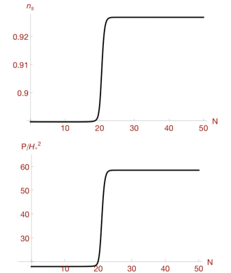
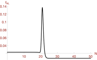
where the mass ratio $m_{\phi}/m_{\chi}=9$ and $m_{\chi}=10^{-5}M_{\mathrm{P}}$. We begin the calculation 50 e-folds before the end of inflation, with $\phi=8.2M_{\mathrm{P}}$ and $\chi=12.9M_{\mathrm{P}}$. In this model there is a single turn in field space. The turn is associated with a ‘spike’ in the amplitude of the local-mode bispectrum, typically measured by the parameter $f_{\mathrm{NL}}$; see Refs. Vernizzi and Wands (2006); Mulryne et al. (2010, 2011). The turn is also associated with a step in the amplitude of the power spectrum, $P$, and a similar step in the spectral index. In Figs. 1 and 2 these behaviours can be compared. We leave a careful analysis for future work.

Figure 3: Superhorizon evolution of the spectral index (top) and power spectrum of curvature perturbations (bottom) for a particular realization of a randomly generated potential.

Random potentials: nonmonotonic features. In this example we study an example of nonmonotonic evolution in the power spectrum. Nonmonotonic behaviour can occur for potentials which give rise to evolution less trivial than a single turn. We consider

$$V=\sum_{\begin{subarray}{c}1\leqslant m\leqslant 3\\ 1\leqslant n\leqslant 3\end{subarray}}\left[a_{mn}\cos{\left(m\phi+n\chi\right)}+b_{mn}\sin{\left(m\phi+n\chi\right)}\right].$$ (13)

The coefficients $a_{mn}$ and $b_{mn}$ are drawn randomly, making  a low-order Taylor approximation to a “generic” potential. Frazer & Liddle Frazer and Liddle (2011) used potentials of this kind to study the generic features of inflation in a randomly generated landscape.

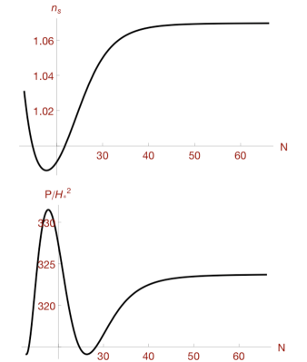
Fig. 3 shows the evolution of the power spectrum and spectral index in a specific realization of this model, both of which are nonmonotonic. Unlike the simple case of double quadratic inflation, the spectral index does not mirror the evolution of the power spectrum. This is a consequence of the different initial conditions for $n_{\alpha\beta}$ and $\Sigma_{\alpha\beta}$, which make $n_{\alpha\beta}$ grow more slowly than $\Sigma_{\alpha\beta}$. Eq. (8) implies that the net result is a decrease in $n_{s}-1$.

Figure 4: Superhorizon evolution of the spectral index (top) and power spectrum of curvature perturbations (bottom) for the exponential quadratic potential.

Exponential quadratic potential. Our final example exhibits a potential with unusual characteristics: the isocurvature modes do not decay and are present at the end of inflation. Therefore the curvature perturbation $\zeta$ will continue to evolve: it has not yet reached its “adiabatic limit” Elliston et al. (2011). The observable statistical properties of $\zeta$ in models of this type will depend on unknown details of the post-inflationary history, including the details of reheating. Therefore such models are less predictive than those which converge to their adiabatic limit during inflation. However, this is a question of calculability rather than principle. Models of this kind need not be intrinsically less interesting from the point of view of fundamental physics.

We use a model introduced by Byrnes et al. Byrnes et al. (2008), and studied in more detail by Elliston et al. Elliston et al. (2011). The potential is

$$V=V_{0}\chi^{2}\mathrm{e}^{{-\lambda\phi^{2}}}.$$ (14)

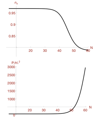
We choose $V_{0}=10^{-5}M_{\mathrm{P}}^{2}$ and $\lambda=0.05$, making our results comparable to Ref. Elliston et al. (2011) (the field values 55 e-folds before the end of inflation are $\phi=0.001M_{\mathrm{P}}$ and $\chi=16M_{\mathrm{P}}$). Fig. 4 shows that the power grows strongly from roughly 45 e-folds after horizon crossing, reflecting the divergence of nearby trajectories in field space described by Elliston et al. The corresponding evolution of $n_{s}$ is a stretched step. The amplitude of $P$ grows in comparison with $N_{,\alpha}N_{,\beta}n_{\alpha\beta}$, and the spectral index decreases significantly. Its value at the end of inflation is observationally unacceptable, but nothing can be concluded until the post-inflationary history is specified.

V Summary

Inflationary models motivated by high-energy physics frequently involve many light scalar fields with complicated potentials. For this reason, it is important to find efficient numerical tools with which to predict observable parameters.

In this paper, we have presented a simple method to compute the evolution of the spectral index in models where multi-field dynamics must be taken into account. Our approach uses a system of “transport equations”—a set of ordinary differential equations—to evolve the spectral indices $n_{\alpha\beta}$ of the 2-point functions of the canonically normalized scalar fields. These can be assembled into $n_{s}$ at the time of interest.

The transport equation for the indices $n_{\alpha\beta}$ is exactly the same as the equation used to transport the power spectra of the field perturbations. However, owing to its different initial conditions, its evolution is not trivially related to the evolution of the power spectra. Its behaviour depends on the characteristics of the potential. In §IV we exhibited specific examples that illustrate this behaviour. Although our examples were drawn from the class of 2-field models for reasons of simplicity, the method is valid for any number of fields.

In a model with $N$ fields, we require $N$ integrations to track the evolution of the centroid $\Phi_{\alpha}$, and $N(N+1)/2$ to evolve the two-point function $\Sigma_{\alpha\beta}$. To obtain a simple estimate, we assume the computational time is dominated by integration, and that integrating each component of $\Phi_{\alpha}$, $\Sigma_{\alpha\beta}$. Under these assumptions we can expect the time required to scale like $N(N+3)/2$.

Our method requires the introduction of another $N(N+1)/2$ equations to track the evolution of $n_{\alpha\beta}$. Assuming integration of $n_{\alpha\beta}$ takes comparable time to $\Sigma_{\alpha\beta}$ and $\Phi_{\alpha}$ (which should be a good approximation because $\Sigma_{\alpha\beta}$ and $n_{\alpha\beta}$ obey the same equation), the total time will now scale like $N(N+2)$. On the other hand, if we evolve the 2-point function at multiple scales in order to extract a numerical derivative by fitting a spline with $m$ points, then we will require $N+mN(N+1)/2$ integrations. Typically $m$ will be of order a few.

These simple estimates show that, asymptotically, either method has complexity $\operatorname{O}(N^{2})$. To obtain reasonable accuracy when extracting a numerical derivative, one might wish to fit a spline with several points. In this case one might expect the transport approach to be more efficient by a modest numerical factor. Although not dramatic, a small speed increase would certainly be worthwhile when accumulated over a large number of samples.

A similar approach could be adopted to calculate the scale dependence of any $n$-point function. The case of observational interest is likely to be the bispectrum, where one might wish to compute the running of the local-mode amplitude $f_{\mathrm{NL}}$ Byrnes et al. (2010); *Byrnes:2010xd. We leave this for future work.