DESY 11–227,  D0–TH 11/27,  SFB/CPP-11-70,  LPN11-67.
Two-loop operator matrix elements for massive fermionic local twist-2 operators in QED

Abstract:

We describe the calculation of the two–loop massive operator matrix elements with massive external fermions in QED. We investigate the factorization of the $O(\alpha^{2})$ initial state corrections to $e^{+}e^{-}$ annihilation into a virtual boson for large cms energies $s\gg m_{e}^{2}$ into massive operator matrix elements and the massless Wilson coefficients of the Drell-Yan process adapting the color coefficients to the case of QED, as proposed by Berends et. al. in Ref. [1]. Our calculations show explicitly that the representation proposed in Ref. [1] works at one-loop order and up to terms linear in $\ln(s/m^{2}_{e})$ at two-loop order. However, the two-loop constant part contains a few structural terms, which have not been obtained in previous direct calculations.

Ever since the operator product expansion formalism was applied to the analysis of deep inelastic scattering (DIS), there has been a lot of interest in the calculation of massive operator matrix elements at higher order in perturbation theory. Heavy flavor corrections to DIS structure functions are very important at small values of the Bjorken variable $x$ (where they contribute on the level of 20–40$\%$), and can be calculated in the limit $Q^{2}\gg m^{2}$ as a convolution of the corresponding massive operator matrix elements and the light flavor Wilson coefficients [2]. Here $Q^{2}$ denotes the virtuality of the gauge boson exchanged in DIS and $m$ is the mass of the heavy quark.

The scaling violations of the heavy flavor part in the structure functions $F_{2,L}(x,Q^{2})$ are very different from those of the light flavor contributions, and their knowledge is very important for precision measurements of $\Lambda_{\rm QCD}$ and the extraction of light parton densities. A semi-analytic calculation of the heavy flavor contributions was done in Ref. [3] at next-to-leading order for the full kinematic range, and a fast numerical implementation in Mellin space was given in [4]. Full analytic results in the asymptotic region $Q^{2}\gg m^{2}$ for the structure function $F_{2}^{Q\bar{Q}}(x,Q^{2})$ at $O(\alpha_{s}^{2})$ were derived in Ref. [2], and recently recalculated in [5]. In the same kinematic region, $F_{L}^{Q\bar{Q}}(x,Q^{2})$ was obtained at $O(\alpha_{s}^{3})$ in Ref. [6].

The $O(\alpha_{s}^{3})$ massive operator matrix elements are required in both cases and all but $O((m^{2}/Q^{2})^{k})$, $k>1$ contributions are found. In this approximation, the structure function $F_{2}(x,Q^{2})$ turns out to be very well described for $Q^{2}>20\rm GeV^{2}$, while for $F_{L}(x,Q^{2})$ this approximation only holds at large scales $Q^{2}>1000\,\rm GeV^{2}$.

More recently, there has been considerable progress in the calculation of the $O(\alpha_{s}^{3})$ heavy flavor contributions to the Wilson coefficients of the structure function $F_{2}(x,Q^{2})$ and the massive gluonic operator matrix elements. First, in Ref. [7] the $O(\alpha_{s}^{2}\varepsilon)$ corrections to these matrix elements were given. These corrections are required to perform the corresponding renormalization procedure at $O(\alpha_{s}^{3})$. Later, the calculation of these contributions for a number of fixed moments $N=2...10(12,14)$ at $O(\alpha_{s}^{3})$ has also been achieved in [8], and $O(\alpha_{s}^{3}n_{f})$ contributions were given in Ref. [9]. $O(\alpha_{s}^{2})$ and $O(\alpha_{s}^{3})$ heavy flavor contributions to transversity have also been obtained in [10].

On the other hand, massive operator matrix elements, and in particular those with a massive external fermion line, can also be applied to a different kind of problem, namely, the calculation of initial state QED corrections of scattering processes, such as $e^{+}e^{-}$ annihilation into a virtual gauge boson, using the renormalization group technique. A wealth of information about the Standard Model has been obtained in the past from electron–positron colliding beam experiments at different facilities around the world. In the future, projects like ILC [11] and CLIC [12] are planned to put the Standard Model to even more decisive tests and to reveal new physics [13]. In this context high-luminosity machines which operate at a narrow energy regime as DAFNE [14] and GIGA-Z [11, 13] at the $Z$-peak will offer much higher precision on rare processes.

The QED initial state radiation causes large corrections for various differential and integral scattering cross sections, depending on the sensitivity of the sub–system cross section with respect to kinematic rescaling of variables and has to be known at sufficient precision. Both for $e^{+}e^{-}$ annihilation at resonance peaks and the wings of resonances at very high luminosities, the knowledge of the $O(\alpha^{2})$ corrections is mandatory to cope with the experimental precision. While the $O(\alpha)$ corrections are known for a large amount of reactions, the corrections beyond the universal contributions $O((\alpha L)^{k}),1\leq k\leq 5$, see [15, 16], to higher orders, were only calculated once at two-loop order in Ref. [1]. Besides the logarithmic orders $O(\alpha^{2}L^{2},\alpha^{2}L)$ with $L=\ln(s/m_{e}^{2})$ and $m_{e}$ the electron mass, the constant terms $O(\alpha^{2})$ are of interest.

The renormalization group technique allows to decompose the scattering cross section $\sigma(e^{+}e^{-}$ $\rightarrow~{}V),~{}V=\gamma^{*},Z^{*}$ into massive operator matrix elements and massless Wilson coefficients. The fermion mass effects are contained in the former, while the sub-system hard scattering cross sections are calculated for massless particles. The corresponding massless Wilson coefficients are known from the literature [17, 18] for the Drell-Yan process. In [1] this method was used to derive all terms up to ${\rm O}(\alpha^{2}L)$ in addition to the direct calculation.

The differential scattering cross section can be written in the limit $s\gg m_{e}^{2}$ as a sum of three contributions [1]:

$$\frac{d{\sigma}_{e^{+}e^{-}}}{ds^{\prime}}=\frac{d{\sigma}_{e^{+}e^{-}}^{\rm I}}{ds^{\prime}}+\frac{d{\sigma}_{e^{+}e^{-}}^{\rm II}}{ds^{\prime}}+\frac{d{\sigma}_{e^{+}e^{-}}^{\rm III}}{ds^{\prime}}~{},$$ (1)

where the labels I, II and III refer to the flavor non-singlet terms with a single fermion line, those with an additional closed fermion line, and the pure-singlet terms, respectively. Here, $s^{\prime}$ denotes the invariant mass of the virtual vector boson and $s$ the cms energy of the process.

$$s^{\prime}=xs,\quad 0\leq x\leq 1.$$ (2)

It is convenient to write the scattering cross section in Mellin space by applying the integral transform

$$\widehat{\frac{d\sigma}{ds^{\prime}}}(N)=\int_{0}^{1}~{}dx~{}x^{N-1}~{}\frac{d\sigma}{ds^{\prime}}(xs)~{}.$$ (3)

Using the renormalization group method it can be shown that the three contributions in Eq. (1) can be expressed as [1, 19]

$$\widehat{\frac{d\sigma_{e^{+}e^{-}}^{\rm I}}{ds^{\prime}}} = \frac{1}{s}\widehat{\sigma^{(0)}}\Biggl{\{}1+a_{0}\left[P_{ee}^{(0)}{\bf L}+\tilde{\sigma}^{(0)}_{ee}+2\Gamma_{ee}^{(0)}\right]+a_{0}^{2}\Biggl{[}\frac{1}{2}{P_{ee}^{(0)}}^{2}{\bf L}^{2}$$ (4)

$$\phantom{\frac{1}{s}}+\left(P_{ee}^{(1),{\rm I}}+P_{ee}^{(0)}\left(\tilde{\sigma}_{ee}^{(0)}+2\Gamma_{ee}^{(0)}\right)\right){\bf L}+2\Gamma_{ee}^{(1),{\rm I}}+\tilde{\sigma}_{ee}^{(1),{\rm I}}+2\Gamma_{ee}^{(0)}\tilde{\sigma}_{ee}^{(0)}+{\Gamma_{ee}^{(0)}}^{2}\Biggr{]}\Biggr{\}}~{},$$

$$\widehat{\frac{d\sigma_{e^{+}e^{-}}^{\rm II}}{ds^{\prime}}} = \frac{1}{s}\widehat{\sigma^{(0)}}a_{0}^{2}\Biggl{\{}-\frac{\beta_{0}}{2}P_{ee}^{(0)}{\bf L}^{2}+\Biggl{[}P_{ee}^{(1),{\rm II}}-\beta_{0}\tilde{\sigma}_{ee}^{(0)}\Biggr{]}{\bf L}+2\Gamma_{ee}^{(1),{\rm II}}+\tilde{\sigma}_{ee}^{(1),{\rm II}}\Biggr{\}}~{},$$ (5)

$$\widehat{\frac{d\sigma_{e^{+}e^{-}}^{\rm III}}{ds^{\prime}}} = \frac{1}{s}\widehat{\sigma^{(0)}}a_{0}^{2}\Biggl{\{}\frac{1}{4}P_{e\gamma}^{(0)}P_{\gamma e}^{(0)}{\bf L}^{2}+\Biggl{[}P_{ee}^{(1),{\rm III}}+P_{\gamma e}^{(0)}\tilde{\sigma}_{e\gamma}^{(0)}+\Gamma_{\gamma e}^{(0)}P_{e\gamma}^{(0)}\Biggr{]}{\bf L}$$ (6)

$$\phantom{\frac{1}{s}\widehat{\sigma^{(0)}}a_{0}^{2}}+2\Gamma_{ee}^{(1),{\rm III}}+\tilde{\sigma}_{ee}^{(1),{\rm III}}+2\tilde{\sigma}_{e\gamma}^{(0)}\Gamma_{\gamma e}^{(0)}\Biggr{\}}~{},$$

where ${\bf L}=\ln(s/m_{e}^{2})+\ln(x)$, and $\widehat{\sigma^{(0)}}$ is the Born cross section. The quantities $P_{ij}^{(0)}$ and $\tilde{\sigma}_{ij}^{(0)}$ are the LO splitting functions and LO Wilson coefficients, respectively, while at NLO they are denoted by $P_{ee}^{(1)}$ and $\tilde{\sigma}_{ee}^{(1)}$. $\Gamma_{ij}^{(0)}$ and $\Gamma_{ee}^{(1)}$ are the one-loop and two-loop constant terms of the massive operator matrix elements, respectively. The labels I, II and III appear in $P_{ee}^{(1)}$, $\tilde{\sigma}_{ee}^{(1)}$ and $\Gamma_{ee}^{(1)}$ corresponding to the three possible contributions. The constant $\beta_{0}$ is the first coefficient in the expansion of the QED $\beta$-function.

The splitting functions up to $O(\alpha^{2})$ are well known [20], and as we mentioned before, so are the massless Wilson coefficients [17, 18]. Here we present the missing ingredient needed to complete the decomposition of the scattering cross section according to Eqs. (4–6), namely, the $O(\alpha^{2})$ massive operator matrix elements. Details on the calculation can be found in Ref. [19].

The bare operator matrix elements are given by

$$\hat{\hat{A}}_{ij}\left(\frac{{m}^{2}_{e}}{\mu^{2}},\varepsilon,N\right)=\delta_{ij}+\sum_{k=1}^{\infty}\hat{a}^{k}\hat{\hat{A}}_{ij}^{(k)}\left(\frac{{m}^{2}_{e}}{\mu^{2}},\varepsilon,N\right)~{},$$ (7)

where $\hat{a}$ is the unrenormalized coupling constant. The double hat means that the quantity is completely unrenormalized. The complete renormalization procedure includes charge renormalization, wave function renormalization and the renormalization of the composite operators. We need the inclusion of some counterterm diagrams in the case of process I. The electron mass is renormalized on-shell, $p^{2}=m^{2}_{e}$, with $p$ the momentum of the external fermion, which means that no collinear singularities will appear.

The wave function renormalization was performed using the Z-factors coming from the fermion self-energy, see Fig. 1. Since we have a massive fermion in the external legs, the coupling constant was first obtained in the MOM-scheme, after which we transform to the $\overline{\rm MS}$ scheme using

$$a^{\rm MOM}=a^{\overline{\rm MS}}+\frac{4}{3}\ln\left(\frac{m_{e}^{2}}{\mu^{2}}\right){a^{\overline{\rm MS}}}^{2}+O\left({a^{\overline{\rm MS}}}^{3}\right)~{}.$$ (8)

Figure 1: The self-energy diagrams.

We perform the calculation in $D=4+\varepsilon$ dimensions. It can be shown that after wave function and charge renormalization, keeping the charge in the MOM-scheme, the two-loop OMEs, denoted by a single hat, are given by

$$\hat{A}_{ee}^{\rm I} = a^{\sf MOM}S_{\varepsilon}\left(\frac{m^{2}_{e}}{\mu^{2}}\right)^{\varepsilon/2}\left[-\frac{1}{\varepsilon}P_{ee}^{(0)}+\Gamma_{ee}^{(0)}+\varepsilon\overline{\Gamma}^{(0)}_{ee}\right]$$ (9)

$$+{a^{\sf MOM}}^{2}S_{\varepsilon}^{2}\left(\frac{m^{2}_{e}}{\mu^{2}}\right)^{\varepsilon}\left\{\frac{1}{2\varepsilon^{2}}P_{ee}^{(0)}\otimes P_{ee}^{(0)}-\frac{1}{2\varepsilon}\left[P_{ee}^{(1),\rm I}+2\Gamma_{ee}^{(0)}\otimes P_{ee}^{(0)}\right]+\hat{\Gamma}_{ee}^{(1),\rm I}\right\}~{},$$

$$\hat{A}_{ee}^{\rm II} = {a^{\sf MOM}}^{2}S_{\varepsilon}^{2}\left(\frac{m^{2}_{e}}{\mu^{2}}\right)^{\varepsilon}\left\{\frac{1}{2\varepsilon^{2}}2\beta_{0}P_{ee}^{(0)}-\frac{1}{2\varepsilon}\left[P_{ee}^{(1),\rm II}+4\beta_{0}\Gamma_{ee}^{(0)}\right]+\hat{\Gamma}_{ee}^{(1),\rm II}\right\}~{},$$ (10)

$$\hat{A}_{ee}^{\rm III} = {a^{\sf MOM}}^{2}S_{\varepsilon}^{2}\left(\frac{m^{2}_{e}}{\mu^{2}}\right)^{\varepsilon}\left\{\frac{1}{2\varepsilon^{2}}P_{e\gamma}^{(0)}\otimes P_{\gamma e}^{(0)}-\frac{1}{2\varepsilon}\left[P_{ee}^{(1),\rm III}+2\Gamma_{\gamma e}^{(0)}\otimes P_{e\gamma}^{(0)}\right]+\hat{\Gamma}_{ee}^{(1),\rm III}\right\}~{}.$$ (11)

For the final renormalization step, i.e., the renormalization of the composite operators we just need to include the corresponding inverse Z-factors, $Z^{(1)}_{ij}$, after which the completely renormalized OMEs are given by

$$A_{ij}^{\sf MOM}=\delta_{ij}+a^{\sf MOM}\left[\hat{A}_{ij}^{(1)}+Z_{i,j}^{-1,(1)}\right]+{a^{\sf MOM}}^{2}\left[\hat{A}_{ij}^{(2)}+Z_{i,j}^{-1,(2)}+Z_{i,j}^{-1,(1)}\hat{A}_{ij}^{(1)}\right]+O({a^{\sf MOM}}^{3})~{}.$$ (12)

The Feynman diagrams required for process I are shown in Fig. 2. As it was mentioned before, in order to renormalize the corresponding OMEs for this process, we need to include also the counterterm diagrams shown in Fig. 3, where the black stars represent the counterterm vertices in QED. The diagrams are calculated using the standard Feynman rules for the operator insertions, and projecting the resulting numerators in the integrands with the factor $(\not\!\!p+m)/4$, after which we take the trace. The program FORM [21] was used to decompose the diagrams as a linear combination of integrals with different powers of propagators, which arise after canceling as many terms as possible in the numerator against the propagators. The most complicated integrals appearing in the expressions are those where all five propagators are present. These can be computed using integration by parts identities to express them in terms of 4-propagator integrals. The resulting integrals were checked by several means, including their representation in terms of Mellin-Barnes integrals, cf. [19].

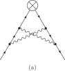
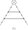
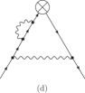
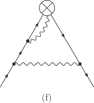
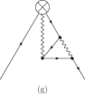
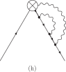
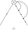
Figure 2: Feynman diagrams for the calculation of the massive two-loop operator matrix elements $A^{(2),{\rm I}}_{ee}$.

Figure 3: Counterterm diagrams. The black stars represent the counterterm vertices.

The constant contributions to process I in Eq. (9) is given in $x$-space by [19]

$$\hat{\Gamma}^{(1),\rm I}_{ee} = \frac{1+3x^{2}}{1-x}\left[6\zeta_{2}\ln(x)-8\ln(x){\rm Li}_{2}(1-x)-4\ln^{2}(x)\ln(1-x)\right]+\left({122\over 3}x+22+{32\over 1-x}\right)\zeta_{2}$$ (13)

$$+16\frac{1+x^{2}}{1-x}\left[2{\rm Li}_{3}(-x)-\ln(x){\rm Li}_{2}(-x)\right]+{80\over 3(1-x)}+56(1+x)\zeta_{2}\ln(1-x)+\left({22\over 3}x+32\right.$$

$$\left.+{64\over 3(1-x)^{2}}-{51\over 1-x}-{16\over 3(1-x)^{3}}\right)\ln^{2}(x)-(92+20x)\ln^{2}(1-x)+\left({178\over 3}+{64\over 3(1-x)^{2}}\right.$$

$$\left.-36x-{140\over 3(1-x)}-{48\over 1+x}\right)\ln(x)-\frac{1}{3}(1+x)\ln^{3}(x)+4\frac{x^{2}-8x-6}{1-x}\ln(x)\ln(1-x)$$

$$-2\frac{1+17x^{2}}{1-x}\ln(x)\ln^{2}(1-x)-\frac{112}{3}(1+x)\ln^{3}(1-x)+32\frac{1+x}{1-x}\left[\ln(x)\ln(1+x)+{\rm Li}_{2}(-x)\right]$$

$$-22x-{62\over 3}-4\frac{13x^{2}+9}{1-x}{\rm S}_{1,2}(1-x)+4\frac{5-11x^{2}}{1-x}\left[\ln(1-x){\rm Li}_{2}(1-x)-{\rm Li}_{3}(1-x)-2\zeta_{3}\right]$$

$$+\frac{4(16x^{2}-10x-27)}{3(1-x)}{\rm Li}_{2}(1-x)+14(x-2)\ln(1-x)+\left(16-52\zeta_{2}+128\zeta_{3}\right){\cal D}_{0}(x)$$

$$+\left(8-112\zeta_{2}\right){\cal D}_{1}(x)+120{\cal D}_{2}(x)+{224\over 3}{\cal D}_{3}(x)+\left[{433\over 8}+58\zeta_{3}+\left({37\over 2}-48\ln(2)\right)\zeta_{2}\right.$$

$$\left.-{67\over 45}\pi^{4}\right]\delta(1-x)+(-1)^{n}\left\{\frac{4(x^{2}+10x-3)}{3(1+x)}\left(\zeta_{2}+2{\rm Li}_{2}(-x)+2\ln(x)\ln(1+x)\right)\right.$$

$$+\frac{2(1-x)(45x^{2}+74x+45)}{3(1+x)^{2}}+\frac{2(9+12x+30x^{2}-20x^{3}-15x^{4})}{3(1+x)^{3}}\ln(x)$$

$$+\frac{1+x^{2}}{1+x}\left[\phantom{\rule{0.28453pt}{15.93347pt}}\!\right.8\zeta_{2}\ln(x)-24\zeta_{2}\ln(1+x)+36\zeta_{3}-\frac{2}{3}\ln^{3}(x)+40{\rm Li}_{3}(-x)-4\ln^{2}(x)\ln(1+x)$$

$$-24\ln(x)\ln^{2}(1+x)-24\ln(x){\rm Li}_{2}(-x)-48\ln(1+x){\rm Li}_{2}(-x)-8\ln(x){\rm Li}_{2}(1-x)$$

$$-16{\rm S}_{1,2}(1-x)-48{\rm S}_{1,2}(-x)\left.\!\phantom{\rule{0.28453pt}{15.93347pt}}\right]-\frac{16(x^{4}+12x^{3}+12x^{2}+8x+3)}{3(1+x)^{3}}{\rm Li}_{2}(1-x)$$

$$\left.+4x\frac{1-x-5x^{2}+x^{3}}{(1+x)^{3}}\ln^{2}(x)\right\}~{},$$

where ${\rm Li}_{n}(x)$ and ${\rm S}_{n,p}(x)$ are the well known polylogarithm and Nielsen functions, and

$${\cal D}_{k}(x)=\left(\frac{\ln^{k}(1-x)}{1-x}\right)_{+}.$$

For process II we need the diagrams in Fig. 4. These are relatively easy to compute, since they involve a one-loop insertion. The result for the constant term of process II in Eq. (10) is given by [19]

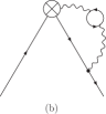
Figure 4: Feynman diagrams for the calculation of the massive two-loop operator matrix elements $A^{(2),{\rm II}}_{ee}$.

$$\hat{\Gamma}^{(1),\rm II}_{ee} = {76\over 27}x-{572\over 27}-\left(12x+{4\over 3}+{8\over 1-x}+{32\over 9(1-x)^{2}}-{160\over 9(1-x)^{3}}+{64\over 9(1-x)^{4}}\right)\ln(x)+{128\over 9(1-x)^{2}}$$ (14)

$$+{80\over 27(1-x)}-{64\over 9(1-x)^{3}}-{2(1+x^{2})\over 3(1-x)}\ln^{2}(x)+{16\over 3}(1+x)\left(\ln(1-x)+\ln^{2}(1-x)+{1\over 4}\zeta_{2}\right)$$

$$+\left({224\over 27}-{8\over 3}\zeta_{2}\right){\cal D}_{0}(x)-{32\over 3}\left({\cal D}_{1}(x)+{\cal D}_{2}(x)\right)+\left({8\over 3}\zeta_{3}-10\zeta_{2}+{1411\over 162}\right)\delta(1-x).$$

In the case of process III, we need the pure singlet diagrams shown in Fig. 5. These can be calculated using the corresponding one-loop operator insertions, which were given in Ref. [22]. The result for the constant term appearing in Eq. (11) is [19]

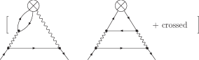
Figure 5: Feynman diagrams for the calculation of the massive two-loop operator matrix elements $A^{(2),{\rm III}}_{ee}$.

$$\hat{\Gamma}^{(1),\rm III}_{ee} = {2\over x}(1-x)(4x^{2}+13x+4)\zeta_{2}+{1\over 3x}(8x^{3}+135x^{2}+75x+32)\ln^{2}(x)+\left[{304\over 9x}-{80\over 9}x^{2}-{32\over 3}x\right.$$ (15)

$$\left.+108-{32\over 1+x}-{64(1+2x)\over 3(1+x)^{3}}\right]\ln(x)+50-{224\over 27}x^{2}-{182\over 3}x-{32\over 1+x}+{64\over 3(1+x)^{2}}+{800\over 27x}$$

$$+16{1-x\over 3x}(x^{2}+4x+1)\left[2\ln(x)\ln(1+x)-{\rm Li}_{2}(1-x)+2{\rm Li}_{2}(-x)\right]+(1+x)\left[\phantom{\rule{0.28453pt}{15.93347pt}}\!\right.4\zeta_{2}\ln(x)$$

$$+{14\over 3}\ln^{3}(x)-32\ln(x){\rm Li}_{2}(-x)-16\ln(x){\rm Li}_{2}(x)+64{\rm Li}_{3}(-x)+32{\rm Li}_{3}(x)+16\zeta_{3}\left.\!\phantom{\rule{0.28453pt}{15.93347pt}}\right]~{}.$$

Our calculations show explicitly that the operator matrix elements satisfy the relations given in Eqs. (9–11) for the pole terms, which automatically guarantees that the decomposition given in Eqs. (4–6) holds for the logarithmic terms, as found in Ref. [1]. Furthermore, we have verified that the first moment of the operator matrix elements vanishes, including the constant terms given in Eqs. (13-15), so they obey fermion number conservation as they should. This provides a highly non-trivial check of our results. However, when we assemble the final result for the constant terms in Eqs. (4–6) by including the massless Wilson coefficients, we observe that, although many of terms appearing in Ref. [1] appear in our results, a few structural terms, such as terms proportional to $1/(1-x)^{3}$ and $\ln(x)/(1-x)^{4}$, also appear, which were not present in the result given in [1]. This result appears in contrast to the case of massless external fermions and boson lines, where the corresponding cross sections have been shown to factorize, including the constant terms, as can be seen in Refs. [2, 3, 5, 6, 23]. The issue requires further investigation in order to elucidate the reasons for this.

References

• [1] F. A. Berends, W. L. van Neerven and G. J. H. Burgers, Nucl. Phys. B 297 (1988) 429 [Erratum-ibid. B 304 (1988) 921]; For process II: B. A. Kniehl, M. Krawczyk, J. H. Kühn and R. G. Stuart, Phys. Lett. B 209 (1988) 337.
• [2] M. Buza, Y. Matiounine, J. Smith, R. Migneron and W. L. van Neerven, Nucl. Phys. B 472 (1996) 611 [hep-ph/9601302].
• [3] E. Laenen, S. Riemersma, J. Smith and W. L. van Neerven, Nucl. Phys. B 392 (1993) 229.
• [4] S. I. Alekhin and J. Blümlein, Phys. Lett. B 594 (2004) 299 [hep-ph/0404034].
• [5] I. Bierenbaum, J. Blümlein and S. Klein, Nucl. Phys. B 780 (2007) 40 [hep-ph/0703285].
• [6] J. Blümlein, A. De Freitas, W. L. van Neerven and S. Klein, Nucl. Phys. B 755 (2006) 272 [hep-ph/0608024].
• [7] I. Bierenbaum, J. Blümlein, S. Klein and C. Schneider, Nucl. Phys. B 803 (2008) 1 [arXiv:0803.0273 [hep-ph]];
I. Bierenbaum, J. Blümlein and S. Klein, Phys. Lett. B 672 (2009) 401 [arXiv:0901.0669 [hep-ph]].
• [8] I. Bierenbaum, J. Blümlein and S. Klein, Nucl. Phys. B 820 (2009) 417 [arXiv:0904.3563 [hep-ph]].
• [9] J. Ablinger, J. Blümlein, S. Klein, C. Schneider and F. Wißbrock, Nucl. Phys. B 844 (2011) 26 [arXiv:1008.3347 [hep-ph]].
• [10] J. Blümlein, S. Klein and B. Tödtli, Phys. Rev. D 80 (2009) 094010 [arXiv:0909.1547 [hep-ph]].
• [11] J. A. Aguilar-Saavedra et al. [ECFA/DESY LC Physics Working Group], hep-ph/0106315.
• [12] S. van der Meer, The CLIC Project and the Design for an $e^{+}e^{-}$ Collider, CLIC-NOTE-68, (1988).
• [13] E. Accomando et al. [ECFA/DESY LC Physics Working Group], Phys. Rept.  299 (1998) 1 [hep-ph/9705442].
• [14] P. Franzini and M. Moulson, Ann. Rev. Nucl. Part. Sci.  56 (2006) 207 [hep-ex/0606033].
• [15] M. Skrzypek, Acta Phys. Polon. B 23 (1992) 135; M. Jezabek, Z. Phys. C 56 (1992) 285; M. Przybycien, Acta Phys. Polon. B 24 (1993) 1105 [hep-th/9511029]; A. B. Arbuzov, Phys. Lett. B 470 (1999) 252 [hep-ph/9908361].
• [16] J. Blümlein and H. Kawamura, Eur. Phys. J. C 51 (2007) 317 [hep-ph/0701019]; J. Blümlein and H. Kawamura, Nucl. Phys. B 708 (2005) 467 [hep-ph/0409289].
• [17] R. Hamberg, W. L. van Neerven and T. Matsuura, Nucl. Phys. B 359 (1991) 343 [Erratum-ibid. B 644 (2002) 403].
• [18] R. V. Harlander and W. B. Kilgore, Phys. Rev. Lett.  88 (2002) 201801 [hep-ph/0201206];
Further typographical errors are corrected in van Neerven’s code corresponding to [17]. A representation in Mellin space was given in: J. Blümlein and V. Ravindran, Nucl. Phys. B 716 (2005) 128 [arXiv:hep-ph/0501178 [hep-ph]].
• [19] J. Blümlein, A. De Freitas and W. van Neerven, Nucl. Phys. B 855 (2012) 508 [arXiv:1107.4638 [hep-ph]].
• [20] E. G. Floratos, D. A. Ross and C. T. Sachrajda, Nucl. Phys. B 129 (1977) 66 [Erratum-ibid. B 139 (1978) 545]; Nucl. Phys. B 152 (1979) 493; A. Gonzalez-Arroyo, C. Lopez and F. J. Yndurain, Nucl. Phys. B 153 (1979) 161; A. Gonzalez-Arroyo and C. Lopez, Nucl. Phys. B 166 (1980) 429; E. G. Floratos, C. Kounnas and R. Lacaze, Nucl. Phys. B 192 (1981) 417; G. Curci, W. Furmanski and R. Petronzio, Nucl. Phys. B 175 (1980) 27; W. Furmanski and R. Petronzio, Phys. Lett. B 97 (1980) 437; R. Hamberg and W. L. van Neerven, Nucl. Phys. B 379 (1992) 143; R. K. Ellis and W. Vogelsang, hep-ph/9602356; S. Moch and J. A. M. Vermaseren, Nucl. Phys. B 573 (2000) 853 [hep-ph/9912355].
• [21] J. A. M. Vermaseren, math-ph/0010025.
• [22] S. W. G. Klein, Mellin moments of heavy flavor contributions to $F_{2}(x,Q^{2})$ at NNLO, PhD Thesis, TU Dortmund, September 2009, arXiv:0910.3101 [hep-ph].
• [23] M. Buza, Y. Matiounine, J. Smith and W. L. van Neerven, Eur. Phys. J. C 1 (1998) 301 [arXiv:hep-ph/9612398 [hep-ph]]; Nucl. Phys. B 485 (1997) 420 [hep-ph/9608342]; I. Bierenbaum, J. Blümlein and S. Klein, PoSDIS 2010 (2010) 148 [arXiv:1008.0792 [hep-ph]].