Limitations of Perturbative Techniques in the Analysis of Rhythms and Oscillations

Abstract

Perturbation theory is an important tool in the analysis of oscillators and their response to external stimuli. It is predicated on the assumption that the perturbations in question are “sufficiently weak”, an assumption that is not always valid when perturbative methods are applied. In this paper, we identify a number of concrete dynamical scenarios in which a standard perturbative technique, based on the infinitesimal phase response curve (PRC), is shown to give different predictions than the full model. Shear-induced chaos, i.e., chaotic behavior that results from the amplification of small perturbations by underlying shear, is missed entirely by the PRC. We show also that the presence of “sticky” phase-space structures tend to cause perturbative techniques to overestimate the frequencies and regularity of the oscillations. The phenomena we describe can all be observed in a simple 2D neuron model, which we choose for illustration as the PRC is widely used in mathematical neuroscience.

Introduction

Rhythmic activity is commonplace in biological phenomena: the spontaneous beating of heart cells in culture [10], the synchronization of flashing fireflies [27], and central pattern generators in animal locomotion [3], and calcium oscillations that underlie a plethora of cellular responses (ranging from muscle contraction to neurosecretion) [32] are just a few examples (see, e.g., [11] and [38] for many more). Mathematical models of biological oscillations often provide useful insights into the underlying biological process; for example, they can explain the observed robustness of circadian rhythms [38] and of population cycles [25], and can be used to infer plausible structures for central pattern generator networks based on locomotion gaits [12]. Analyzing models of biological oscillations, however, is generally not easy: the mechanisms underlying biological rhythms are varied and complex, and this complexity is reflected in the corresponding mathematical models. Indeed, models of biological oscillators are often high dimensional, highly nonlinear, and have uncertain parameters, all of which make them challenging to study.

Perturbation theory, long a staple of applied mathematics, provides a practical solution in many situations. Mathematically, robust oscillations correspond to attracting limit cycles in phase space. If the stimuli involved are not too strong, then one is justified in viewing trajectories of the forced system as perturbations of the original limit cycle. When judiciously applied, such perturbative analyses can yield a great deal of insight and useful quantitative predictions. For oscillators, a good example of an effective perturbation technique is that of infinitesimal phase response curves (PRCs) and associated phase reductions [7]. The infinitesimal PRC of an oscillator records the phase change that results from an applied perturbation. Given an oscillator, there are many ways to obtain its infinitesimal PRC: in addition to analytical perturbation techniques, there are efficient numerical methods for constructing PRCs; the entire PRC itself can even be inferred directly from experimental data. Moreover, PRC-based techniques require only tracking just the phase of the oscillator, thereby greatly reducing complexity. They are used in many areas of mathematical biology, but especially in computational neuroscience, as they yield direct predictions about the modulation of spike timing and frequency by external stimuli. Furthermore, they allow one to make predictions for weakly-coupled networks [16, 31] .

However, as is well known, perturbation methods do not always correctly reflect the true dynamical picture, as they systematically overlook certain aspects of the dynamics. In using perturbation theory, one assumes that the perturbation is small, an assumption that is not always valid in applications. In this paper, we identify a number of concrete scenarios in which PRCs and phase reductions give predictions different from that of the full model. One situation is when the perturbation causes the trajectory to leave the basin of attraction of the limit cycle, which can occur even with moderately weak forcing. But even without leaving the basin, more subtle effects can lead perturbation theory astray, giving — to varying degrees — incorrect predictions. These situations include the presence of “sticky” invariant phase-space structures near a limit cycle, which can cause perturbation theory to overestimate the regularity and frequency of a stimulated oscillator. We will also show that dynamical shear in a neighborhood of the oscillator can cause it to behave chaotically when forced. These scenarios cannot be captured by infinitesimal phase reductions.

The scenarios described in this paper are relevant for general oscillators, but in view of the popularity of PRC-based techniques in neuroscience, we will illustrate our ideas using the Morris-Lecar (ML) neuron model [8, 9]. This widely-used model provides a convenient and flexible example because of its low dimensionality and rich bifurcation structure. The phenomena of interest are not hard to find in certain ML regimes; they do not require stringent tuning of parameters. We point out also that while we focus here on single neuron models, our findings remain relevant for oscillators operating within networks.

This paper is organized as follows: In Sect. 1, we review some relevant mathematical background, including brief discussions of phase response theory and “shear-induced chaos”, a general mechanism for producing chaotic behavior in driven oscillators. Sect. 2 introduces the ML model and some relevant ideas from computational neuroscience. In the last three sections, certain regimes of the ML model are used to demonstrate how perturbative techniques sometimes do not correctly predict the behavior of the full model. Sect. 3 contains an example in which the infinitesimal PRC gives no hint of the strange attractor in the full model. Sects. 4 and 5 illustrate how the presence of nearby invariant structures can impact neuronal response in ways that cannot be captured by PRCs alone.

1 Mathematical background

The general setting for this section is a nonlinear oscillator modeled by an $n$-dimensional ODE $\dot{x}=f(x)$ with a limit cycle $\gamma$ . We assume throughout that $\gamma$ is not only attractive as a periodic orbit but hyperbolic, i.e., its Floquet multipliers have absolute values $<1$. The period of $\gamma$ is denoted ${\rm Per}(\gamma)$.

1.1 Phase response curves and phase reductions

This section contains a brief review of a perturbation technique for oscillators known as (infinitesimal) phase response theory. For more details and many applications, see, e.g., [9, 11, 13, 38].

First, we fix a notion of “phase” on the oscillator: Fix a reference point $x_{*}\in\gamma$, and declare its phase to be $\psi(x_{*})=0$. For any other point $x\in\gamma$, the phase $\psi(x)$ can be defined to be the amount of time to go from $x_{*}$ to $x$ along the cycle $\gamma$ . Next we extend this notion to a neighborhood of $\gamma$. It is a mathematical fact that $\psi$ extends uniquely to a smooth function such that for all solutions $x$ with $x(0)$ near $\gamma$, $\frac{d}{dt}\psi(x(t))=1$ . Thus $\psi$ serves as a kind of “clock” for tracking the passage of time along trajectories near $\gamma$.

Our goal is to describe what happens to the phase when a time-dependent perturbation is applied. Let $\theta(t):=\psi(x(t))$, where $x$ is a perturbed trajectory. We would like an approximate equation for $\theta(t)$ . Rather than doing this for general perturbations, we consider a perturbed equation of the form

$$\dot{x}=f(x)+I(t)\hat{k}~{},$$ (1)

where $x(t)\in\mathbb{R}^{n}$ , $I$ is a scalar signal, and $\hat{k}\in\mathbb{R}^{n}$ is a constant vector. (In neuroscience applications, for example, one of the variables usually represents the membrane voltage, and this is typically the only variable that can be directly affected by external perturbations.) Now let $\xi:\mathbb{R}\to\mathbb{R}^{n}$ be a periodic solution to the “adjoint equation”

$$\dot{\xi}(t)=-Df(\gamma(t))^{T}\cdot\xi(t)~{},$$ (2)

where $\gamma(t)$ denotes an orbit parametrizing the cycle $\gamma$ , and let $\Delta(\theta):=\xi(\theta)\cdot\hat{k}$ . Under the normalization condition $\xi(0)\cdot f(0)=1$, it can be shown (see, e.g., [9]) that if $x$ is a solution of Eq. (1) and $I=O(\varepsilon)$ for a small parameter $\varepsilon$, then $\theta$ satisfies

$$\dot{\theta}=1+\Delta(\theta)I(t)+O(\varepsilon^{2})~{}.$$ (3)

Truncating all terms of $O(\varepsilon^{2})$ in Eq. (3) yields an equation for $\theta$, the phase reduction of Eq. (1). The function $\Delta$ is the infinitesimal phase response curve (PRC).

For systems that are near a bifurcation, the above procedure can be used to derive analytical approximations of the PRC via normal forms [2]. In more general situations (where there are few practical analytical techniques), one can obtain PRCs through numerical computation, or even directly from experimental measurements (see, e.g., [29, 28, 38] and references therein). This flexibility and accessibility is part of its appeal in mathematical biology, and in neuroscience in particular.

Stochastic forcing. The basic methodology of infinitesimal phase response curves can be extended to systems driven by stochastic forcing. That is, suppose that in addition to a deterministic forcing, we add a second white-noise term:

$$\dot{x}=f(x)+(I(t)+\beta\dot{W})~{}\hat{k}~{};\qquad\dot{W}=\mbox{white noise.}$$

In [24], Ly and Ermentrout show that with the above forcing, $\theta$ satisfies the equation

$$\dot{\theta}=1+\Delta(\theta)I(t)+\frac{\beta^{2}}{2}\Delta(\theta)\Delta^{\prime}(\theta)+\beta\Delta(\theta)\dot{W}~{}~{}+~{}~{}(\mbox{higher order terms})~{},$$ (4)

assuming both $\varepsilon$ and $\beta$ are small.

Eq. (4) can be used to derive a number of quantities of interest. For example, if we view Eq. (4) as modeling a neuron that “fires” whenever $\theta=0$ , then a result of Ly and Ermentrout states that the firing rate resulting from a constant forcing $I(t)\equiv\varepsilon$ is

$$r(\varepsilon)=1+\varepsilon\bar{\Delta}+\varepsilon^{2}\int_{0}^{{\rm Per}(\gamma)}\Big{(}{\bar{\Delta}}^{2}-\Delta^{2}(\theta)\Big{)}~{}d\theta+\frac{\beta^{4}}{4}\int_{0}^{{\rm Per}(\gamma)}\Delta^{2}(\theta)\big{(}\Delta^{\prime}(\theta)\big{)}^{2}~{}d\theta+O(\varepsilon^{3})~{},$$ (5)

to leading order in $\beta$ . In the above, $\bar{\Delta}=\int_{0}^{{\rm Per}(\gamma)}\Delta(\theta)~{}d\theta$.

Remark on terminology. Other variants of the PRC exist for finite-size perturbations. In this paper, the term “PRC” will always mean the infinitesimal phase response curve.

1.2 When do phase reductions work, and when might they fail?

Because the PRC is defined in terms of a vector field $f$ and its derivative along a limit cycle $\gamma$ (see Eq. (2)), it can only contain information about the flow in an infinitesimal neighborhood of $\gamma$. We discuss briefly in this subsection a few scenarios in which the behavior of the flow a finite distance away from $\gamma$ can have a dramatic effect on the oscillator’s response. These ideas are illustrated in concrete examples in Sects. 3 – 5.

(1) Leaving the basin of $\gamma$. The simplest possible way for something to go wrong is when the forcing carries a phase point outside of the basin of attraction of $\gamma$. If $\Phi_{t}$ denotes the unforced flow, then the basin of $\gamma$, denoted ${\rm Basin}(\gamma)$, is defined to be the set of all phase points $x$ such that $\Phi_{t}(x)\to\gamma$ as $t\to\infty$. Once a perturbation, say in the form of a “kick”, causes a trajectory to leave ${\rm Basin}(\gamma)$, what it does may depend on dynamical structures far away from $\gamma$. For example, if the system is bistable, or multi-stable, i.e., it has more than one attracting set, which can be in the form of a stationary point, a limit cycle, or something more complicated, then an “escaped” trajectory can end up near one of these structures, and in time, it may – or may not – get kicked back into ${\rm Basin}(\gamma)$. Needless to say, the behavior of such a trajectory bears little resemblance to that predicted by the PRC. This scenario must be taken into consideration when the forcing is strong relative to the distance of $\partial({\rm Basin}(\gamma))$ to $\gamma$. (Here $\partial({\rm Basin}(\gamma))$ is the boundary of ${\rm Basin}(\gamma)$.)

(2) Invariant structures and “trapping”. Even without venturing outside of ${\rm Basin}(\gamma)$, a perturbed trajectory that comes near $\partial({\rm Basin}(\gamma))$ can be nontrivially affected by certain dynamical structures in $\partial({\rm Basin}(\gamma))$. These structures may seem innocuous – they are non-attracting – but as we will see, they can seriously impact the surrounding dynamics. Consider, for example, a saddle fixed point of the unperturbed flow. An orbit that comes near it will, under the unperturbed flow, remain near it for some duration of time (depending on the ratios of the eigenvalues of the linearized flow at that point). Since an invariant structure is typically not truly invariant for the perturbed flow, a perturbed trajectory that gets near it will likely escape eventually and return to $\gamma$. However, the escape time can be quite long, and this effect cannot be captured by phase reductions. The tendency to remain near invariant structures can be mitigated by the forcing when the forcing acts to push trajectories away; by the same token, it can also be magnified if the forcing “conspires” to keep trajectories in a region. Indeed, there is no reason why a forcing cannot – by itself – create trapping regions within the basin of $\gamma$ if the attraction to $\gamma$ is weak compared to the forcing.

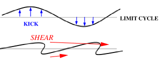
Figure 1: The stretch-and-fold action of a kick followed by relaxation in the presence of shear.

(3) Shear-induced chaos. This is yet another dynamical phenomenon that cannot be captured by (infinitesimal) PRCs. This phenomenon is illustrated in Fig. 1. In each of the two pictures, $\gamma$ is represented by the horizontal line. Shear refers to the differential in the horizontal component of the velocity as one moves vertically up in the phase space; here points above $\gamma$ move around $\gamma$ faster than points below. Suppose that an impulsive perturbation, or “kick,” applied in such a situation produces a “bump” in $\gamma$. As the flow relaxes, this “bump” is attracted back to the original limit cycle. As it evolves, it is folded and stretched by the flow if sufficient shear is present, as one can visualize in Fig. 1. Since stretching and folding of phase space is associated with complex dynamical behavior such as horseshoes and strange attractors [14], this picture suggests that perturbing a limit cycle with strong shear can lead to chaotic dynamics. That this can indeed happen has been established (rigorously) in recent developments in dynamical systems theory.

To connect paragraphs (2) and (3), we mention that invariant structures in $\partial({\rm Basin}(\gamma))$ can be a contributing factor to shear, but shear can also arise for many other reasons. Since the results on shear-induced chaos alluded to above are not widely known in the mathematical biology community, we will provide a more detailed review in the next subsection.

1.3 Shear-induced chaos and related phenomena

In this section, we review some of the geometric ideas put forth in [35, 36] (and also [34, 37] and [30]). The exposition here roughly follows [19], which contains a more thorough (but still non-technical) discussion. We focus here on periodically-kicked oscillators, since in this setting the various dynamical mechanisms are most transparent.

A periodically-kicked oscillator is a system of the form

$$\dot{x}=f(x)+A\cdot H(x)\sum_{k=-\infty}^{\infty}\delta(t-kT)~{},$$ (6)

where $(A,T)\in\mathbb{R}\times\mathbb{R}^{+}$ are parameters and $H:\mathbb{R}^{n}\to\mathbb{R}^{n}$ is a given smooth function. We assume as before that $\dot{x}=f(x)$ has an attracting hyperbolic limit cycle $\gamma$ . Eq. (6) thus models an oscillator that is given a sharp “kick” every $T$ units of time. We interpret the kicks as follows: whenever $t=nT$, we apply a mapping $\kappa$ (defined by $H$) to the system; between kicks, the system follows the flow $\Phi_{t}$ generated by $\dot{x}=f(x)$ . When kicks are applied repeatedly, the dynamics of Eq. (6) can be captured by iterating the time-$T$ map $F_{T}=\Phi_{T}\circ\kappa$. If there is a neighborhood $\cal U$ of $\gamma$ such that $\kappa({\cal U})\subset{\rm Basin}(\gamma)$, and $T$ is long enough that points in $\kappa({\cal U})$ return to $\cal U$, i.e., $F_{T}({\cal U})\subset{\cal U}$, then $\Gamma=\cap_{n\geq 0}F_{T}^{n}({\cal U})$ is an attractor for the periodically kicked system $F_{T}$. One can view $\Gamma=\Gamma(\kappa,T)$ as what becomes of the limit cycle $\gamma$ when the oscillator is periodically kicked.

The structure of $\Gamma$ and the associated dynamics depends strongly on the kick parameters $A$ and $T$, as well as on the relation between the kick map $\kappa$ and the flow near $\gamma$ . When $A$ is small, we generally expect $\Gamma$ to be a slightly perturbed version of $\gamma$ , because (as is well known) hyperbolic limit cycles are robust under small perturbations [14]. In this case, $\Gamma$ is known as an invariant circle, and the restriction of $F_{T}$ to $\Gamma$ is equivalent to a diffeomorphism on $S^{1}$ . Circle diffeomorphisms are well known to exhibit essentially two distinct types of behavior: quasiperiodic motion, in which the mapping is equivalent to rotation by an irrational angle, and gradient-like behavior characterized by sinks and sources on the invariant circle. In terms of the kicked oscillator dynamics, the former corresponds to the driven oscillator drifting in and out of phase relative to the kicks, while the latter corresponds to stable phase-locking.

The preceding discussion suggests that when kicks are weak, we should expect fairly regular behavior. To obtain more complicated behavior, it is necessary to “break” the invariant circle. The main idea is best illustrated in the following linear shear model, a version of which was first studied in [40]:

$$\begin{array}[]{rcl}\dot{\theta}&=&1+\sigma y\\[4.30554pt] \dot{y}&=&-\lambda y+A\cdot H(\theta)\cdot\sum_{n=0}^{\infty}\delta(t-nT)\end{array}$$ (7)

where $(\theta,y)\in S^{1}\times{\mathbb{R}}$ are coordinates in the phase space, $\lambda$, $\sigma$, and $A$ are constants, and $H:S^{1}\to{\mathbb{R}}$ is a non-constant smooth function. When $A=0$, the unforced system has a limit cycle $\gamma=S^{1}\times\{0\}$. The following result, due to Wang and Young, shows that Eq. (7) indeed exhibits chaotic behavior under the right conditions. (There is an obvious analog in $n$-dimensions [36].)

Theorem 1.1.

[36] Consider the system in Eq. (7). If the quantity

$$\frac{\sigma}{\lambda}\cdot A\ \equiv\ \frac{\mbox{\rm shear}}{\mbox{\rm contraction rate}}\cdot(\mbox{\rm kick ``amplitude''})$$

is sufficiently large (how large depends on the forcing function $H$), then there is a positive measure set $\Delta\subset{\mathbb{R}}^{+}$ such that for all $T\in\Delta$, $\Gamma$ is a “strange attractor” of $F_{T}$ .

It is important that $H$ be non-constant, as $H(\theta)$ is what creates the bumps in Fig. 1. The geometric meaning of the term involving $\sigma$, the shear, is as depicted in Fig. 1. It is easy to see why $\frac{\sigma}{\lambda}\cdot A$ is key to production of chaos by fixing two of these quantities and varying the third: the larger $\sigma$, the larger the fold; the same is true for larger kick size $A$. Notice also that weaker limit cycles are more prone to shear-induced chaos: the closer $\lambda$ is to $0$, the slower $\kappa(\gamma)$ returns to $\gamma$, and the longer the shear acts on it, assuming $T$ is large enough.

The term “strange attractor” in Theorem 1.1 is used as short-hand for an attractor with an SRB measure, which roughly speaking, implies that the trajectory is unstable, or has a positive Lyapunov exponent, starting from Lebesgue-almost every initial condition in the basin of the attractor (or at least in a positive measure set). We say such a system has a “strange attractor” because it exhibits sustained, observable chaos, i.e., chaotic behavior that is sustained in time, and observable for large sets of initial conditions. This is a considerably stronger form of chaos than the presence of horseshoes alone (see e.g. [14] for a discussion of horseshoes). In the latter, it is possible for almost all orbits to head toward stable equilibria, resulting in negative Lyapunov exponents; this scenario, in which horseshoes coexist with sinks, is known as transient chaos.

Shear-induced chaos and the geometry of strong stable manifolds or isochrons

We now return to the general setting of Eq. (6) and seek to understand what plays the role of the shear (as $\sigma$ is no longer defined). Let $\gamma$ and $\Phi_{t}$ be as at the beginning of Sect. 1.3. Crucial to this understanding is the following dynamical structure of the unperturbed flow $\Phi_{t}$ : For $x\in\gamma$, define the strong stable manifold or isochron through $x$ to be

$$W^{ss}(x)=\{y:|\Phi_{t}(y)-\Phi_{t}(x)|\to 0\ {\rm as}\ t\to\infty\}\ .$$

With $\gamma$ assumed to be hyperbolic, it is known that (see, e.g., [13])

1. $W^{ss}(x)$ intersects $\gamma$ transversally at exactly one point, namely $x$ , and these manifolds are invariant in the sense that $\Phi_{t}(W^{ss}(x))=W^{ss}(\Phi_{t}(x))$ .

2. $\{W^{ss}(x),x\in\gamma\}$ partitions ${\rm Basin}(\gamma)$ into codimension-1 submanifolds.

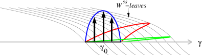
Figure 2: Geometry of folding in relation to the $W^{ss}$-foliation. Shown are the kicked image of a segment $\gamma_{0}$ and two of its subsequent images under $\Phi_{np}$ , $p={\rm Per}(\gamma)$.

We now examine the action of the kick map $\kappa$ in relation to the $W^{ss}$-foliation. Fig. 2 is analogous to Fig. 1; it shows the image of a segment $\gamma_{0}$ of $\gamma$ under $F_{T}=\Phi_{T}\circ\kappa$. For illustration purposes, we assume $\gamma_{0}$ is kicked upward with its end points held fixed, and assume $T=np$ for some $n\in{\mathbb{Z}}^{+}$ (otherwise the picture is shifted to another part of $\gamma$ but is qualitatively similar). Since $\Phi_{np}$ leaves each $W^{ss}$-manifold invariant, we may imagine that during relaxation, the flow “slides” each point of the curve $\kappa(\gamma_{0})$ back toward $\gamma$ along $W^{ss}$-manifolds. In the situation depicted, the effect of the folding is evident.

Fig. 2 gives considerable insight into what types of kicks are conducive to the formation of strange attractors. Kicks along $W^{ss}$-manifolds or in directions roughly parallel to the $W^{ss}$-manifolds will not produce strange attractors, nor will kicks that essentially carry one $W^{ss}$-manifold to another. What causes the stretching and folding is the variation in how far points $x\in\gamma$ are moved by $\kappa$ as measured in the direction transverse to the $W^{ss}$-manifolds. In the simple model of Eq. (7), because of the linearity of the unforced equation, $W^{ss}$-manifolds are straight lines with slope $~{}-\lambda/\sigma$ in $(\theta,y)$-coordinates. Variation in the sense above is created by any non-constant $H$; the larger the ratio $\frac{\sigma}{\lambda}A$, the greater this variation.

The notion of “phases” in Sect. 1.1 is defined precisely by the partition of neighborhoods of $\gamma$ into $W^{ss}$-manifolds or isochrons (two names used by different communities for the same object), i.e., we view $x\in{\rm Basin}(\gamma)$ as having the same phase as $y\in\gamma$ if $x\in W^{ss}(y)$. The ideas in the last paragraph are in the same spirit as the phase transition curves introduced by Winfree [38, 11, 9]. They were discovered independently in the rigorous work of Wang and Young, who proved, under suitable geometric conditions on phase variations, the existence of strange attractors having many of the properties commonly associated with chaos [34, 37]. These ideas have since been applied to various situations; rigorous results include [35, 36, 23, 30, 33] and [5], and numerical results indicate the occurrence of shear-induced chaos in broader dynamical settings [18, 20, 17].

1.4 Summary and comparisons

Sects. 1.1 and 1.3 outlined two seemingly distinct approaches to the analysis of phase response. These approaches are in fact closely related: In Sect. 1.1, perturbations are assumed to be small, which geometrically means one can approximate $W^{ss}(y)$ by its linearization around $\gamma$ . The procedure of phase reduction then amounts to viewing the perturbation as a sequence of infinitesimal kicks, projecting the kicked trajectory back to $\gamma$ along $W^{ss}$-leaves following each kick. The analysis sketched in Sect. 1.3 is a more global version of the same idea: here the perturbed orbit is allowed to wander farther away from $\gamma$, and one takes into consideration the geometry (or curvature) of the $W^{ss}$-manifolds in relation to the kick in assessing its impact.

A notable difference between full-model analyses and phase reductions is that the latter rule out a priori any possibility of chaotic behavior. As explained in Sect. 1.3, in the full model, fairly innocuous kicks applied “the right way” can lead to positive Lyapunov exponents for large sets of initial conditions. This cannot be captured by the infinitesimal PRC, for flows in one spatial dimension are never chaotic.

With regard to practicalities, full model analyses are, needless to say, more costly. While our aim here has been to raise awareness of the issues discussed in Sects. 1.2 and 1.3, it is not our intention to advocate that one necessarily starts by computing $W^{ss}$-manifolds (even though they are computable in many situations). In many cases, by far the most direct way to get a quick idea of whether shear-induced chaos is present is to look at $F_{T}$-images of $\gamma$ (recall that $F_{T}=\Phi_{T}\circ\kappa$ is the composite map obtained by first kicking then following the unperturbed dynamics for time $T$) and see if folds develop. See Section 3.

2 A neuron model

In Sects. 3–5, a few concrete scenarios will be presented to illustrate how and why the infinitesimal PRC may give incorrect predictions. The model we use is taken from neuroscience; it is the Morris-Lecar (ML) model of neuron dynamics. A brief introduction of the ML model and some relevant information is given below to provide context for readers not familiar with the subject. We remark that perturbation methods and the infinitesimal PRC in particular are widely used in neuroscience, both in the study of single neuron dynamics (see e.g. [9]) and in the analysis of neuronal networks modeled as systems of coupled phase oscillators (see e.g. [16]).

The Morris-Lecar (ML) model

The dominant mode of communication between neurons is via the generation and transmission of action potentials, or “spikes” [4]. Neurons accomplish this through the coordinated activity of voltage-sensitive ion channels in the cell membrane, which open and close in specific ways in response to changes in membrane voltage. The ML model is a simple model of this spike-generation process for a single neuron. It has the form

$$\begin{array}[]{rcl}C_{m}~{}\dot{v}&=&I(t)-g_{\rm leak}\cdot(v-v_{\rm leak})-g_{K}~{}w\cdot(v-v_{K})-g_{\rm Ca}~{}m_{\infty}(v)\cdot(v-v_{\rm Ca})\\[8.61108pt] \dot{w}&=&\phi\cdot\big{(}w_{\infty}(v)-w\big{)}/\tau_{w}(v)~{}.\end{array}$$ (8)

The variable $v$ is the membrane voltage; the first equation expresses Kirchoff’s current law across the cell membrane, with $I(t)$ representing a stimulus in the form of an incoming current. The variable $w$ is a gating variable: it describes the fraction of membrane ion channels that are open at any time. Real-life neurons typically have multiple kinds of ion channels; in more realistic models like Hodgkin-Huxley, these are tracked by separate gating variables. The ML model is simplified in that there is just one effective gating variable. The forms and meanings of the auxiliary functions $w_{\infty}$ , $\tau_{w}$ , $m_{\infty}$ and other parameters in (8) are given in the Appendix. For more information we refer the reader to [9].

The ML model has a very rich bifurcation structure. Roughly speaking, by varying a constant current $I(t)\equiv I_{0}$ , one observes, in different parameter regions, dynamical regimes corresponding to sinks, limit cycles, and Hopf, saddle-node and homoclinic bifurcations, as well as combinations of the above. These scenarios together with their neuroscience interpretations are discussed in detail in [9]. We will use two of these scenarios for illustration; relevant features of these regimes are reviewed as needed in the sections to follow.

Oscillators in neuronal dynamics

When a sufficiently large DC current is injected into a neuron, either artificially or through the action of neurotransmitters, a typical neuron will begin to spike regularly. In such situations, one can view the neuron as an oscillator. For example, in Eq. (8), if we apply a constant driving current $I(t)\equiv I_{0}$ and slowly increase $I_{0}$ from 0 to a large value, the ML neuron will switch from quiescent to spiking at regular intervals, the latter corresponding to the emergence of a limit cycle. More generally, if a neuron is operating in a “mean-driven” regime, in which the stimulus it receives consists of a large DC component plus a (weaker) fluctuating AC component, one can view the AC component of the stimulus as a perturbation of the oscillator [9].

Relevant properties

The crudest statistic associated with a spiking neuron it is firing rate, which translates into the frequency of the neural oscillator. Sometimes one is also interested in more refined properties of spike trains and even the precise timing of spikes.

A neuron or a network of neurons receiving a stimulus is said to be reliable if its response does not vary significantly upon repeated presentations of the same stimulus. Reliability is of interest because it constrains a neuron’s (or network’s) ability to encode information via temporal patterns of spikes. Mathematically, a stimulus-driven system can be viewed as a non-autonomous dynamical system of the form $\dot{x}=f(x,I(t))~{},$ where $I(t)$ represents the stimulus. The question of spike-time reliability, then, boils down to the following: Given a specific signal $\big{(}I(t):t\in[0,\infty)\big{)}$ , does the response $x(t)$ depend (modulo transients) in an essential way on $x(0)$, the condition of the system at the onset of the stimulus? If the answer is negative, the system is reliable. Otherwise, it is unreliable.

The relevant dynamical quantity here is $\Lambda_{\max}$, the largest Lyapunov exponent of the system : If $\Lambda_{\max}<0$, then the system is reliable, whereas $\Lambda_{\max}>0$ leads to unreliability. Heuristically, this is because $\Lambda_{\max}<0$ leads to phase space contraction, so that the effects of initial conditions are quickly forgotten, whereas $\Lambda_{\max}>0$ leads the system to amplify small differences in initial states. The reasoning can be made more precise via the theory of random dynamical systems and random attractors; see [20, 21, 22] for details.

3 Chaotic response to periodic kicking

In this section, we show numerically that shear-induced chaos occurs in the “homoclinic regime” of the ML model (see below), leading to a lack of reliability. As noted in Sect. 1.4, such a possibility is ruled out a priori by the infinitesimal PRC.

3.1 Geometry of the “homoclinic regime”

We view Eq. (8) with $I(t)\equiv I_{0}$ for some fixed $I_{0}$ as the unperturbed system, and apply to it a forcing in the $v$-variable (forcing the system in $w$ has no physical meaning).

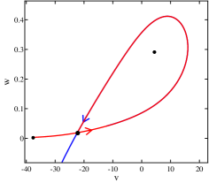
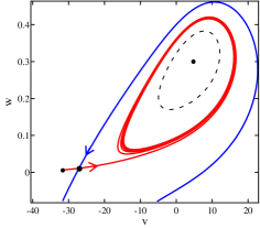
(a) At the moment of a homoclinic bifurcation, $I_{0}\approx 35$		(b) The “homoclinic regime” at $I_{0}=39.5$

Figure 3: A homoclinic bifurcation and the “homoclinic regime.” In this parameter regime, the system has 3 fixed points (shown as black dots), the middle one being a saddle for a broad range of $I_{0}$ . Panel (a) shows a homoclinic loop anchored at the saddle, with a source on the right and a sink on the left. As $I_{0}$ increases, the homoclinic loop breaks apart and a limit cycle emerges. Panel (b) shows the phase portrait at the parameter regime we use, which is well past the homoclinic bifurcation. In addition to the homoclinic bifurcation shown in (a), a (subcritical) Hopf bifurcation has occurred, leading the fixed point on the right to become a sink surrounded by an unstable periodic orbit / cycle (dashed curve).

At $I_{0}=I_{\rm crit}\approx 35$, for suitable choices of parameters (details of which are given in the Appendix), Eq. (8) has a homoclinic loop, i.e. there is a saddle fixed point $p$ one branch of whose stable and unstable manifolds coincide (see Fig. 3(a)). To the left of $p$ lies a sink, which attracts the left branch of the unstable manifold; and there is a source inside the loop.

For $I_{0}>I_{\rm crit}$, the homoclinic loop is broken, with the unstable manifold “inside” the stable manifold. Fig. 3(b) shows the phase flow at $I_{0}=39.5$. The unstable manifold wraps around a newly emerged limit cycle, which will be our $\gamma$. Notice also the other dynamical structures: the saddle $p$, its stable and unstable manifolds and the sink to the left, plus a new sink and unstable cycle (indicated by the dashed loop) that emerged from the original source via a Hopf bifurcation (the latter occurs around $I_{0}\approx 36.3$). In the rest of this section, $I_{0}$ will be taken around $39.5$, and the unforced flow is qualitatively similar to that in Fig. 3(b).

We consider periodic kicks applied to such a regime, i.e., in Eq. (8) we take as input $I(t)=I_{0}+A\sum_{k}\delta(t-kT)~{},$ where $|A|$ is the kick amplitude and $T$ the kick period. Geometrically, this kick corresponds to shifting simultaneously all phase points by $A$ (which can be positive or negative) in the horizontal direction.

If $|A|$ is sufficiently large, some very obvious things can happen: For example, a large kick to the left can easily drive points on $\gamma$ to the left of the stable manifold of the saddle; these points will then head for the sink on the left and possibly never return. Another possibility is to drive points into the basin of attraction of the sink inside the unstable cycle. We will show in the next subsection that something more subtle can happen even with small to medium kicks which do not drive points outside of the basin of $\gamma$.

3.2 Shear-induced chaos

We will proceed in three stages: First, we discuss – on a theoretical level – the dynamical mechanism responsible for shear production in the regimes of interest. Then we perform some relatively quick, exploratory numerical simulations to check that this shear is sufficiently strong, and to identify suitable parameters. Finally, we confirm the presence of shear-induced chaos via careful computations of Lyapunov exponents.

What is the mechanism that produces shear in the present setting?

Take $A<0$, so that the kick $\kappa$ moves the limit cycle $\gamma$ to the left of itself. This pushes about half of $\gamma$ inside the unstable cycle, and half of it outside and to the left. Now suppose we go through a period of relaxation, i.e., we apply the ML flow $\Phi_{t}$, no kicks. As points come down the left side of $\gamma$, those that are closer to the stable manifold of the saddle $p$ are likely to follow it longer; consequently they will come closer to $p$. (We assume the kick is small enough that no point gets kicked to the other side of the stable manifold.) It is easy to see that the closer an orbit comes to a saddle fixed point, the longer it remains in its vicinity – certainly longer than orbits that are, for example, inside the unstable cycle. The differential in “time spent near $p$”, if strong enough, may lead to a fold in the $(\Phi_{t}\circ\kappa)$-image of $\gamma$.

The argument above can be made rigorous. Similar ideas have been used in rigorous work [1, 33]. But the reasoning is qualitative: while it shows that some amount of shear is present, it does not tell us whether it is sufficient to cause chaos.

$t=0$	$t=5$	$t=10$
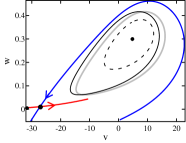
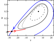
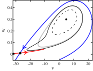
$t=15$	$t=20$	$t=25$

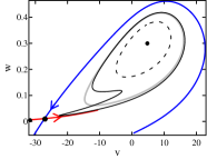
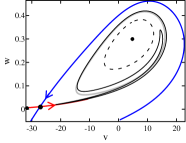
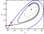
Figure 4: Shear-induced folding in the Morris-Lecar model. Here, the stable cycle is given one kick with $A=-2$, then allowed to relax back to the cycle. The limit cycle $\gamma$ is shown in gray; also shown are the 3 fixed points (dots), the stable and unstable manifolds of the saddle, and the unstable cycle (dashed curve).

Simulations to detect shear-induced chaos

As noted in Sect. 1.4, by far the most direct way to detect the presence of shear-induced chaos is to plot the images of $\kappa(\gamma)$ under the unperturbed flow, and to see if folds develop in time. A sample “movie” is shown in Fig. 4. As one can see, by $t=10$, a “tail” has developed: some points in this tail are evidently stuck near the saddle, while some other points, evidently $\Phi_{t}$-images of points kicked inside the unstable cycle, have remained inside, and at $t=10$ they are beginning to gain on points in the tail in terms of their angular position (or phase) around $\gamma$. At $t=15$, these points have overtaken those in the tail, and the difference is further exaggerated in the last two frames. One would conclude that for the parameters shown, the system very likely has shear-induced chaos.

Because this step can be done quickly for the ML model, we use it to locate parameters with the desired properties. The kick size used in Fig. 4 is $A=-2$, which is quite reasonable physiologically: it takes at least 10-15 kicks of this size to push a neuron over threshold. Fig. 4 also tells us that it takes on the order of 15 units of time for the fold to begin to form, so that for a periodically-kicked system to produce chaos, the kick period should probably be upwards of 20 units of time. (Kicks delivered too frequently may also drive points to the left of the stable manifold of $p$; once that happens, it will end up near the left sink.)

Fig. 5 shows the strange attractor that results from a periodically-kicked regime.

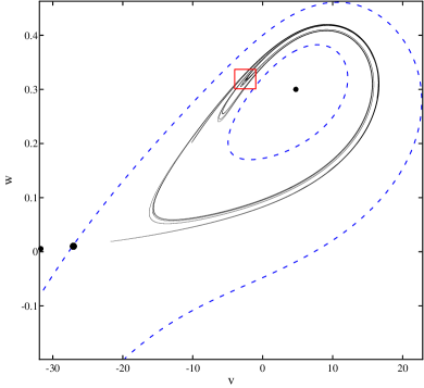
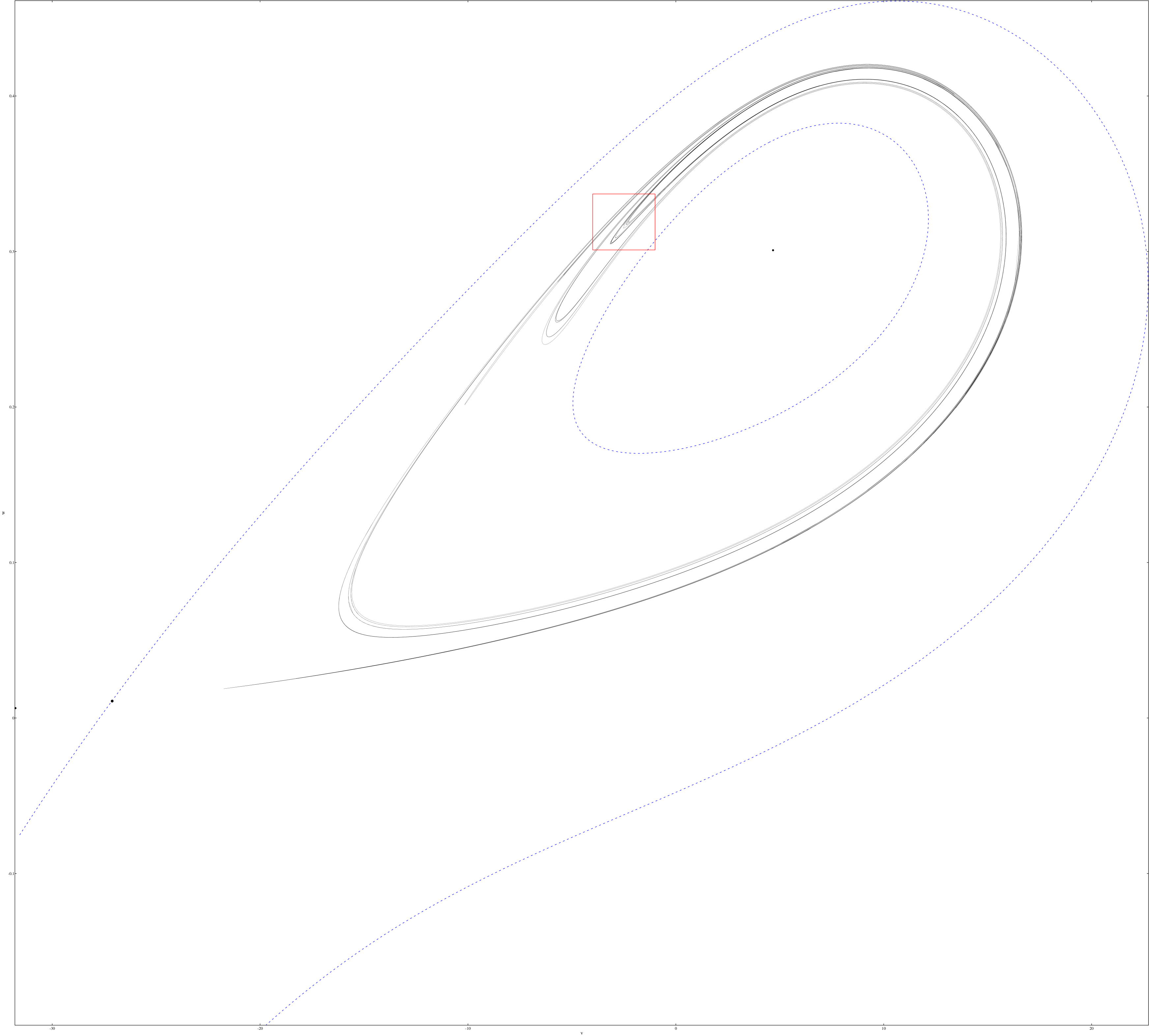
Figure 5: A strange attractor created by shear-induced chaos. The dashed curves show the basin boundary of the limit cycle $\gamma$ . Here $A=-2,T=27$.

Lyapunov exponents

Let us now explore the chaotic behavior more systematically. Fig. 6(a) shows the largest Lyapunov exponent $\Lambda_{\max}$ as a function of the kick period $T$, for a variety of kick amplitudes. More precisely, given a phase point $(v_{0},w_{0})$ and a tangent vector $\eta_{0}$, we let $\eta(t)$ be the solution of the variational equation for the kicked system, and define

$$\Lambda_{\max}(v_{0},w_{0};\eta_{0})=\lim_{t\to\infty}\frac{1}{t}\log|\eta(t)|\ .$$

It is a standard fact that for each $(v_{0},w_{0})$, $\Lambda_{\max}(v_{0},w_{0};\eta_{0})$ is equal to the largest Lyapunov exponent except for $\eta_{0}$ in a lower dimensional subspace (see, e.g., [6]). In many (but not all) of the cases considered, this number is independent of the choice of $(v_{0},w_{0})$.

For small $A$, the exponents are predominantly negative, just as we would expect: the dynamical landscape is characterized by sinks and saddles. As $A$ increases, the tendency to form positive exponents becomes greater, so that for $A=-2$ and sufficiently large $T$, most exponents sampled are positive, confirming the strong form of (sustained and observable) chaos discussed in Sect. 1.3. Note, however, that this is only a tendency: the fluctuations seen in the Lyapunov exponents as we vary $T$ are likely real, and reflect the competition between the “horseshoes and sinks” and “strange attractors” scenarios.

As explained in Sect. 2, Lyapunov exponents are useful as probes of neuronal reliability. This is illustrated in Fig. 6(b). The left panel there shows the response of a system with $\Lambda_{\max}<0$: clearly, after some transients, the response of the system is the same across all the trials. In the right panel, we have $\Lambda_{\max}>0$, and the resulting spike times show significant variability across trials. Moreover, this variability will persist in time due to the presence of sustained chaos.

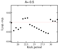
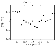
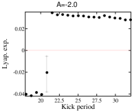
(a) Lyapunov exponents

Reliable ($\Lambda_{\max}\approx-0.02$)	Unreliable ($\Lambda_{\max}\approx 0.035$)

(b) Spike times over repeated trials

Figure 6: Lyapunov exponents and reliability of the ML system. In (a), we plot the Lyapunov exponents. In (b), we plot spike times generated by reliable (left) and unreliable (right) systems over repeated trials, with random initial conditions sampled from a neighborhood of $\gamma$. The exponents in (a) are computed as follows: For each choice of kick amplitude and kick period, 6 random initial conditions are used to estimate exponents via long-time simulations. The max and min are treated as outliers and discarded; the remaining are used to form error bars. The dot marks the median.

We finish with the following two remarks: (1) While we have focused on the periodically kicked case, similar-sized kicks that arrive at random times that are, on average, sufficiently far apart will lead to time-dependent strange attractors for much the same reasons as we have discussed. We will not pursue this here, but refer the reader to [18, 20]. (2) Notice that the saddle $p$, which is the root cause of the chaos in the kicked system in the sense that it is responsible for scrambling the order (or phases) of the points on $\kappa(\gamma)$, does not lie that close to the limit cycle. Not only would phase reduction methods miss this effect, but the PRC will offer no hint at all that any breakdown has occurred.

4 Firing rates and interspike intervals

We demonstrate in this section that, as asserted in item (2) of Sect. 1.2, “sticky” sets in the boundary of ${\rm Basin}(\gamma)$ can lead to discrepancies between the dynamical behavior of the full model and that deduced from the infinitesimal PRC. Specifically, we will present numerical data to show in the example considered that firing rates for the full model are significantly lower and interspike intervals (ISIs) are longer and more spread out than those predicted by the PRC.

For the unperturbed flow, we continue to use the example from the last section, with the same parameters. Recall that this system is in the “homoclinic regime” of ML, with a limit cycle we call $\gamma$. Shown in dashed lines in Fig. 5 are part of $\partial({\rm Basin}(\gamma))$, the boundary of the basin of attraction of $\gamma$: one component is the stable manifold $W^{s}$ of $p$; the other is a repelling periodic orbit. As discussed in Sect. 3.2, all orbits close enough to $W^{s}$ will follow it to $p$ and remain there for some time before moving away, $\{p\}$ is a candidate “sticky set” in this example. The repelling periodic orbit is in some sense also a sticky set, especially if the expansion away from the orbit is weak (it is, since it has just emerged from a Hopf bifurcation). Indeed orbits that come close to it may cross over to the other side and get pushed toward the sink.

Instead of periodic forcing, here we drive the oscillator with white noise in addition to the steady current $I_{0}$, i.e., we let $I(t)=I_{0}+\beta\cdot C_{m}\cdot\dot{W}~{}$, and consider the random dynamical system that results from looking at one realization of $\dot{W}$ at a time. For the phase reduced model, it is natural to regard the system as producing one spike as it passes through a marked point on the cycle. For the full ML model, it is necessary to fix an artificial definition of what it means for the system to “spike”: we define a reset to be when the voltage falls below -10, and say the neuron “spikes” when (after a reset) the voltage rises above +12.5. See Fig. 5 for how this corresponds to the location of the limit cycle.

Comparison of firing rates. The results are shown in Fig. 7(a). Plotted are firing rates as a function of the drive amplitude $\beta$ for three different systems: (i) the full ML system; (ii) the firing rate of the phase reduction, computed empirically; and (iii) the firing rate of the phase reduction as computed by the perturbative formula (5) of Ly and Ermentrout. We plot both (ii) and (iii) because Eq. (5) is itself an approximate result based on the phase reduction (4), valid only for small $\beta$. As one would expect, for smaller forcing amplitudes ($<0.1$), all three agree. As $\beta$ increases, the perturbative formula tracks the empirical firing rate of the phase reduction fairly well, but neither of these PRC-based predictions capture the dramatic drop in firing rate of the full system occurring around $\beta=0.2$. Simulations (an example of which is shown in Fig. 7(b)) show that the precipitous drop in firing rate in this case has to do with trajectories spending more time near the saddle $p$.

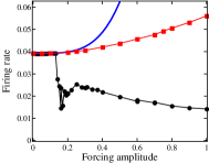
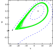
(a)	(b)

Figure 7: Firing rate statistics of the stochastically-forced ML model. In (a), we compare of firing rates for the full ML system and its phase reduction driven by white noise. Black dots: Full ML. Red squares: Empirical phase reduction firing rate. Solid blue curve: Perturbative formula for PRC firing rate (see Eq. (5)). Panel (b) shows a long sample path for $\beta=0.2$ .

Comparison of ISI distributions. Fig. 8 shows the numerically computed ISI distributions for the full ML model and for the phase reduction (4). For small noise, we see the full ML system and phase reduction agree fairly well: the ISI distribution is concentrated around the period of the cycle (about 25.2), and the shape is roughly gaussian. As noise amplitude increases, we see in the full ML system (i) a broadening of the ISI distribution, and (ii) an overall shift toward larger ISIs. Neither of these effects are captured by the PRC, as they involve structures a finite distance away from $\gamma$ .

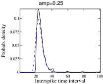
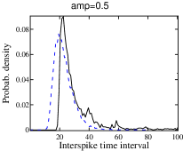
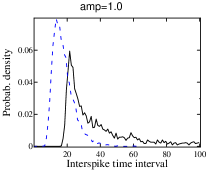
Figure 8: interspike interval (ISI) distributions for various $\beta$. Solid black lines: ISI histograms for the full ML system. Dashed blue lines: ISI histograms for the phase reduction (4).

Finally, to compare the tails of the ISI distributions, here are the fraction of ISIs greater than $2\times\mbox{(cycle period)}$:

$\beta$	Full ML	PRC
0.25	0.0225	0.0003
0.5	0.127	0.0032
1.0	0.322	0.0013

Notice that the PRC systematically under-predicts the probability of a long interspike interval, consistent with the “trapping” effect of nearby invariant structures.

5 Altered spiking patterns in bistable systems

In this last section, we present a simple example in which the perturbation takes an orbit outside of ${\rm Basin}(\gamma)$, the scenario described in item (1) of Sect. 1.2. It is no surprise that PRC predictions would break down here. Perhaps the lesson to take away from this example is that even a weak drive can lead to spike patterns that are nontrivially different.

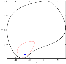
Figure 9: ML phase portrait in the Hopf regime. Shown are a limit cycle surrounding an unstable cycle, which in turn surrounds a sink. Here, $I_{0}=90$, corresponding to an unforced period of about 102 ms.

For the unperturbed system, we consider here parameters of ML that put it in a “Hopf regime”, with $I_{0}\approx 90$. Precise parameters used are given in the Appendix, and some relevant dynamical structures are shown in Fig. 9. In this regime, the system has a limit cycle, which we call $\gamma$. Each time an orbit passes near the right-most point of $\gamma$, we think of it as producing a “spike”. Notice that this system is bistable: inside $\gamma$ there is a sink, the basin of attraction of which is separated from the basin of $\gamma$ by a repelling periodic orbit (from a Hopf bifurcation). This repelling periodic orbit is very close to $\gamma$, but since it is a positive distance away, it will not show up in PRC considerations.

Full ML, $\beta=0.2$

Full ML, $\beta=0.4$

PRC, $\beta=0.4$

$t$

Figure 10: Voltage traces for the ML system in Hopf regime. The top two panels show simulation using the full ML model with the indicated level of stochastic forcing. The bottom panel shows the PRC using $\beta=0.4$. Here, $I_{0}=90$.

We now consider perturbations to the ML model above. As in Sect. 4, we again use a white-noise perturbation, i.e., $I(t)=I_{0}+\beta\cdot C_{m}\cdot\dot{W}~{}.$ Fig. 10 shows the resulting voltage traces of the full model and PRC predictions (computed at $I_{0}=90$). The top panel shows the full ML simulation with $\beta=0.2$ (a relatively weak forcing), starting the trajectory on $\gamma$ . Since the basin of the sink, i.e., the unstable periodic orbit shown in Fig. 9, is so close to the limit cycle $\gamma$, a trajectory following $\gamma$ can easily get pushed into the basin, and then attracted to the sink. This can happen even with very small $\beta$. The sink itself, however, is a little farther from the boundary of its basin, so it is more difficult for a trajectory near the sink to escape under weak $\beta$. This is why for weak noise like $\beta=0.2$, it is easy to observe a transition from $\gamma$ to the sink, but not easy to see transition in the reverse direction.

For $\beta$ a little larger, e.g., $\beta=0.4$, the trajectory jumps back and forth more readily: it alternately follows (roughly) the limit cycle $\gamma$ and stays near the sink, switching between the “spiking” and “quiescent” modes at somewhat random times. Not surprisingly, in the phase-reduced model (bottom panel), these perturbations do not have a significant impact, and the spiking ranges from completely regular to slightly irregular in the second case due to the effect of the noise. PRC voltage traces for $\beta=0.2$ (not shown) are quite similar.

Finally, we note that in this bistable situation, a neuron can exhibit substantial sub-threshold activity. The PRC underestimates the extent of such activity.

Conclusions

This paper compares two ways of evaluating an oscillator’s response to perturbations: phase reductions versus analysis of the full model. We have found that the infinitesimal PRC, which has the virtue of being both straightforward to execute and reducing model dimensionality, produces regular oscillatory behavior even when the full model does not. Specifically, we presented examples from the Morris-Lecar neuron model to show that

1. Periodic kicking of the ML system can lead to unreliable response in the full model via the mechanism of shear-induced chaos, contrary to PRC predictions.

2. When stochastically driven, stickiness of nearby invariant structures can lead to lower firing rates and longer ISIs compared to PRC predictions.

3. The forcing need not be strong to bring about serious discrepancies in firing patterns between full and phase-reduced models.

Moreover, in all the situations examined, the phase reduction itself offers no hint that any breakdown has occurred.

In terms of neuronal response, our results have the following interpretation: Under certain conditions, PRCs may overestimate spike-time reliability and firing rates; they may also underestimate the mean and variance in interspike intervals, and have a tendency to downplay sub-threshold activity. Caution needs to be exercised when interpreting results that come from phase reduction arguments, especially for systems near bifurcation points.

While we have focused on the ML model for illustration, the geometric ideas we used are quite general, and we expect similar phenomena to occur in a variety of settings that involve rhythms and oscillations.

Finally, given that pure phase reductions cannot always capture the behavior of high dimensional nonlinear oscillators, are there alternative methods that give better characterizations? One classical technique, which has seen relatively little application in biological modeling, is that of moving-frame coordinates for the analysis of periodic orbits. This is nicely described in Hale [15] and recently advocated in a neuroscience context by Medvedev [26]. In essence this offers a coordinate transformation to a phase-amplitude system that allows one to track the evolution of distance from the cycle as well as phase on the cycle. We are currently developing this approach and using it to better understand the three points listed above. This, and a framework for understanding the dynamics of weakly coupled phase-amplitude models, will be presented elsewhere.

Acknowledgements.

KKL is supported in part by the US National Science Foundation (NSF) through grant DMS-0907927. KCAW and SC acknowledge support from the CMMB/MBI partnership for multiscale mathematical modelling in systems biology - United States Partnering Award; BB/G530484/1 Biotechnology and Biological Sciences Research Council (BBSRC). LSY is supported in part by NSF grant DMS-1101594.

Appendix. Morris-Lecar model details

Here we briefly summarize the details of the ML model used in this paper. The interested reader is referred to [8, 9] for more details.

Recall the ML equations

$$\begin{array}[]{rcl}C_{m}~{}\dot{v}&=&I(t)-g_{\rm leak}\cdot(v-v_{\rm leak})-g_{K}~{}w\cdot(v-v_{K})-g_{\rm Ca}~{}m_{\infty}(v)\cdot(v-v_{\rm Ca})\\[8.61108pt] \dot{w}&=&\phi\cdot\big{(}w_{\infty}(v)-w\big{)}/\tau_{w}(v)~{}.\end{array}$$

As explained in Sect. 2, the ML model tracks the membrane voltage $v$ and a gating variable $w$. The constant $C_{m}$ is the membrane capacitance, $\phi$ a timescale paramter, and $I(t)$ an injected current.

Spike generation depends crucially on the presence of voltage-sensitive ion channels that are permeable only to specific types of ions. The ML equations include just two ionic currents, here denoted calcium and potassium. The voltage response of ion channels is governed by the $w$-equation and the auxiliary functions $w_{\infty}$ , $\tau_{w}$ , and $m_{\infty}$ , which have the form

$$\begin{array}[]{rcl}m_{\infty}(v)&=&\frac{1}{2}\big{[}1+\tanh\big{(}(v-v_{1})/v_{2}\big{)}\big{]}~{},\\[6.45831pt] \tau_{w}(v)&=&1/\cosh\big{(}(v-v_{3})/(2v_{4})\big{)}~{},\\[6.45831pt] w_{\infty}(v)&=&\frac{1}{2}\big{[}1+\tanh\big{(}(v-v_{3})/v_{4}\big{)}\big{]}~{}.\end{array}$$

The function $m_{\infty}(v)$ models the action of the relatively fast calcium ion channels; $v_{\rm Ca}$ is the “reversal” (bias) potential for the calcium current and $g_{\rm Ca}$ the corresponding conductance. The gating variable $w$ and the functions $\tau_{w}(v)$ and $w_{\infty}(v)$ model the dynamics of slower-acting potassium channels, with its own reversal potential $v_{\rm K}$ and conductance $g_{\rm K}$ . The constants $v_{\rm leak}$ and $g_{\rm leak}$ characterize the “leakage” current that is present even when the neuron is in a “quiescent” state. The forms of $m_{\infty}$ , $\tau_{w}$ , and $w_{\infty}$ (as well as the values of the $v_{i}$) can be obtained by fitting data, or reduction from more biophysically-faithful models of Hodgkin-Huxley type (see, e.g., [9]).

The precise parameter values used in this paper are summarized in Table 1. These are obtained from [9].

Parameter	Homoclinic regime	Hopf regime
$I_{0}$	39.5	90
$C_{m}$	20.0	20.0
$g_{\rm Ca}$	4.0	4.4
$g_{K}$	8.0	8.0
$g_{\rm leak}$	2.0	2.0
$v_{K}$	-84.0	-84.0
$v_{\rm leak}$	-60.0	-60.0
$v_{\rm Ca}$	120.0	120.0
$\phi$	0.23	0.04
$v_{1}$	-1.2	-1.2
$v_{2}$	18.0	18.0
$v_{3}$	12.0	2.0
$v_{4}$	17.4	30.0

Table 1: ML parameter values used in this paper.

References

- [1] V. S. Afraimovich and L. P. Shilnikov, “The ring principle in problems of interaction between two self-oscillating systems,” J. Appl. Math. Mech. 41 (1977) pp. 618–627
- [2] E. Brown, J. Moehlis, and P. Holmes, “On the phase reduction and response dynamics of neural oscillator populations,” Neural Computat. 16 (2004) pp. 673–715
- [3] A. H. Cohen, S. Rossignol, and S. Grillner, eds., Neural Control of Rhythmic Movements in Vertebrates, John Wiley, 1988
- [4] P. Dayan and L. Abbott, Theoretical Neuroscience: Computational and Mathematical Modeling of Neural Systems, MIT Press, 2001
- [5] R. E. L. Deville, N. Sri Namachchivaya, Z. Rapti, “Stability of a stochastic two-dimensional non-Hamiltonian system,” SIAM J. Appl. Math., to appear (2011)
- [6] J.-P. Eckmann and D. Ruelle, “Ergodic theory of chaos and strange attractors,” Rev. Mod. Phys. 57 (1985) pp. 617–656
- [7] G. B. Ermentrout and N. Kopell, “Multiple pulse interactions and averaging in coupled neural oscillators,” J. Math. Biol. 29 (1991) pp. 195–217
- [8] G. B. Ermentrout and J. Rinzel, “Analysis of neural excitability and oscillations,” in Methods in Neuronal Modeling: From Synapses to Networks, C. Koch and I. Segev, eds., Bradford Books (1991)
- [9] G. B. Ermentrout and D. H. Terman, Mathematical Foundations of Neuroscience, Interdisciplinary Applied Mathematics 35, Springer (2010)
- [10] L. Glass, M. R. Guevara, J. Belair, and A. Shrier, “Global bifurcations of a periodically forced biological oscillator,” Phys. Rev. A 29 (1984) pp. 1348–1357
- [11] L. Glass and M. C. Mackey, From Clocks to Chaos: The Rhythms of Life, Princeton University Press (1988)
- [12] M. Golubitsky, I. Stewart, P. L. Buono, and J. J. Collins, “Symmetry in locomotor central pattern generators and animal gaits,” Nature 401 (1999) pp. 693–695
- [13] J. Guckenheimer, “Isochrons and phaseless sets,” J. Theor. Biol. 1 (1974) pp. 259–273
- [14] J. Guckenheimer and P. Holmes, Nonlinear Oscillations, Dynamical Systems, and Bifurcations of Vector Fields, Springer-Verlag (1983)
- [15] J. K. Hale, Ordinary Differential Equations, John Wiley and Sons, 1969
- [16] F. C. Hoppensteadt and E. M. Izhikevich, Weakly Connected Neural Networks, Springer-Verlag, 1997
- [17] K. K. Lin, “Entrainment and chaos in a pulse-driven Hodgkin-Huxley oscillator,” SIAM J. Applied Dyn. Sys. 5 (2006) pp. 179–204
- [18] K. K. Lin and L.-S. Young, “Shear-induced chaos,” Nonlinearity 21 (2008) pp. 899–922
- [19] K. K. Lin and L.-S. Young, “Dynamics of periodically-kicked oscillators,” J. Fixed Point Theory & Appl. 7 (2010) pp. 291–312
- [20] K. K. Lin, E. Shea-Brown, and L.-S. Young, “Reliability of coupled oscillators,” J. Nonlin. Sci. 19 (2009) pp. 630–657
- [21] K. K. Lin, E. Shea-Brown, and L.-S. Young, “Reliability of layered neural oscillator networks,” Commun. Math. Sci. 7 (2009) pp. 239–247
- [22] K. K. Lin, E. Shea-Brown, and L.-S. Young, “Spike-time reliability of layered neural oscillator networks,” J. Computat. Neurosci. 27 (2009) pp. 135–160
- [23] K. Lu, Q. Wang, and L.-S. Young, “Strange attractors for periodically forced parabolic equations,” preprint
- [24] C. Ly and G. B. Ermentrout, “Analytic approximations of statistical quantities and response of noisy oscillators,” Physica D 240 (2011) pp. 719–731
- [25] R. M. May, “Limit cycles in predator-prey communities,” Science 177 (1972) pp. 900–902
- [26] G. S. Medvedev, “Synchronization of coupled limit cycles,” J. Nonlin. Sci. 21 (2011) pp. 441–464
- [27] R. E. Mirollo and S. H. Strogatz, “Synchronization of pulse-coupled biological oscillators,” SIAM J. Applied Math. 50 (1990) pp. 1645–1662
- [28] T. I. Netoff, C. D. Acker, J. C. Bettencourt, and J. A. White, “Beyond two-cell networks: experimental measurement of neuronal responses to multiple synaptic inputs,” J. Computat. Neurosc. 18 (2005) pp. 287–295
- [29] S. A. Oprisan, V. Thirumalai, C. C. Canavier, “Dynamics from a time series: Can we extract the phase resetting curve from a time series?” Biophys. J. 84 (2003) pp. 2919–2928
- [30] W. Ott and M. Stenlund, “From limit cycles to strange attractors,” Commun. Math. Phys. 296 (2010) pp. 215–249
- [31] A. Pikovsky, M. Rosenblum, and J. Kurths, Synchronization: A Universal Concept in Nonlinear Sciences, Cambridge University Press (2001)
- [32] R. Thul, T. C. Bellamy, H. L. Roderick, M. D. Bootman, and S. Coombes, “Calcium oscillations,” in Cellular Oscillatory Mechanisms, M. Maroto and N. Monk, Eds., Advances in Experimental Medicine and Biology, Springer, 2008
- [33] Q. Wang and W. Ott, “Dissipative homoclinic loops of two-dimensional maps and strange attractors with one direction of instability,” Commun. Pure Applied Math., to appear (2011)
- [34] Q. Wang and L.-S. Young, “Strange attractors with one direction of instability,” Comm. Math. Phys. 218 (2001) pp. 1–97
- [35] Q. Wang and L.-S. Young, “From invariant curves to strange attractors,” Comm. Math. Phys. 225 (2002) pp. 275–304
- [36] Q. Wang and L.-S. Young, “Strange attractors in periodically-kicked limit cycles and Hopf bifurcations,” Comm. Math. Phys. 240 (2003) pp. 509–529
- [37] Q. Wang and L.-S. Young, “Toward a theory of rank one attractors,” Annals of Mathematics 167 (2008) pp. 349–480
- [38] A. Winfree, The Geometry of Biological Time, Second Edition, Springer-Verlag (2000)
- [39] L.-S. Young, “What are SRB measures, and which dynamical systems have them?,”J. Statist. Phys. 108 (2002) pp. 733–754
- [40] G. Zaslavsky, “The simplest case of a strange attractor,” Physics Letters 69A (1978) pp. 145–147