Analyzing direct dark matter detection data
with unrejected background events
by the AMIDAS website

Abstract

In this talk I have presented the data analysis results of extracting properties of halo WIMPs: the mass and the (ratios between the) spin–independent and spin–dependent couplings/cross sections on nucleons by the AMIDAS website by taking into account possible unrejected background events in the analyzed data sets. Although non–standard astronomical setup has been used to generate pseudodata sets for our analyses, it has been found that, without prior information/assumption about the local density and velocity distribution of halo Dark Matter, these WIMP properties have been reconstructed with $\sim$ 2% to  $\stackrel{{\scriptstyle\textstyle<}}{{\sim}}$  30% deviations from the input values.

1 Introduction

In order to extract properties of halo WIMPs (Weakly Interacting Massive Particles) by using data from direct Dark Matter detection experiments as model–independently as possible, we have developed a series of data analysis method for reconstructing the one–dimensional WIMP velocity distribution [1] as well as determining the WIMP mass [2], the spin–independent (SI) WIMP coupling on nucleons [3] and the ratios between different WIMP couplings/cross sections [4]. Moreover, in collaboration with the DAMNED (DArk Matter Network Exclusion Diagram) Dark Matter online tool [5], part of the ILIAS Project [6], the “AMIDAS” (A Model–Independent Data Analysis System) website for online simulation/data analysis has also been established [7, 8, 9].

In this article, in order to demonstrate the usefulness and powerfulness as well as the model–independence of the AMIDAS package for direct Dark Matter detection experiments, I will analyze blindly some pseudodata sets generated theoretically for different detector materials and present the reconstructed WIMP properties. This means that I will simply upload these data sets onto the AMIDAS website and follow the instructions to reconstruct different WIMP properties without using any information about the input setup used for generating the analyzed pseudodata. For cases in which some information about WIMPs (e.g., the mass $m_{\chi}$) and/or Galactic halo (e.g., the local Dark Matter density $\rho_{0}$) is required, I will naively use the commonly used/favorite values for the data analyses. Moreover, due to the time limit on preparing the presentation for the CYNGUS 2011 workshop, in Ref. [10] we considered only the case of null background events. In this article, we have taken into account a small fraction of possible unrejected background events in the analyzed data sets [11, 12, 13, 14].

After that I show the blindly reconstructed properties of halo WIMPs in Sec. 2, in Sec. 3 I will reveal the input setup and the background spectrum used for generating the analyzed data and compare the reconstructed results to them. Finally, I conclude in Sec. 4.

2 Reconstructed WIMP properties

In this section, I present the reconstructed WIMP properties analyzed by the AMIDAS website. While in each uploaded file there are exactly 50 data sets, in each data set there are on average 50 recorded events (i.e., 50 measured recoil energies); the exact number of total events is Poisson distributed. For simplicity, the experimental minimal and maximal cut–off energies have been set as 0 and 100 keV for all data sets.

In order to check the effect of using a “wrong” elastic nuclear form factor, two forms have been considered for the SI WIMP–nucleus cross section in our analyses. One is the simple exponential form:

$$F_{\rm ex}^{2}(Q)=e^{-Q/Q_{0}}~{}\!.$$ (1)

Here $Q$ is the recoil energy transferred from the incident WIMP to the target nucleus, $Q_{0}$ is the nuclear coherence energy given by $Q_{0}=1.5/m_{\rm N}R_{0}^{2}$, where $R_{0}=\left[0.3+0.91\left(m_{\rm N}/{\rm GeV}\right)^{1/3}\right]~{}\!{\rm fm}$ is the radius of the nucleus and $m_{\rm N}$ is the mass of the target nucleus. Meanwhile, we used also a more realistic analytic form for the elastic nuclear form factor:

$$F_{\rm SI}^{2}(Q)=\left[\frac{3j_{1}(qR_{1})}{qR_{1}}\right]^{2}e^{-(qs)^{2}}~{}\!.$$ (2)

Here $j_{1}(x)$ is a spherical Bessel function, $q=\sqrt{2m_{\rm N}Q}$ is the transferred 3-momentum, for the effective nuclear radius we use

$$R_{1}=\sqrt{R_{A}^{2}-5s^{2}}$$ (3)

with $R_{A}\simeq 1.2~{}\!A^{1/3}~{}{\rm fm}$ and a nuclear skin thickness $s\simeq 1~{}{\rm fm}$. For the SD WIMP–nucleus cross section, we only used the “thin–shell” nuclear form factor:

$$F_{\rm TS}^{2}(Q) = \left\{\begin{array}[]{l l l}j_{0}^{2}(qR_{1})~{}\!,&{}{}{}{}{}{}{}{}&{\rm for}~{}qR_{1}\leq 2.55~{}{\rm or}~{}qR_{1}\geq 4.5~{}\!,\\ {\rm const.}\simeq 0.047~{}\!,&&{\rm for}~{}2.55\leq qR_{1}\leq 4.5~{}\!.\end{array}\right.$$ (6)

2.1 WIMP mass $m_{\chi}$

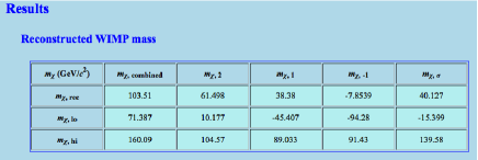
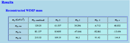
Figure 1: The reconstructed WIMP mass $m_{\chi}$ by means of the method introduced in Ref. [2] with a target combination of ${}^{28}{\rm Si}$ + ${}^{76}{\rm Ge}$ nuclei. Two forms of the elastic nuclear form factor given in Eqs. (1) and (2) have been used in the left and right frames, respectively.

As one of the most important properties of halo WIMPs as well as the basic information for reconstructing other quantities in our model–independent analysis methods, I consider at first the determination of the WIMP mass $m_{\chi}$ by means of the method introduced in Ref. [2].

In Figs. 1 I show the reconstructed WIMP masses and the lower and upper bounds of their 1$\sigma$ statistical uncertainties. The usual target combination of ${}^{28}{\rm Si}$ + ${}^{76}{\rm Ge}$ nuclei has been used for this reconstruction, whereas two analytic forms of the elastic nuclear form factor given in Eqs. (1) and (2) have been used for determining $m_{\chi}$ in the left and right frames, respectively. While $m_{\chi,n}$ with $n=-1$, 1, 2 and $m_{\chi,\sigma}$ have been estimated by Eqs. (34) and (40) of Ref. [2], respectively, $m_{\chi,{\rm combined}}$ has been estimated by the $\chi^{2}$–fitting defined in Eq. (51) of Ref. [2], which combines the estimators for $m_{\chi,n}$ and $m_{\chi,\sigma}$ with each other. The reconstructed WIMP mass $m_{\chi,{\rm combined}}$ as well as $m_{\chi,n}$ and $m_{\chi,\sigma}$ shown here have been corrected by the iterative $Q_{\rm max}$–matching procedure described in Ref. [2].

It can be found here that, although all single estimators ($m_{\chi,n}$ with $n=-1$, 1, 2 and $m_{\chi,\sigma}$) give generally a (relatively lighter) WIMP mass of $\sim 60$ GeV or even lighter and a 1$\sigma$ upper bound of $\sim 140$ GeV, the mean values of the combined (in principle, more reliable) results (second columns) of the reconstructed WIMP mass give $m_{\chi}\sim 115$ GeV with a rough 1$\sigma$ upper (lower) bound of $\sim 190$ (80) GeV, or, equivalently,

$$m_{\chi}\simeq 115_{-35}^{+75}~{}{\rm GeV}~{}\!.$$ (7)

Moreover, the combined results with two different form factors show not only a large overlap between $\sim 85$ GeV and $\sim 180$ GeV, but also a good coincidence: comparing to the $\sim_{-35}^{+75}$ GeV 1$\sigma$ statistical uncertainty and the $\sim_{-30}^{+45}$ GeV overlap, the difference between two median values is $\>\raisebox{-3.01385pt}{$\stackrel{{\scriptstyle\textstyle<}}{{\sim}}$}\>~{}30$ GeV! This indicates that, for the first approximation of giving/constraining the most plausible range of the WIMP mass with pretty few total events, the uncertainty on the nuclear form factor could be safely neglected.

2.2 Spin–independent WIMP–nucleon coupling $|f_{\rm p}|^{2}$

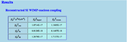
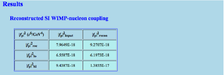
Figure 2: The reconstructed squared SI WIMP–nucleon coupling $|f_{\rm p}|^{2}$ by means of the method introduced in Ref. [3] with a ${}^{76}{\rm Ge}$ target. The commonly used value of the local Dark Matter density $\rho_{0}=0.3~{}{\rm GeV/cm^{3}}$ and a larger value of $\rho_{0}=0.4~{}{\rm GeV/cm^{3}}$ as well as the elastic nuclear form factors given in Eqs. (1) and (2) have been used for estimating $|f_{\rm p}|^{2}$ in the left and right frames, respectively.

Following the WIMP mass determination, I consider now the reconstruction of the SI WIMP coupling on nucleons $|f_{\rm p}|^{2}$ with a ${}^{76}{\rm Ge}$ target [3] .

In Figs. 2 I show the reconstructed squared SI WIMP-nucleon couplings and the lower and upper bounds of their 1$\sigma$ statistical uncertainties estimated by Eqs. (17) and (18) of Ref. [3] with an assumed (100$\pm$10 GeV, labeled with the subscript “input”) and the reconstructed (from Sec. 2.1, labeled with “recon”) WIMP masses. The commonly used value of the local Dark Matter density $\rho_{0}=0.3~{}{\rm GeV/cm^{3}}$ and a larger value of $\rho_{0}=0.4~{}{\rm GeV/cm^{3}}$ [15, 16, 17] as well as the elastic nuclear form factors given in Eqs. (1) and (2) have been used for estimating $|f_{\rm p}|^{2}$ in the left and right frames, respectively.

Among these results, the mean value and the overlap of two most plausible results (estimated with the reconstructed WIMP mass) give a rough 1$\sigma$ range of

$$|f_{\rm p}|^{2}\simeq 1.05_{-0.24}^{+0.33}\times 10^{-17}~{}{\rm GeV}^{-4}~{}\!,$$ (8)

or, equivalently,

$$|f_{\rm p}|\simeq 3.24_{-0.37}^{+0.51}\times 10^{-9}~{}{\rm GeV}^{-2}~{}\!.$$ (9)

Since the reconstructed WIMP mass given in Sec. 2.1 is $m_{\chi}\sim 115$ GeV, one can simply use the proton mass $m_{\rm p}$ to approximate the WIMP–proton reduced mass $m_{\rm r,p}$ and give a reconstructed SI WIMP–nucleon cross section as [10]

$$\sigma_{\chi{\rm p}}^{\rm SI}=\left(\frac{4}{\pi}\right)m_{\rm r,p}^{2}|f_{\rm p}|^{2}\approx\left(\frac{4}{\pi}\right)m_{\rm p}^{2}~{}\!|f_{\rm p}|^{2}\simeq 5.03_{-1.15}^{+1.58}\times 10^{-9}~{}{\rm pb}~{}\!.$$ (10)

2.3 Ratio of two spin–dependent WIMP–nucleon couplings $a_{\rm n}/a_{\rm p}$

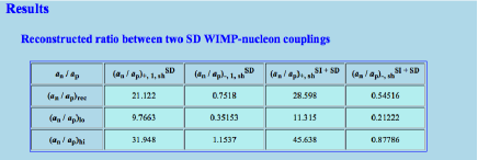
Figure 3: The reconstructed ratio between two SD WIMP–nucleon couplings, $a_{\rm n}/a_{\rm p}$, by means of two methods introduced in Ref. [4]. As usual, the elastic nuclear form factors given in Eqs. (1) and (2) have been used for determining $a_{\rm n}/a_{\rm p}$ in the left and right frames, respectively.

In Figs. 3 I show the reconstructed $a_{\rm n}/a_{\rm p}$ ratios and the lower and upper bounds of their 1$\sigma$ statistical uncertainties estimated by Eqs. (2.7) and (2.12) of Ref. [4] with $n=1$ as well as by Eqs. (3.16) and (3.20) of Ref. [4] at the shifted energy points [1, 4]. A combination of ${}^{19}{\rm F}$ + ${}^{127}{\rm I}$ targets has been used for the reconstruction of $a_{\rm n}/a_{\rm p}$ under the assumption that the SD WIMP–nucleus interaction dominates over the SI one (labeled with the superscript “SD”), whereas a third target of ${}^{28}{\rm Si}$ has been combined with ${}^{19}{\rm F}$ and ${}^{127}{\rm I}$ for the case of the general combination of both SI and SD WIMP interactions (labeled with the superscript “SI + SD”).

It can be found that, firstly, the “$+$ (plus)” solutions of the $a_{\rm n}/a_{\rm p}$ ratios given here are obviously too large to be the reasonable choice for $a_{\rm n}/a_{\rm p}$ and the “$-$ (minus)” solutions should be the correct ones. Secondly, although the reconstructed results under the assumption of the SD dominant WIMP interaction (third columns) is in general larger than the (in principle more plausible) results obtained without such a prior assumption (last columns), one could still use the mean value and the overlap of these two results to give a rough 1$\sigma$ range of

$$\frac{a_{\rm n}}{a_{\rm p}}\simeq 0.65_{-0.30}^{+0.23}~{}\!.$$ (11)

2.4 Ratios of the SD and SI WIMP–nucleon couplings $\sigma_{\chi({\rm p,n})}^{\rm SD}/\sigma_{\chi{\rm p}}^{\rm SI}$

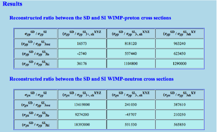
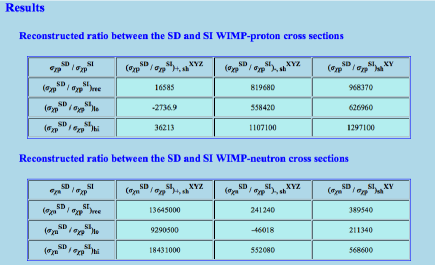
Figure 4: The reconstructed ratios between the SD and SI WIMP–nucleon couplings, $\sigma_{\chi({\rm p,n})}^{\rm SD}/\sigma_{\chi{\rm p}}^{\rm SI}$, by means of two methods introduced in Ref. [4]. As usual, the elastic nuclear form factors given in Eqs. (1) and (2) have been used for determining $\sigma_{\chi({\rm p,n})}^{\rm SD}/\sigma_{\chi{\rm p}}^{\rm SI}$ in the left and right frames, respectively.

In Figs. 4 I show the reconstructed $\sigma_{\chi({\rm p,n})}^{\rm SD}/\sigma_{\chi{\rm p}}^{\rm SI}$ ratios and the lower and upper bounds of their 1$\sigma$ statistical uncertainties estimated by Eqs. (3.9), (3.10) and (3.21) of Ref. [4] (with $a_{\rm n}/a_{\rm p}$ estimated by Eq. (3.16) of Ref. [4]) as well as by Eqs. (3.25) and (3.29) of Ref. [4] at the shifted energy points. A combination of data sets of ${}^{19}{\rm F}$, ${}^{127}{\rm I}$ and ${}^{28}{\rm Si}$ targets (labeled with the superscript “XYZ”) and that of data sets of ${}^{23}{\rm Na}$ or ${}^{131}{\rm Xe}$ with the (common) one of ${}^{76}{\rm Ge}$ (labeled with the superscript “XY”) have been used and the mean value and the overlap of these two results give a rough 1$\sigma$ range of

$$\frac{\sigma_{\chi{\rm p}}^{\rm SD}}{\sigma_{\chi{\rm p}}^{\rm SI}}\simeq 8.94_{-2.67}^{+2.13}\times 10^{5}~{}\!,~{}~{}~{}~{}~{}~{}~{}~{}~{}~{}~{}~{}~{}~{}~{}~{}\frac{\sigma_{\chi{\rm n}}^{\rm SD}}{\sigma_{\chi{\rm p}}^{\rm SI}}\simeq 3.16_{-1.05}^{+2.36}\times 10^{5}~{}\!.$$ (12)

Then, firstly, from these results one can further obtain that [10]

$$\left|\frac{a_{\rm n}}{a_{\rm p}}\right|\simeq 0.59_{-0.13}^{+0.23}~{}\!.$$ (13)

Secondly, combining the results in Eq. (12) with $\sigma_{\chi{\rm p}}^{\rm SI}$ given in Eq. (10), one can obtain that [10]

$$\sigma_{\chi{\rm p}}^{\rm SD}\simeq 4.50_{-1.69}^{+1.77}\times 10^{-3}~{}{\rm pb}~{}\!,~{}~{}~{}~{}~{}~{}~{}~{}~{}~{}~{}~{}~{}~{}~{}~{}\sigma_{\chi{\rm n}}^{\rm SD}\simeq 1.59_{-0.64}^{+1.08}\times 10^{-3}~{}{\rm pb}~{}\!.$$ (14)

These results give in turn that [10]

$$|a_{\rm p}|=0.112_{-0.021}^{+0.022}~{}\!,~{}~{}~{}~{}~{}~{}~{}~{}~{}~{}~{}~{}~{}~{}~{}~{}|a_{\rm n}|=0.067_{-0.013}^{+0.023}~{}\!.$$ (15)

On the other hand, one can also use the reconstructed $a_{\rm n}/a_{\rm p}$ ratio given in Eq. (11) and one of the two results given in Eq. (14) to obtain that [10]

$$\sigma_{\chi{\rm p}}^{\rm SD}\simeq 3.76_{-3.81}^{+3.69}\times 10^{-3}~{}{\rm pb}~{}\!,~{}~{}~{}~{}~{}~{}~{}~{}~{}~{}~{}~{}~{}~{}~{}~{}\sigma_{\chi{\rm n}}^{\rm SD}\simeq 1.90_{-1.89}^{+1.54}\times 10^{-3}~{}{\rm pb}~{}\!.$$ (16)

These results can also give that

$$|a_{\rm p}|\simeq 0.103_{-0.052}^{+0.050}~{}\!,~{}~{}~{}~{}~{}~{}~{}~{}~{}~{}~{}~{}~{}~{}~{}~{}|a_{\rm n}|\simeq 0.073_{-0.036}^{+0.030}~{}\!.$$ (17)

It can be found that, not surprisingly, the statistical uncertainties on the reconstructed $\sigma_{\chi({\rm p,n})}^{\rm SD}$ given in Eq. (16) are $\sim$ 2 or 3 times larger than those given in Eq. (14): Since $\sigma_{\chi({\rm p,n})}^{\rm SD}/\sigma_{\chi{\rm p}}^{\rm SI}$ reconstructed with the F + I + Si combination involve already the reconstructed $a_{\rm n}/a_{\rm p}$ ratio given in Eq. (11), the uncertainties on $\sigma_{\chi({\rm p,n})}^{\rm SD}$ given in Eq. (16) are thus overestimated. Secondly, the reconstructed $a_{\rm n}/a_{\rm p}$ ratio given in Eqs. (11) and (13) and the reconstructed $\sigma_{\chi({\rm p,n})}^{\rm SD}$ given in Eqs. (14) and (16) seem to match to each other pretty well.

The analyses given here show that, firstly, once one can estimate the SI WIMP–nucleon coupling/cross section, $|f_{\rm p}|$ or $\sigma_{\chi{\rm p}}^{\rm SI}$, and (one of) the ratios between the SD and SI WIMP–nucleon cross sections, and/or the ratio between two SD WIMP–nucleon couplings, the other couplings/cross sections could in principle be estimated. Secondly, the WIMP couplings/cross sections estimated in different way would be self–cross–checks to each other and the (in)compatibility between the reconstructed results would also help us to check the usefulness of the analyzed data sets offered from different experiments with different detector materials [14].

3 Input setup for generating pseudodata

In Table 1 I give finally the input setup for generating the pseudodata sets used in the analyses demonstrated in the previous section. For comparison, the reconstructed results shown in the previous section are also summarized here.

For generating WIMP signals, we used the commonly used form for the nuclear form factor given in Eq. (2) with another often used analytic form for $R_{1}$:

$$R_{1}=\sqrt{R_{A}^{2}+{\textstyle\left(\frac{7}{3}\right)}\pi^{2}r_{0}^{2}-5s^{2}}$$ (18)

with $R_{A}\simeq\big{(}1.23~{}\!A^{1/3}-0.6\big{)}~{}{\rm fm}$, $r_{0}\simeq 0.52~{}{\rm fm}$, $s\simeq 0.9~{}{\rm fm}$. Moreover, the shifted Maxwellian velocity distribution:

$$f_{1,{\rm sh}}(v)=\frac{1}{\sqrt{\pi}}\left(\frac{v}{v_{\rm e}v_{0}}\right)\bigg{[}e^{-(v-v_{\rm e})^{2}/v_{0}^{2}}-e^{-(v+v_{\rm e})^{2}/v_{0}^{2}}\bigg{]}$$ (19)

with the Sun’s Galactic orbital velocity $v_{0}=230$ km/s has been used; $v_{\rm e}$ is the time–dependent Earth’s velocity in the Galactic frame:

$$v_{\rm e}(t)=v_{0}\left[1.05+0.07\cos\left(\frac{2\pi(t-t_{\rm p})}{1~{}{\rm yr}}\right)\right]~{}\!,$$ (20)

where the date on which the Earth’s velocity relative to the WIMP halo is maximal has been set as $t_{\rm p}=140$ d. In addition, different from our setup used in Ref. [10], the experimental running date has been set as $t_{\rm expt}=100$ d and thus $v_{\rm e}(t_{\rm expt})=254$ km/s, much larger than the usually used values: $200~{}{\rm km/s}\leq v_{\rm e}\leq 240~{}{\rm km/s}$. Although these values for the astronomical setup are non–standard, we would like to stress that, as shown in the previous section and Table I, such a non–standard halo (model) would not affect the reconstructed results, since for using the AMIDAS package and website to analyze (real) data sets, one needs only the form factors for SI and/or SD WIMP–nucleaus cross sections, prior knowledge/assumptions about the WIMP velocity distribution $f_{1}(v)$ and local density $\rho_{0}$ (except the estimation of the SI WIMP–nucleon coupling $|f_{\rm p}|^{2}$) are not required.

Property	Reconstructed value	Input/Estimated value	Remarks
$m_{\chi}$	$115_{-35}^{+75}$ GeV	130 GeV
$\sigma_{\chi{\rm p}}^{\rm SI}$	$5.03_{-1.15}^{+1.58}\times 10^{-9}$ pb	$4\times 10^{-9}$ pb	$f_{\rm n}=f_{\rm p}$
$|f_{\rm p}|^{2}$	$1.05_{-0.24}^{+0.33}\times 10^{-17}~{}{\rm GeV}^{-4}$	$9.305\times 10^{-18}~{}{\rm GeV^{-4}}$	$\dagger$
$|f_{\rm p}|$	$3.24_{-0.37}^{+0.51}\times 10^{-9}~{}{\rm GeV}^{-2}$	$3.050\times 10^{-9}~{}{\rm GeV}^{-2}$	$\dagger$
$a_{\rm p}$	$0.112_{-0.021}^{+0.022}$	0.1
$a_{\rm n}$	$0.067_{-0.013}^{+0.023}$	0.07
$a_{\rm n}/a_{\rm p}$	$0.65_{-0.30}^{+0.23}$, $0.59_{-0.13}^{+0.23}$	0.7
$\sigma_{\chi{\rm p}}^{\rm SD}$	$4.50_{-1.69}^{+1.77}\times 10^{-3}$ pb	$3.51\times 10^{-3}$ pb	$\dagger$
$\sigma_{\chi{\rm n}}^{\rm SD}$	$1.59_{-0.64}^{+1.08}\times 10^{-3}$ pb	$1.72\times 10^{-3}$ pb	$\dagger$
$\sigma_{\chi{\rm p}}^{\rm SD}/\sigma_{\chi{\rm p}}^{\rm SI}$	$8.94_{-2.67}^{+2.13}\times 10^{5}$	$8.77\times 10^{5}$	$\dagger$
$\sigma_{\chi{\rm n}}^{\rm SD}/\sigma_{\chi{\rm p}}^{\rm SI}$	$3.16_{-1.05}^{+2.36}\times 10^{5}$	$4.30\times 10^{5}$	$\dagger$
$F_{\rm SI}^{2}(Q)$		$F_{\rm SI}^{2}(Q)$ in Eq. (2)	$\ddagger$
$F_{\rm SD}^{2}(Q)$		$F_{\rm TS}^{2}(Q)$ in Eq. (6)
$\rho_{0}$		$0.4~{}{\rm GeV/cm^{3}}$
$t_{\rm p}$		140 d
$t_{\rm expt}$		100 d	$\ddagger$
$v_{0}$		$230~{}{\rm km/s}$
$v_{\rm max}$		$600~{}{\rm km/s}$
$v_{\rm e}(t_{\rm expt})$		$253.9~{}{\rm km/s}$	$\ddagger$
$r_{\rm bg}$		0.12	$\ddagger$

Table 1: The input setup for generating the pseudodata sets used in the analyses demonstrated in this article. The theoretically estimated values and the reconstructed results are also given. $\dagger$: estimated for 130 GeV $m_{\chi}$; $\ddagger$: different from Ref. [10].

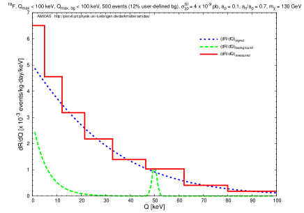
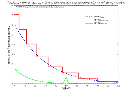
Figure 5: Measured energy spectra (solid red histograms) for a ${}^{19}{\rm F}$ (left) and a ${}^{76}{\rm Ge}$ (right) targets. The dotted blue curves are the elastic WIMP–nucleus scattering spectra, whereas the dashed green curves are the exponential background spectra combined with the Gaussian excesses ($r_{{\rm Gau}}=1$, $Q_{\rm bg,peak}=50$ keV and $\sigma_{Q,{\rm bg}}=1$ keV) and normalized to fit to the chosen background ratio $r_{\rm bg}=12\%$. See the text for further details.

On the other hand, for generating background events, the target–dependent exponential form for the residue background spectrum introduced in Ref. [11]:

$$\left(\frac{dR}{dQ}\right)_{\rm bg,ex}=\exp\left(-\frac{Q/{\rm keV}}{A^{0.6}}\right)$$ (21)

has been used. Here $A$ is the atomic mass number of the target nucleus; the power index of $A$, 0.6, is an empirical constant, which has been chosen so that the exponential background spectrum is somehow similar to, but still different from the expected recoil spectrum of the target nuclei (see Figs. 5). Meanwhile, considering possible radioactivity with a characteristic energy, we combined the exponential background spectrum in Eq. (21) with a Gaussian excess:

$$\left(\frac{dR}{dQ}\right)_{\rm bg,Gau}=\frac{r_{{\rm Gau}}}{\sqrt{2\pi}\left(\sigma_{Q,{\rm bg}}/{\rm keV}\right)}\exp\left[-\frac{\left(Q-Q_{\rm bg,peak}\right)^{2}}{2\sigma_{Q,{\rm bg}}^{2}}\right]~{}\!,$$ (22)

where $Q_{\rm bg,peak}$ and $\sigma_{Q,{\rm bg}}$ are the characteristic energy and energy dispersion of this background excess, respectively; $r_{{\rm Gau}}$ is the ratio of this Gaussian excess to the exponential spectrum.

In Figs. 5 I show the measured energy spectra (solid red histograms) for a ${}^{19}{\rm F}$ (left) and a ${}^{76}{\rm Ge}$ (right) targets. The dotted blue curves are the elastic WIMP–nucleus scattering spectra, whereas the dashed green curves are the exponential background spectra given in Eq. (21) combined with the Gaussian excesses given in Eq. (22) ($r_{{\rm Gau}}=1$, $Q_{\rm bg,peak}=50$ keV and $\sigma_{Q,{\rm bg}}=1$ keV for both targets), which have been normalized so that the ratios of the areas under the background spectra to those under the (dotted blue) WIMP scattering spectra are equal to the background–signal ratio ($r_{\rm bg}=12\%$) in the whole data sets. The experimental threshold energies have been assumed to be negligible and the maximal cut–off energies are set as 100 keV. 500 total events on average in one experiment have been simulated.

It can be seen here that, firstly, due to the contribution of the unrejected background events in low energy ranges ($Q~{}\>\raisebox{-3.01385pt}{$\stackrel{{\scriptstyle\textstyle<}}{{\sim}}$}\>~{}20$ keV for ${}^{19}{\rm F}$ and $Q~{}\>\raisebox{-3.01385pt}{$\stackrel{{\scriptstyle\textstyle<}}{{\sim}}$}\>~{}40$ keV for ${}^{76}{\rm Ge}$), the counting rates at the first energy bins (one of the two important quantities required in our model–independent data analyses) have been (strongly) overestimated. Secondly, the Gaussian background excesses around $Q=50$ keV cause clearly overestimates of the event rates, which would not only contribute (significantly) to the estimates of $I_{n}=\sum_{\rm all~{}events}Q_{i}^{(n-1)/2}/F^{2}(Q_{i})$ [1], but also cause a larger statistical fluctuation [2].

Nevertheless, our results obtained by analyzing pseudodata sets of $\cal O$(50) total events showed that, firstly, the WIMP mass given in Eq. (7) can match the input value very well: the deviations between the input and the reconstructed values with different assumed nuclear form factors are  $\stackrel{{\scriptstyle\textstyle<}}{{\sim}}$  20% ( $\stackrel{{\scriptstyle\textstyle<}}{{\sim}}$  30 GeV). As discussed earlier, this indicates that, for the first approximation of giving/constraining the most plausible range of the WIMP mass with pretty few total events, the uncertainty on the nuclear form factor could be safely neglected.

Secondly, all WIMP–nucleon couplings/cross sections as well as the ratios between them have also been reconstructed with $\sim$ 2% to  $\stackrel{{\scriptstyle\textstyle<}}{{\sim}}$  30% deviations from the input/theoretically estimated values. Although the SI WIMP coupling $|f_{\rm p}|$ estimated with the larger (input) local Dark Matter density (right frame of Figs. 2) could be underestimated [3], one can at least give an upper bound on $|f_{\rm p}|$. Moreover, by combining different methods for estimating different (ratios between the) WIMP couplings/cross sections, one could in principle observe/confirm the (in)compatibility between these results and probably correct the reconstructed values.

4 Summary

In this article I demonstrated the data analysis results of extracted WIMP properties by using theoretically generated pseudodata for different target nuclei, taking into account some unrejected background events mixed in the analyzed data sets. As an extension as well as the complementarity of our earlier theoretical works, I combined reconstructed results of the (ratios between different) WIMP couplings/cross sections on nucleons to estimate each individual coupling/cross section. Hopefully, the AMIDAS package and website as well as this demonstration can help our experimental colleagues to analyze their real direct detection data in the near future and to determine (at least rough ranges of) properties of halo Dark Matter particles.

Acknowledgments

The author appreciates the ILIAS Project and the Physikalisches Institut der Universität Tübingen for kindly providing the opportunity of the collaboration and the technical support of the AMIDAS website. The author would also like to thank the friendly hospitality of the Kavli Institute for Theoretical Physics China at the Chinese Academy of Sciences (KITPC) during the DSU workshop and the “Dark Matter and New Physics” program. This work was partially supported by the National Science Council of R.O.C. under contract no. NSC-99-2811-M-006-031 as well as by the National Center of Theoretical Sciences, R.O.C..

References

References

- [1] Drees M and Shan C-L 2007 Reconstructing the velocity distribution of WIMPs from direct dark matter detection data J. Cosmol. Astropart. Phys. JCAP06(2007)011 (Preprint astro-ph/0703651)
- [2] Drees M and Shan C-L 2008 Model–independent determination of the WIMP mass from direct dark matter detection data J. Cosmol. Astropart. Phys. JCAP06(2008)012 (Preprint 0803.4477)
- [3] Shan C-L 2011 Estimating the spin–independent WIMP–nucleon coupling from direct dark matter detection data (Preprint 1103.0481)
- [4] Shan C-L 2011 Determining ratios of WIMP–nucleon cross sections from direct dark matter detection data J. Cosmol. Astropart. Phys. JCAP07(2011)005 (Preprint 1103.0482)
- [5] http://pisrv0.pit.physik.uni-tuebingen.de/darkmatter/index1.html
- [6] http://www-ilias.cea.fr/
- [7] http://pisrv0.pit.physik.uni-tuebingen.de/darkmatter/amidas/
- [8] Shan C-L 2010 The AMIDAS website: an online tool for direct dark matter detection experiments AIP Conf. Proc. 1200 1031 (Preprint 0909.1459)
- [9] Shan C-L 2009 Uploading user–defined functions onto the AMIDAS website (Preprint 0910.1971)
- [10] Shan C-L 2011 Analyzing direct dark matter detection data on the AMIDAS website (Preprint 1109.0125)
- [11] Chou Y-T and Shan C-L 2010 Effects of residue background events in direct dark matter detection experiments on the determination of the WIMP mass J. Cosmol. Astropart. Phys. JCAP08(2010)014 (Preprint 1003.5277)
- [12] Shan C-L 2010 Effects of residue background events in direct dark matter detection experiments on the reconstruction of the velocity distribution function of halo WIMPs J. Cosmol. Astropart. Phys. JCAP06(2010)029 (Preprint 1003.5283)
- [13] Shan C-L 2011 Effects of residue background events in direct dark matter detection experiments on the estimation of the spin–independent WIMP–nucleon coupling (Preprint 1103.4049)
- [14] Shan C-L 2011 Effects of residue background events in direct dark matter detection experiments on the determinations of ratios of WIMP–nucleon cross sections (Preprint 1104.5305)
- [15] Catena R and Ullio P 2010 A novel determination of the local dark matter density J. Cosmol. Astropart. Phys. JCAP08(2010)004 (Preprint 0907.0018)
- [16] Salucci P, Nesti F, Gentile G and Martins C F 2010 The dark matter density at the sun’s location Astron. Astrophys. 523 A83 (Preprint 1003.3101)
- [17] Pato M, Agertz O, Bertone G, Moore B and Teyssier R 2010 Systematic uncertainties in the determination of the local dark matter density Phys. Rev. D 82 023531 (Preprint 1006.1322)