Introduction of the generalized Lorenz gauge condition into the vector tensor theory

Abstract

We introduce the generalized Lorentz gauge condition in the theory of quantum electrodynamics into the general vector-tensor theories of gravity. Then we explore the cosmic evolution and the static, spherically symmetric solution of the four dimensional vector field with the generalized Lorenz gauge. We find that, if the vector field is minimally coupled to the gravitation, it behaves as the cosmological constant. On the other hand, if it is nonminimally coupled to the gravitation, the vector field could behave as vast matters in the background of the spatially flat Friedmann-Robertson-Walker Universe. But it may not be the case. The weak, strong and dominant energy conditions, the stability analysis of classical and quantum aspects would put constraints on the parameters and so the equation of state of matters would be greatly constrained.

I Introduction

The vector-tensor theories of gravity are first proposed by Will, Nordtvedt and Hellings will:72 . Then they are used in cosmology to model inflaton ford:89 , dark matter bek:04 and dark energy bel:08 . However, it is recently found that the Lorentz invariant vector-tensor theories are usually plagued by instabilities bel:09 picon:09 . On the contrary, the Lorentz violation vector field models kos:89 are special such that some of these models are free of instabilities el:06 . The well-known Einstein-aether theory ted:00 belongs to these special models. The remarkable difference of the Einstein-aether theory from the usual vector-tensor theory comes from the fact that the vector field is constrained to have constant norm. This constraint eliminates a wrong-sign kinetic term for the length-stretching mode ell:05 , hence giving the theory a chance to be viable.

The fixed-norm constraint in the Einstein-aether is achieved by the presence of a Lagrange multiplier field in the Lagrangian density. The Lagrange multiplier method presents the constraints on the motion of some physical quantities in nature. So taking into account some physical constraints on the motion of physical quantities, one can always introduce the Lagrange multiplier into the corresponding Lagrange function. Actually, using this method, Mukhanov, Brandenberger and Sornborger have early proposed a nonsingular universe by limiting the spacetime curvature to some finite values muk:92 .

Except for the fixed-norm constraint, are there any other constraints on the four-vector (four dimensional vector) field? The answer is yes. We remember that there is a unified formulation of quantum electrodynamics which has the Lagrangian as follows lau:67

$$\mathscr{L} = -\frac{1}{4}F_{\mu\nu}F^{\mu\nu}+\lambda\left(\nabla_{\mu}A^{\mu}-\frac{1}{2}\gamma\lambda\right)$$ (1)

$$-j_{\mu}A^{\mu}+\bar{\psi}\left(i\gamma_{\mu}\partial^{\mu}-m\right)\psi\;.$$

Here $j_{\mu}=e\bar{\psi}\partial_{\mu}\psi$ and $F_{\mu\nu}$ is the field strength tensor of Maxwell field. $\lambda$ is the Lagrange multiplier field which has the dimension of inverse length, $l^{-1}$. $\gamma$ is a dimensionless constant. The $\lambda$ term is the generalized Lorentz gauge. $\gamma=0,\ 1,\ 3$ correspond to the Landau gauge lan:56 , the Feynman gauge fey:49 and the Yennie-Fried gauge fri:58 , respectively. We see the generalized Lorentz gauge condition could also be understood as a constraint on the divergence of four-vector field $A^{\mu}$. Motivated by this point, we introduce the generalized Lorentz gauge condition into the general vector-tensor theories.

The paper is organized as follows. In section II, we explore the cosmic evolution and the static, spherically symmetric solution of the four-vector field which is minimally coupled to the gravitation. We find the field behaves as a cosmological constant. In section III, we investigate the cosmic evolution of the four-vector which is nonminimally coupled to the gravitation and find it could play the role of vast matters for some appropriate parameters. Section IV gives the conclusion and discussion.

We shall use the system of units in which $16\pi G=c=\hbar=4\pi\varepsilon_{0}=1$ and the metric signature $(-,\ +,\ +,\ +)$ throughout the paper.

II Cosmological Constant from the four-vector field with the Generalized Lorenz Gauge

II.1 cosmology

The most general form for the Lagrangian density with two derivatives acting on the four-vector field $A^{\mu}$ can be written as

$$\mathscr{L} = -c_{1}\nabla_{\mu}A^{\nu}\nabla^{\mu}A_{\nu}-c_{2}\left(\nabla_{\mu}A^{\mu}\right)^{2}-c_{3}\nabla_{\mu}A^{\nu}\nabla_{\nu}A^{\mu}$$ (2)

$$+\lambda\left(\nabla_{\mu}A^{\mu}-\frac{1}{2}\gamma\lambda\right)\;.$$

Here $c_{i}$ are dimensionless constants. The stability analysis of the theory and the phenomenological investigations could put constraints on the sign and value of $c_{i}$.

Following the Einstein-aether theory carroll:2004 , If we define

$$J^{\mu}_{\ \ \nu} \equiv -c_{1}\nabla^{\mu}A_{\nu}-c_{2}\delta^{\mu}_{\nu}\nabla_{\alpha}A^{\alpha}-c_{3}\nabla_{\nu}A^{\mu}\;,$$

$$K^{\mu}_{\ \ \nu} \equiv \lambda\delta^{\mu}_{\nu}\;,$$ (3)

we can rewrite the Lagrangian density as follows

$$\mathscr{L} = J^{\mu}_{\ \ \nu}\nabla_{\mu}A^{\nu}+K^{\mu}_{\ \ \nu}\nabla_{\mu}A^{\nu}-\frac{1}{2}\gamma\lambda^{2}\;.$$ (4)

Variation of the Lagrangian density with respect to $A^{\mu}$ leads to the equation of motion for $A^{\mu}$

$$\nabla_{\mu}J^{\mu}_{\ \ \nu}+\nabla_{\mu}K^{\mu}_{\ \ \nu}+\frac{1}{2}\nabla_{\nu}\lambda=0\;.$$ (5)

On the other hand, variation of the Lagrangian density with respect to $\lambda$ gives the generalized Lorenz gauge condition

$$\nabla_{\mu}A^{\mu}-\gamma\lambda=0\;,$$ (6)

from which we can derive the Lagrange multiplier field $\lambda$. Acting on both sides of Eq. (6) by $\nabla_{\nu}$ and using Eq. (5), we find

$$\gamma\nabla_{\mu}J^{\mu}_{\ \ \nu}+\gamma\nabla_{\mu}K^{\mu}_{\ \ \nu}+\frac{1}{2}\nabla_{\nu}\left(\nabla_{\mu}A^{\mu}\right)=0\;.$$ (7)

This equation determines the dynamics of $A^{\mu}$ subject to the generalized Lorenz gauge condition.

The energy-momentum tensor for the vector field is found to be

$$T_{\mu\nu} = 2c_{1}\left(\nabla_{\alpha}A_{\mu}\nabla^{\alpha}A_{\nu}-\nabla_{\mu}A_{\alpha}\nabla^{\mu}A_{\alpha}\right)$$ (8)

$$+2\nabla_{\sigma}\left[J^{\ \ \sigma}_{(\mu}A_{\nu)}-J^{\sigma}_{\ \ (\mu}A_{\nu)}-J_{(\mu\nu)}A^{\sigma}\right]$$

$$+\nabla_{\sigma}\left[K^{\ \ \sigma}_{(\mu}A_{\nu)}-K^{\sigma}_{\ \ (\mu}A_{\nu)}-K_{(\mu\nu)}A^{\sigma}\right]$$

$$+g_{\mu\nu}\mathscr{L}\;.$$

In the background of spatially flat Friedmann-Robertson-Walker (FRW) Universe, the nonvanishing component of the vector is the timelike component. So the vector field $A^{\mu}$ can be written as

$$A^{\mu}=\left[\phi\left(t\right),\ 0,\ 0,\ 0\right]\;.$$ (9)

Then the equation of motion, Eq. (7), becomes

$$-\left(c_{1}+c_{2}+c_{3}-\frac{1}{2\gamma}\right)\left(\ddot{\phi}+3H\dot{\phi}+3\dot{H}\phi\right)$$

$$-3H^{2}\phi\left(c_{1}+c_{3}\right)=0\;,$$ (10)

where

$$H=\frac{\dot{a}}{a}\;,$$ (11)

is the Hubble parameter. $a(t)$ is the scale factor of the Universe. Dot denotes the derivative with respect to the cosmic time $t$. If

$$c_{1}+c_{3}=0\;,$$ (12)

the equation of motion, Eq. (II.1), reduces to a very simple case

$$\ddot{\phi}+3H\dot{\phi}+3\dot{H}\phi=0\;.$$ (13)

Solving the equation, we obtain

$$\dot{\phi}+3H{\phi}=\Lambda\;,$$ (14)

where $\Lambda$ is an integration constant which has the dimension of $l^{-1}$. Thus under the condition that Eq. (12) is satisfied, the Lagrangian, Eq. (2) turns out to be

$$\mathscr{L} = -\frac{c_{1}}{2}F_{\mu\nu}F^{\mu\nu}-c_{2}\left(\nabla_{\mu}A^{\mu}\right)^{2}$$ (15)

$$+\lambda\left(\nabla_{\mu}A^{\mu}-\frac{1}{2}\gamma\lambda\right)\;,$$

where

$$F_{\mu\nu} = \nabla_{\mu}A_{\nu}-\nabla_{\nu}A_{\mu}\;,$$ (16)

is the field strength tensor.

In this paper, we are interested in the case of $c_{1}+c_{3}=0$ for simplicity. From the generalized Lorenz gauge condition, Eq. (6), we obtain

$$\dot{\phi}+3H{\phi}=\gamma\lambda\;.$$ (17)

Taking account of Eq. (14), we find the Lagrange multiplier field is actually a constant,

$$\lambda=\frac{\Lambda}{\gamma}\;.$$ (18)

So we can solve for $\phi$ from Eq. (17) as follows

$$\phi=\frac{\Lambda}{a^{3}}\int a^{3}dt\;.$$ (19)

Then the energy density and pressure of the vector field derived from the energy-momentum tensor take the form

$$\rho_{A} = -T_{0}^{0}=\left(-c_{2}+\frac{1}{2\gamma}\right)\Lambda^{2}\;,$$

$$p_{A} = T_{i}^{i}=-\left(-c_{2}+\frac{1}{2\gamma}\right)\Lambda^{2}\;.$$ (20)

This is exactly for the energy density and pressure of Einstein’s cosmological constant. To interpret the current acceleration of the Universe, we expect $\Lambda$ to be the order of the inverse of present-day Hubble length and

$$-c_{2}+\frac{1}{2\gamma}>0\;.$$ (21)

If $c_{2}=0$, we conclude that $\gamma$ must be positive. The Feynman and Yennie-Fried gauge satisfy this requirement, while the Landau gauge leads to a vanishing cosmological constant.

II.2 static and spherically symmetric solution

In order to show the four-vector field theory can pass the solar system tests, in this subsection, let’s seek for the static and spherically symmetric solution of Einstein equations sourced by the Lagrangian Eq. (15). The static and spherically symmetric metric can always be written as

$$ds^{2}=-U\left(r\right)dt^{2}+\frac{1}{U\left(r\right)}dr^{2}+f\left(r\right)^{2}d\Omega^{2}\;.$$ (22)

Comparing to solving the Einstein equations, we prefer to start from the Lagrangian Eq. (15) for simplicity in calculations. Because of the static and spherically symmetric property of the spacetime, the vector field $A_{\mu}$ takes the form

$$A_{\mu}=\left[\phi\left(r\right),\ \psi\left(r\right),\ 0,\ 0\right]\;,$$ (23)

where $\phi$ and $\psi$ correspond to the electric and magnetic part of the electromagnetic potential. Then we have

$$F_{\mu\nu}F^{\mu\nu}=-2\phi^{{}^{\prime}2}\;,\ \ \ \nabla_{\mu}A^{\mu}=\left(U\psi\right)^{{}^{\prime}}+2\frac{f^{{}^{\prime}}}{f}U\psi\;,$$ (24)

where prime denotes the derivative with respect to $r$. Taking into account the Ricci scalar, $R$, we have the total Lagrangian from Eq. (15)

$$\mathscr{L} = -U^{{}^{\prime\prime}}-4U^{{}^{\prime}}\frac{f^{{}^{\prime}}}{f}-4U\frac{f^{{}^{\prime\prime}}}{f}+\frac{2}{f^{2}}-2U\frac{f^{{}^{\prime}2}}{f^{2}}$$ (25)

$$+{c_{1}}\phi^{{}^{\prime}2}-c_{2}\left[\left(U\psi\right)^{{}^{\prime}}+2\frac{f^{{}^{\prime}}}{f}U\psi\right]^{2}$$

$$+\lambda\left[\left(U\psi\right)^{{}^{\prime}}+2\frac{f^{{}^{\prime}}}{f}U\psi-\frac{1}{2}\gamma\lambda\right]\;.$$

Using the Euler-Lagrange equation, we obtain the equation of motion for $\phi$,

$$f\phi^{{}^{\prime\prime}}+2\phi^{{}^{\prime}}f^{{}^{\prime}}=0\;,$$ (26)

for $\lambda$,

$$\left(U\psi\right)^{{}^{\prime}}+2\frac{f^{{}^{\prime}}}{f}U\psi-\gamma\lambda=0\;,$$ (27)

for $U$,

$$2ff^{{}^{\prime\prime}}-4c_{2}f\psi^{2}U^{{}^{\prime}}f^{{}^{\prime}}-4c_{2}\psi f^{2}U^{{}^{\prime}}\psi^{{}^{\prime}}-2c_{2}\psi^{2}f^{2}U^{{}^{\prime\prime}}$$

$$-4c_{2}\psi Uf\psi^{{}^{\prime}}f^{{}^{\prime}}+4c_{2}U\psi^{2}f^{{}^{\prime}2}-2c_{2}\psi Uf^{2}\psi^{{}^{\prime\prime}}$$

$$-4c_{2}Uf\psi^{2}f^{{}^{\prime\prime}}+\psi f^{2}\lambda^{{}^{\prime}}=0\;,$$ (28)

for $\psi$,

$$-4c_{2}U\psi ff^{{}^{\prime\prime}}-4c_{2}f\psi U^{{}^{\prime}}f^{{}^{\prime}}-4c_{2}f^{2}U^{{}^{\prime}}\psi^{{}^{\prime}}-2c_{2}\psi f^{2}U^{{}^{\prime\prime}}$$

$$-4c_{2}Uf\psi^{{}^{\prime}}f^{{}^{\prime}}+4c_{2}U\psi f^{{}^{\prime}2}-2c_{2}Uf^{2}\psi^{{}^{\prime\prime}}$$

$$+f^{2}\lambda^{{}^{\prime}}=0\;,$$ (29)

and for$f$,

$$-2c_{1}f\phi^{{}^{\prime}2}-4c_{2}Uf\psi^{2}U^{{}^{\prime\prime}}-12c_{2}U\psi fU^{{}^{\prime}}\psi^{{}^{\prime}}-4c_{2}U^{2}\psi f\psi^{{}^{\prime\prime}}$$ (30)

$$-16c_{2}U\psi^{2}U^{{}^{\prime}}f^{{}^{\prime}}-16c_{2}U^{2}\psi\psi^{{}^{\prime}}f^{{}^{\prime}}-8c_{2}U^{2}\psi^{2}f^{{}^{\prime\prime}}$$

$$-2c_{2}f\psi^{2}U^{{}^{\prime}2}+\gamma f\lambda^{2}+4U^{{}^{\prime}}f^{{}^{\prime}}+4Uf^{{}^{\prime\prime}}+2fU^{{}^{\prime\prime}}$$

$$+2Uf\psi\lambda^{{}^{\prime}}-2c_{2}fU^{2}\psi^{{}^{\prime}2}\;,$$

respectively. Now we have five independent differential equations and five unknown variables, $U,\ f,\ \phi,\ \psi,\ \lambda$. So the system of equations is closed.

From Eq. (26), we obtain

$$\phi=\phi_{1}+\phi_{0}\int\frac{1}{f^{2}}dr\;,$$ (31)

where $\phi_{0},\ \phi_{1}$ are two integration constants. In order to fix $\phi_{1}$, let us consider the asymptotic condition, namely, for large enough $r$. We expect to have $f^{2}\sim r^{2}$. So $\phi\sim\phi_{1}+\phi_{0}/r$. Let the asymptotic value of $\phi=0$ when $r$ is large enough. Then we conclude that

$$\phi_{1}=0\;.$$ (32)

On the other hand, from Eq. (27), we obtain

$$\lambda=\frac{1}{\gamma}\left[\left(U\psi\right)^{{}^{\prime}}+2\frac{f^{{}^{\prime}}}{f}U\psi\right]\;.$$ (33)

Keeping Eqs. (31), (32) and (33) in mind, we obtain from the difference of Eq.(II.2) and Eq. (II.2)

$$f^{{}^{\prime\prime}}=0\;.$$ (34)

So we have

$$f=f_{0}+f_{1}r\;.$$ (35)

$f_{0},\ f_{1}$ are two integration constants. We can always rescale $r$ such that

$$f_{0}=0\;,\ \ f_{1}=1\;.$$ (36)

Then we obtain from Eq. (II.2)

$$\psi=\frac{\psi_{0}r}{U}+\frac{\psi_{1}}{r^{2}U}\;,$$ (37)

with $\psi_{0},\ \psi_{1}$ two integration constants. Finally, Eq. (30) turns out to be

$$2\gamma r^{4}U^{{}^{\prime\prime}}+4\gamma r^{3}U^{{}^{\prime}}+9\psi_{0}^{2}r^{4}-2c_{1}\gamma\phi_{0}^{2}$$

$$-18c_{2}\gamma\psi_{0}^{2}r^{4}=0\;,$$ (38)

from which we obtain

$$U=U_{0}-\frac{U_{1}}{r}+\frac{c_{1}\phi_{0}^{2}}{2r^{2}}-\frac{3}{2}\left(-c_{2}+\frac{1}{2\gamma}\right)\psi_{0}^{2}r^{2}\;,$$ (39)

where $U_{0}$ and $U_{1}$ are two integration constants. Compare it with the Reissner-Nordstrom-de Sitter solution

$$U=1-\frac{2M}{r}+\frac{Q^{2}}{r^{2}}-\frac{1}{6}Lr^{2}\;,$$ (40)

we may put

$$U_{0}=1\;,\ \ \ U_{1}=2M\;,\ \ \ c_{1}=2\;,\ \ \phi_{0}=Q\;,\ \$$

$$\psi_{0}=\frac{\Lambda}{3}\;,\ \ \ L=\left(-c_{2}+\frac{1}{2\gamma}\right)\Lambda^{2}\;.$$ (41)

Here $L$ denotes the cosmological constant.

Therefore, the static and spherically solution for the Lagrangian density, Eq. (15), is exactly the Reissner-Nordstrom-de Sitter solution. The field $\phi,\ \psi$ and the Lagrange multiplier $\lambda$ is found to be

$$\phi=\frac{Q}{r}\;,\ \ \ \lambda=\frac{\Lambda}{\gamma}\;,\ \ \psi=\frac{\Lambda r}{3U}+\frac{\psi_{1}}{r^{2}U}\;.$$ (42)

We recognize that $\phi$ is the electric potential sourced by the change $Q$. The cosmological constant is closely related to the field strength $\partial_{r}(r^{2}U\psi)$ of the magnetic potential $\psi$. Since the static and spherically symmetric solution of the theory is just the Reissner-Nordstrom-de Sitter solution, we conclude that it would not violate the solar system tests on gravity theory.

III nonminimally coupled to gravitation

III.1 equations of motion and energy momentum tensor

When the four-vector $A^{\mu}$ is nonminimally coupled to the gravitation, we have the Lagrangian density as follows:

$$\mathscr{L} = -\frac{c_{1}}{2}F_{\mu\nu}F^{\mu\nu}-c_{2}\left(\nabla_{\mu}A^{\mu}\right)^{2}+b_{1}R_{\mu\nu}A^{\mu}A^{\nu}$$ (43)

$$+b_{2}RA_{\mu}A^{\nu}+\lambda\left(\nabla_{\mu}A^{\mu}-\frac{1}{2}\gamma\lambda\right)\;.$$

Here $b_{1},\ b_{2}$ are two dimensionless constants and $R_{\mu\nu},\ R$ are the Ricci tensor and the Ricci scalar, respectively. In the first place, varying the Lagrangian density with respect to $A^{\mu}$, we obtain the equation of motion for $A^{\mu}$

$$c_{1}\nabla_{\nu}F^{\nu}_{\ \ \mu}+c_{2}\nabla_{\mu}\left(\nabla_{\nu}A^{\nu}\right)+b_{1}R_{\mu\nu}A^{\nu}$$

$$+b_{2}RA_{\mu}-\frac{1}{2}\nabla_{\mu}\lambda=0\;.$$ (44)

Secondly, varying the Lagrangian density with respect to $\lambda$, we obtain the equation of motion for $\lambda$

$$\nabla_{\mu}A^{\mu}-\gamma\lambda=0\;.$$ (45)

Finally, varying the Lagrangian density with respect to $g^{\mu\nu}$, we obtain the energy momentum

$$T_{\mu\nu} = 2\nabla_{\sigma}\left[J^{\ \ \sigma}_{(\mu}A_{\nu)}-J^{\sigma}_{\ \ (\mu}A_{\nu)}-J_{(\mu\nu)}A^{\sigma}\right]$$ (46)

$$+\nabla_{\sigma}\left[K^{\ \ \sigma}_{(\mu}A_{\nu)}-K^{\sigma}_{\ \ (\mu}A_{\nu)}-K_{(\mu\nu)}A^{\sigma}\right]$$

$$+b_{1}\left[2\nabla_{\sigma}\nabla_{(\mu}\left(A_{\nu{)}}A^{\sigma}\right)-\nabla_{\alpha}\nabla_{\sigma}\left(A^{\alpha}A^{\sigma}\right)g_{\mu\nu}\right.$$

$$\left.-\nabla^{2}\left(A_{\mu}A_{\nu}\right)-4A^{\sigma}R_{\sigma(\mu}A_{\nu)}\right]-2b_{2}\left[R_{\mu\nu}A_{\sigma}A^{\sigma}\right.$$

$$\left.+RA_{\mu}A_{\nu}-\nabla_{\mu}\nabla_{\nu}\left(A_{\sigma}A^{\sigma}\right)+\nabla^{2}\left(A_{\sigma}A^{\sigma}\right)g_{\mu\nu}\right]$$

$$+2c_{1}F_{\mu\sigma}F^{\sigma}_{\ \ \nu}+g_{\mu\nu}\mathscr{L}\;.$$

Here $J_{\mu\nu}$ is understood with $c_{1}+c_{3}=0$. Combining Eq. (III.1) and Eq. (45), we can express the equation of motion for $A^{\mu}$ as follows

$$c_{1}\nabla_{\nu}F^{\nu}_{\ \ \mu}+c_{2}\nabla_{\mu}\left(\nabla_{\nu}A^{\nu}\right)+b_{1}R_{\mu\nu}A^{\nu}$$

$$+b_{2}RA_{\mu}-\frac{1}{2\gamma}\nabla_{\mu}\left(\nabla_{\nu}A^{\nu}\right)=0\;.$$ (47)

III.2 cosmic evolution

In the background of spatially flat FRW Universe, the equations of motion, Eq. (III.1) takes the form

$$\left(c_{2}-\frac{1}{2\gamma}\right)\left(\dot{\phi}+3H\phi\right)^{\cdot}-3\left(b_{1}+2b_{2}\right)\dot{H}\phi$$

$$-3H^{2}\phi\left(b_{1}+4b_{2}\right)=0\;.$$ (48)

From the energy momentum tensor, we obtain the energy density and pressure of the four-vector field $A^{\mu}$

$$\rho_{A} = c_{2}\left(2\phi\ddot{\phi}-\dot{\phi}^{2}\right)+6\left(b_{1}+2b_{2}\right)H\phi\dot{\phi}$$ (49)

$$+\left[6\left(c_{2}-b_{1}-2b_{2}\right)\dot{H}-9\left(c_{2}+2b_{2}\right)H^{2}\right]\phi^{2}$$

$$-\phi\dot{\lambda}+\frac{1}{2}\gamma\lambda^{2}\;,$$

$$p_{A} = 2\left(c_{2}-b_{1}-2b_{2}\right)\left(\phi\ddot{\phi}+\dot{\phi}^{2}\right)-c_{2}\dot{\phi}^{2}$$ (50)

$$+\left(3c_{2}-2b_{1}-2b_{2}\right)\left[4H\phi\dot{\phi}+\left(2\dot{H}+3H^{2}\right)\phi^{2}\right]$$

$$-\phi\dot{\lambda}+\frac{1}{2}\gamma\lambda^{2}\;.$$

Using the equation of motion for $A^{\mu}$, Eq. (III.2), and the generalized Lorentz gauge condition, Eq. (45), we can eliminate $\ddot{\phi}$ and rewrite the energy density as following

$$\rho_{A} = 6H\dot{\phi}\phi\left(-c_{2}+\frac{1}{2\gamma}+b_{1}+2b_{2}\right)$$ (51)

$$+9H^{2}\phi^{2}\left(-c_{2}+\frac{1}{2\gamma}+\frac{2}{3}b_{1}+\frac{2}{3}b_{2}\right)$$

$$+\left(-c_{2}+\frac{1}{2\gamma}\right)\dot{\phi}^{2}\;.$$

We have verified that the energy density, Eq. (51), and the pressure, Eq. (50), satisfy the energy conservation equation

$$\frac{d\rho_{A}}{dt}+3H\left(\rho_{A}+p_{A}\right)=0\;,$$ (52)

which is consistent with the equation of motion, Eq. (III.2) and the energy momentum conservation equation

$$\nabla_{\nu}T^{\nu}_{\ \ \mu}=0\;.$$ (53)

In other words, the equation of motion Eq. (III.2), the energy conservation equation Eq. (52) and the energy momentum conservation equation Eq. (53) give actually the same equation. Similarly, using the equation of motion for $A^{\mu}$, Eq. (III.2), and the generalized Lorentz gauge condition, Eq. (45), we can eliminate $\ddot{\phi}$ and rewrite the pressure as following

$$p_{A} = -\left(-c_{2}+\frac{1}{2\gamma}+2b_{1}+4b_{2}\right)\dot{\phi}^{2}$$ (54)

$$+\left(6c_{2}+4b_{2}-\frac{3}{\gamma}-2b_{1}\right)H\phi\dot{\phi}$$

$$-\frac{4\gamma}{2c_{2}\gamma-{1}}\left(\frac{2b_{1}}{\gamma}+\frac{5b_{2}}{\gamma}+12b_{2}^{2}+12b_{1}b_{2}\right.$$

$$\left.+3b_{1}^{2}-10c_{2}b_{2}-4c_{2}b_{1}\right)\dot{H}\phi^{2}$$

$$-\frac{3\gamma}{4c_{2}\gamma-2}H^{2}\phi^{2}\left(-\frac{3}{\gamma^{2}}+\frac{12b_{2}+12c_{2}}{\gamma}\right.$$

$$\left.+64b_{2}^{2}-12c_{2}^{2}+48b_{1}b_{2}+8b_{1}^{2}-24c_{2}b_{2}\right)\;.$$

Then we find

$$p_{A}-\frac{{1}-\left(2c_{2}-4b_{1}-8b_{2}\right)\gamma}{2c_{2}\gamma-1}\rho_{A}$$ (55)

$$= \frac{4}{1-2c_{2}\gamma}\phi\left(\phi\dot{H}+2H\dot{\phi}+3H^{2}\phi\right)$$

$$\cdot\left[\left(3b_{1}^{2}+12b_{2}^{2}-10c_{2}b_{2}+12b_{1}b_{2}-4c_{2}b_{1}\right)\gamma\right.$$

$$\left.+2b_{1}+5b_{2}\right]\;.$$

It is apparent if

$$b_{1}=b_{2}=0\;,$$ (56)

we have the equation of state for the four-vector $A^{\mu}$

$$\omega_{A}=\frac{p_{A}}{\rho_{A}}=-1\;,$$ (57)

which is consistent with the result of Eq. (II.1).

On the other hand, if $b_{1}\neq 0$ (or $b_{2}\neq 0$) and

$$\left(3b_{1}^{2}+12b_{2}^{2}-10c_{2}b_{2}+12b_{1}b_{2}-4c_{2}b_{1}\right)\gamma$$

$$+2b_{1}+5b_{2}=0\;,$$ (58)

namely,

$$\gamma=-\frac{2b_{1}+5b_{2}}{3b_{1}^{2}+12b_{2}^{2}-10c_{2}b_{2}+12b_{1}b_{2}-4c_{2}b_{1}}\;,$$ (59)

we have the equation of state

$$\omega_{A} = \frac{5b_{1}+14b_{2}}{3\left(b_{1}+2b_{2}\right)}$$ (60)

$$= \frac{14+5\frac{b_{1}}{b_{2}}}{3\left(2+\frac{b_{1}}{b_{2}}\right)}$$

$$= \frac{14+5r}{3\left(2+r\right)}\;,$$

where we define the ratio $r$ of $b_{1}$ and $b_{2}$ as $r=b_{1}/b_{2}$. In other words, if the value of $\gamma$ is given by Eq. (59), we shall have a constant equation of state for vector field $A^{\mu}$.

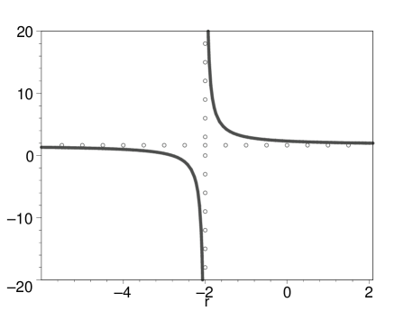
Figure 1: The equation of state $w_{A}$ of the four-vector field $A^{\mu}$ with the ratio $r$ of $b_{1}$ and $b_{2}$. It is not bounded both below and up, namely, $-\infty<w_{A}<+\infty$.

In Fig. 1, we plot the equation of state $\omega_{A}$ of the four-vector field $A^{\mu}$ with the ratio $r$ of $b_{1}$ and $b_{2}$. It is not bounded both below and up, namely, $-\infty<w<+\infty$. This is different from the quintessence which has the equation of state $-1\leq w\leq+1$.

In particular, when

$$b_{2}=-\frac{5}{14}b_{1}\;,\ \ \ \gamma=\frac{7}{2\left(7c_{2}-4b_{1}\right)}\;,$$ (61)

we have the equation of state

$$\omega_{A}=0\;,$$ (62)

which indicates that the four-vector field $A^{\mu}$ behaves as a dust matter. So the four-vector field could behave as vast matters in the background of spatially flat FRW Universe. However, this may be not the case. The weak, strong and dominant energy conditions wald:84 , the stability analysis of classical and quantum aspects would put constraints on the parameters and so the equation of state would be greatly constrained.

IV Conclusion and discussion

In conclusion, motivated by the Lagrange multiplier method in the Einstein-aether theory, we introduce the generalized Lorentz gauge condition in the theory of quantum electrodynamics into the general vector-tensor theories of gravity. With the fix-norm constraint, it is found that the Einstein-aether field contributes an energy density carroll:2004

$$\rho_{A}=-3\left(c_{1}+3c_{2}+c_{3}\right)m^{2}H^{2}\;,$$ (63)

where the constant $m$ represents the norm of the four-vector $A^{\mu}$. In order that the energy density be positive, one should have $c_{1}+3c_{2}+c_{3}<0$. However, as shown by Lim, the investigations of quantum aspect on this theory require $c_{1}+3c_{2}+c_{3}\geq 0$ lim:04 . Therefore, the energy density of the aether field is nonpositive which violets the weak energy condition wald:84 .

However, with the generalized Lorentz gauge condition, we find that the vector filed could contribute a constant energy density. For the minimally coupled case, in particular, when $c_{1}=-c_{3},\ c_{2}=0$, we always have a non-negative energy density for the Landau gauge, Feynman gauge and Yennie-Fried gauge. The corresponding quantum aspects have been very well studied. On the other hand, the static and spherically symmetric solution sourced by the vector field is exactly the Reissner-Nordstrom-de Sitter solution. This reveals that the theory may not be conflict with the solar system tests on gravity theory. For the non-minimally coupled case, the vector may play the role of vast matters in the background of spatially flat Universe. But it may be not the case. The stability analysis of classical and quantum aspects would surely constrain the space of parameters. It is a very important issue. We plan to leave this analysis for future publications.

References

• (1) C. M. Will and K. Nordtvedt Jr., Astrophys. J., 177, 757 (1972); K. Nordtvedt Jr. and C. M. Will, Astrophys. J., 177, 775 (1972); R. W. Hellings and K. Nordtvedt Jr., Phys. Rev. D7, 3593 (1973).
• (2) L. H. ford,  Phys. Rev. D 35, 2339 (1987); A. B. Burd and J. E. Lidsey, Nucl. Phys. B351, 679 (1991); A. Golovnev, V. Mukhanov and V. Vanchurin, JCAP 0806, 009 (2008); T. Koivisto and D. F. Mota, JCAP 0808, 021 (2008); S. Kanno and J. Soda,  Phys. Rev. D 74, 063505 (2006); M. A. Watanabe, S. Kanno and J. Soda, arXiv:0902.2833 [hep-th].
• (3) J. D. Bekenstein,  Phys. Rev. D 70, 083509 (2004); T. G. Zlosnik, P. G. Ferreira and G. D. Starkman,  Phys. Rev. D 75, 044017 (2007).
• (4) J. B. Jimenez, A. L. Maroto, JCAP.  0903, 016  (2009);  Phys. Rev. D 80, 063512 (2009); J. Beltran Jim enez and A.L. Maroto,  Phys. Rev. D 78, 063005 (2008); J. Beltran Jim enez and A.L. Maroto, e-Print: arXiv:0807.2528; J. Beltran Jim enez, Ruth Lazkoz and A.L. Maroto, e-Print: arXiv:0904.0433 [astro-ph.CO]; H. Wei and R. G. Cai,  Phys. Rev. D 73, 083002 (2006); H. Wei and R. G. Cai,  JCAP.  0709, 015  (2007); J. Beltr an Jim enez and A. L. Maroto, JCAP 0903: 016 (2009); J. Beltr an Jim enez and A. L. Maroto, e-Print: arXiv:0812.1970 [astro-ph]; J. Beltr an Jim enez and A. L. Maroto, e-Print: arXiv:0903.4672 [astro-ph.CO]; Christian Armendariz-Picon,  JCAP.  0407, 007  (2004); V. V. Kiselev,  Class. Quant. Grav. 21, 3323 (2004); M. Novello, Santiago Esteban Perez Bergliaffa, and J. Salim,  Phys. Rev. D 69, 127301 (2004); X. H. Meng and X. L. Du, astro-ph/1109.0823; C. Gao, Y. Gong, X. Wang and X. Chen,  Phys. Lett. B 702, 107 (2011).
• (5) J. Beltr an Jim enez and A. L. Maroto JCAP 0902: 025 (2009).
• (6) C. Armendariz-Picon and A. Diez-Tejedor,  JCAP.  0912, 018  (2009) astro-ph/0904.0809.
• (7) V. A. Kostelecky and S. Samuel, Phys. Rev. D 40 1886 (1989); C. Eling, T. Jacobson and D. Mattingly, gr-qc/0410001; R. Bluhm and V. A. Kostelecky, Phys. Rev. D71 065008 (2005); Q. G. Bailey and V. A. Kostelecky, Phys. Rev. D74 045001 (2006); R. Bluhm, S. H. Fung and V. A. Kostelecky, Phys. Rev. D77 065020 (2008); R. Bluhm, N. L. Gagne, R. Potting and A. Vrublevskis, Phys. Rev. D77 125007 (2008).
• (8) C. Eling, Phys. Rev. D73, 084026 (2006); S. M. Carroll, T. R. Dulaney, M. I. Gresham, H. T. Phys. Rev.D79: 065011 (2009); S. M. Carroll, T. R. Dulaney, M. I. Gresham, H. T. Phys. Rev.D79: 065012 (2009); Sean. M. Caroll, et al, Phys. Rev. D 79, 065011 (2009); C. Armendariz-Picon, N. F. Sierra and J. Garriga,  JCAP.  07, 010  (2010);
• (9) T. Jacobson and D. Mattingly,  Phys. Rev. D 64, 024028 (2001). [arXiv:grqc/ 0007031].
• (10) J. W. Elliott, G. D. Moore and H. Stoica,  JHEP. 0508, 066 (2005). [arXiv:hepph/ 0505211].
• (11) V. Mukhanov and R. Brandenberger,  Phys. Rev. Lett. 68, 1969 (1992); R. Brandenberger, V. Mukhanov and A. Sornborger,  Phys. Rev. D 48, 1629 (1993).
• (12) B. Lautrup, Kgl. Danske Videnskab. Selskab, Mat.-fys. Medd. 35, Vol. 11 (1967), sec. 8.2.
• (13) L. D. Landau and I. M. Khalatnikov, Sov. Phys. JETP 2, 69 (1956).
• (14) R. P. Feynman, Phys. Rev. 76, 769 (1949).
• (15) H. M. Fried and D. R. Yennie, Phys. Rev. 112, 1391 (1958).
• (16) S. M. Carroll and E. A. Lim,  Phys. Rev. D 70, 123525 (2004).
• (17) R. M. Wald, Genreral Relativity, (Chicago: University of Chicago Press) (1984).
• (18) E. A. Lim, (2004),  Phys. Rev. D 71, 063504 (2005).