Compressive Phase Retrieval From Squared Output Measurements Via Semidefinite Programming
Abstract
Given a linear system in a real or complex domain, linear regression aims to recover the model parameters from a set of observations. Recent studies in compressive sensing have successfully shown that under certain conditions, a linear program, namely, -minimization, guarantees recovery of sparse parameter signals even when the system is underdetermined. In this paper, we consider a more challenging problem: when the phase of the output measurements from a linear system is omitted. Using a lifting technique, we show that even though the phase information is missing, the sparse signal can be recovered exactly by solving a simple semidefinite program when the sampling rate is sufficiently high, albeit the exact solutions to both sparse signal recovery and phase retrieval are combinatorial. The results extend the type of applications that compressive sensing can be applied to those where only output magnitudes can be observed. We demonstrate the accuracy of the algorithms through theoretical analysis, extensive simulations and a practical experiment.
1 Introduction
Linear models, e.g. , are by far the most used and useful type of model. The main reasons for this are their simplicity of use and identification. For the identification, the least-squares (LS) estimate in a complex domain is computed by111Our derivation in this paper is primarily focused on complex signals, but the results should be easily extended to real domain signals.
| (1) |
assuming the output and are given. Further, the LS problem has a unique solution if the system is full rank and not underdetermined, i.e. .
Consider the alternative scenario when the system is underdetermined, i.e. . The least squares solution is no longer unique in this case, and additional knowledge has to be used to determine a unique model parameter. Ridge regression or Tikhonov regression [Hoerl and Kennard, 1970] is one of the traditional methods to apply in this case, which takes the form
| (2) |
where is a scalar parameter that decides the trade off between fit in the first term and the -norm of in the second term.
Thanks to the -norm regularization, ridge regression is known to pick up solutions with small energy that satisfy the linear model. In a more recent approach stemming from the LASSO [Tibsharani, 1996] and compressive sensing (CS) [Candès et al., 2006, Donoho, 2006], another convex regularization criterion has been widely used to seek the sparsest parameter vector, which takes the form
| (3) |
Depending on the choice of the weight parameter , the program (3) has been known as the LASSO by Tibsharani [1996], basis pursuit denoising (BPDN) by Chen et al. [1998], or -minimization (-min) by Candès et al. [2006]. In recent years, several pioneering works have contributed to efficiently solving sparsity minimization problems such as [Tropp, 2004, Beck and Teboulle, 2009, Bruckstein et al., 2009], especially when the system parameters and observations are in high-dimensional spaces.
In this paper, we consider a more challenging problem. In a linear model , rather than assuming that is given, we will assume that only the squared magnitude of the output is observed:
| (4) |
where , and denotes the Hermitian transpose of . This is clearly a more challenging problem since the phase of is lost when only its (squared) magnitude is available. A classical example is that represents the Fourier transform of , and that only the Fourier transform modulus is observable. This scenario arises naturally in several practical applications such as optics [Walther, 1963, Millane, 1990], coherent diffraction imaging [Fienup, 1987], and astronomical imaging [Dainty and Fienup, 1987] and is known as the phase retrieval problem.
We note that in general phase cannot be uniquely recovered regardless whether the linear model is overdetermined or not. A simple example to see this, is if is a solution to , then for any scalar on the unit circle leads to the same squared output . As mentioned in [Candès et al., 2011a], when the dictionary represents the unitary discrete Fourier transform (DFT), the ambiguities may represent time-reversed solutions or time-shifted solutions of the ground truth signal . These global ambiguities caused by losing the phase information are considered acceptable in phase retrieval applications. From now on, when we talk about the solution to the phase retrieval problem, it is the solution up to a global phase ambiguity. Accordingly, a unique solution is a solution unique up to a global phase.
Further note that since (4) is nonlinear in the unknown , measurements are in general needed for a unique solution. When the number of measurements are fewer than necessary for a unique solution, additional assumptions are needed to select one of the solutions (just like in Tikhonov, Lasso and CS).
Finally, we note that the exact solution to either CS and phase retrieval is combinatorially expensive [Chen et al., 1998, Candès et al., 2011c]. Therefore, the goal of this work is to answer the following question: Can we effectively recover a sparse parameter vector of a linear system up to a global ambiguity using its squared magnitude output measurements via convex programming? The problem is referred as compressive phase retrieval (CPR) [Moravec et al., 2007].
The main contribution of the paper is a convex formulation of the sparse phase retrieval problem. Using a lifting technique, the NP-hard problem is relaxed as a semidefinite program. We also derive bounds for guaranteed recovery of the true signal and compare the performance of our CPR algorithm with traditional CS and PhaseLift [Candès et al., 2011a] algorithms through extensive experiments. The results extend the type of applications that compressive sensing can be applied to; namely, applications where only magnitudes can be observed.
1.1 Background
Our work is motivated by the -min problem in CS and a recent PhaseLift technique in phase retrieval by Candès et al. [2011c]. On one hand, the theory of CS and -min has been one of the most visible research topics in recent years. There are several comprehensive review papers that cover the literature of CS and related optimization techniques in linear programming. The reader is referred to the works of [Candès and Wakin, 2008, Bruckstein et al., 2009, Loris, 2009, Yang et al., 2010]. On the other hand, the fusion of phase retrieval and matrix completion is a novel topic that has recently been studied in a selected few papers, such as [Candès et al., 2011c, a]. The fusion of phase retrieval and CS was discussed in [Moravec et al., 2007]. In the rest of the section, we briefly review the phase retrieval literature and its recent connections with CS and matrix completion.
Phase retrieval has been a longstanding problem in optics and x-ray crystallography since the 1970s [Kohler and Mandel, 1973, Gonsalves, 1976]. Early methods to recover the phase signal using Fourier transform mostly relied on additional information about the signal, such as band limitation, nonzero support, real-valuedness, and nonnegativity. The Gerchberg-Saxton algorithm was one of the popular algorithms that alternates between the Fourier and inverse Fourier transforms to obtain the phase estimate iteratively [Gerchberg and Saxton, 1972, Fienup, 1982]. One can also utilize steepest-descent methods to minimize the squared estimation error in the Fourier domain [Fienup, 1982, Marchesini, 2007]. Common drawbacks of these iterative methods are that they may not converge to the global solution, and the rate of convergence is often slow. Alternatively, Balan et al. [2006] have studied a frame-theoretical approach to phase retrieval, which necessarily relied on some special types of measurements.
More recently, phase retrieval has been framed as a low-rank matrix completion problem in [Chai et al., 2010, Candès et al., 2011a, c]. Given a system, a lifting technique was used to approximate the linear model constraint as a semidefinite program (SDP), which is similar to the objective function of the proposed method only without the sparsity constraint. The authors also derived the upper-bound for the sampling rate that guarantees exact recovery in the noise-free case and stable recovery in the noisy case.
We are aware of the work by Moravec et al. [2007], which has considered compressive phase retrieval on a random Fourier transform model. Leveraging the sparsity constraint, the authors proved that an upper-bound of random Fourier modulus measurements to uniquely specify -sparse signals. Moravec et al. [2007] also proposed a greedy compressive phase retrieval algorithm. Their solution largely follows the development of -min in CS, and it alternates between the domain of solutions that give rise to the same squared output and the domain of an -ball with a fixed -norm. However, the main limitation of the algorithm is that it tries to solve a nonconvex optimization problem and that it assumes the -norm of the true signal is known. No guarantees for when the algorithm recovers the true signal can therefore be given.
2 CPR via SDP
In the noise free case, the phase retrieval problem takes the form of the feasibility problem:
| (5) |
where . This is a combinatorial problem to solve: Even in the real domain with the sign of the measurements , one would have to try out combinations of sign sequences until one that satisfies
| (6) |
for some has been found. For any practical size of data sets, this combinatorial problem is intractable.
Since (5) is nonlinear in the unknown , measurements are in general needed for a unique solution. When the number of measurements are fewer than necessary for a unique solution, additional assumptions are needed to select one of the solutions. Motivated by compressive sensing, we here choose to seek the sparsest solution of CPR satisfying (5) or, equivalent, the solution to
| (7) |
As the counting norm is not a convex function, following the -norm relaxation in CS, (7) can be relaxed as
| (8) |
Note that (8) is still not a linear program, as its equality constraint is not a linear equation. In the literature, a lifting technique has been extensively used to reframe problems such as (8) to a standard form in semidefinite programming, such as in Sparse PCA [d’Aspremont et al., 2007].
More specifically, given the ground truth signal , let be an induced rank-1 semidefinite matrix. Then the compressive phase retrieval (CPR) problem can be cast as222In this paper, for a matrix denotes the entry-wise -norm, and denotes the Frobenius norm.
| (12) |
This is of course still a non-convex problem due to the rank constraint. The lifting approach addresses this issue by replacing with . For a semidefinite matrix, is equal to the sum of the eigenvalues of (or the -norm on a vector containing all eigenvalues of ). This leads to an SDP
| (16) |
where we further denote and where is a design parameter. Finally, the estimate of can be found by computing the rank-1 decomposition of via singular value decomposition. We will refere to the formulation (16) as compressive phase retrieval via lifting (CPRL).
We compare (16) to a recent solution of PhaseLift by Chai et al. [2010], Candès et al. [2011c]. In Chai et al. [2010], Candès et al. [2011c], a similar objective function was employed for phase retrieval:
| (20) |
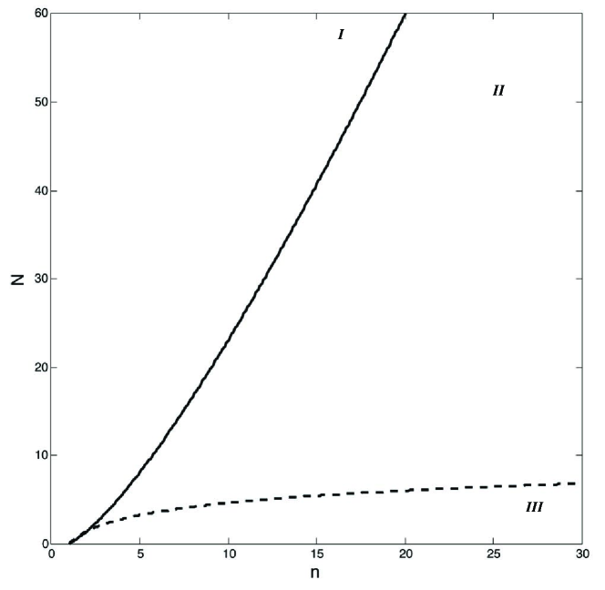
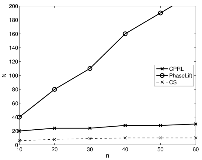
albeit the source signal was not assumed sparse. Using the lifting technique to construct the SDP relaxation of the NP-hard phase retrieval problem, with high probability, the program (20) recovers the exact solution (sparse or dense) if the number of measurements is at least of the order of . The region of success is visualized in Figure 1 as region I.
If is sufficiently sparse and random Fourier dictionaries are used for sampling, Moravec et al. [2007] showed that in general the signal is uniquely defined if the number of squared magnitude output measurements exceeds the order of . This lower bound for the region of success of CPR is illustrated by the dash line in Figure 1.
Finally, the motivation for introducing the -norm regularization in (16) is to be able to solve the sparse phase retrieval problem for smaller than what PhaseLift requires. However, one will not be able to solve the compressive phase retrieval problem in region III below the dashed curve. Therefore, our target problems lie in region II.
Example 1 (Compressive Phase Retrieval).
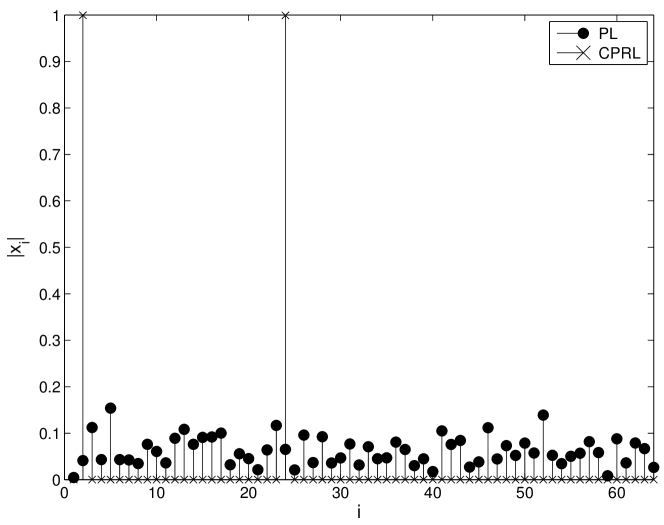
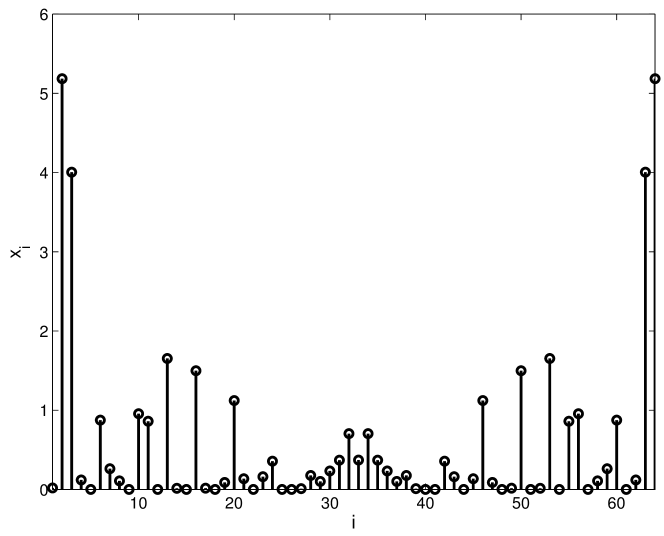
In this example, we illustrate a simple CPR example, where a 2-sparse complex signal is first transformed by the Fourier transform followed by random projections (generated by sampling a unit complex Gaussian):
| (21) |
Given , , and , we first apply PhaseLift algorithm Candès et al. [2011c] with to the squared observations . The recovered dense signal is shown in Figure 2. As seen in the figure, PhaseLift fails to identify the 2-sparse signal.
Next, we apply CPRL (24), and the recovered sparse signal is also shown in Figure 2. CPRL correctly identifies the two nonzero elements in .
3 Stable Numerical Solutions for Noisy Data
In this section, we consider the case that the measurements are contaminated by data noise. In a linear model, typically bounded random noise affects the output of the system as , where is a noise term with bounded -norm: . However, in phase retrieval, we follow closely a more special noise model used in Candès et al. [2011c]:
| (22) |
This nonstandard model avoids the need to calculate the squared magnitude output with the added noise term. More importantly, in practical phase retrieval applications, measurement noise is introduced when the squared magnitudes or intensities of the linear system are measured, not on itself (Candès et al. [2011c]).
Accordingly, we denote a linear operator of as
| (23) |
which measures the noise-free squared output. Then the approximate CPR problem with bounded error model (22) can be solved by the following SDP program:
| (24) |
The estimate of , just as in noise free case, can finally be found by computing the rank-1 decomposition of via singular value decomposition. We refer to the method as approximate CPRL. Due to the machine rounding error, in general a nonzero should be always assumed in the objective (24) and its termination condition during the optimization.
We should further discuss several numerical issues in the implementation of the SDP program. The constrained CPRL formulation (24) can be rewritten as an unconstrained objective function:
| (25) |
where and are two penalty parameters.
In (25), due to the lifting process, the rank-1 condition of is approximated by its trace function . In Candès et al. [2011c], the authors considered phase retrieval of generic (dense) signal . They proved that if the number of measurements obeys for a sufficiently large constant , with high probability, minimizing (25) without the sparsity constraint (i.e. ) recovers a unique rank-1 solution obeying . See also Recht et al. [2010].
In Section 7, we will show that using either random Fourier dictionaries or more general random projections, in practice, one needs much fewer measurements to exactly recover sparse signals if the measurements are noise free. Nevertheless, in the presence of noise, the recovered lifted matrix may not be exactly rank-1. In this case, one can simply use its rank-1 approximation corresponding to the largest singular value of .
We also note that in (25), there are two main parameters and that can be defined by the user. Typically is chosen depending on the level of noise that affects the measurements . For associated with the sparsity penalty , one can adopt a warm start strategy to determine its value iteratively. The strategy has been widely used in other sparse optimization, such as in -min [Yang et al., 2010]. More specifically, the objective is solved iteratively with respect to a sequence of monotonically decreasing , and each iteration is initialized using the optimization results from the previous iteration. The procedure continues until a rank 1 solution has been found. When is large, the sparsity constraint outweighs the trace constraint and the estimation error constraint, and vice versa.
Example 2 (Noisy Compressive Phase Retrieval).
Let us revisit Example 1 but now assume that the measurements are contaminated by noise. Using exactly the same data as in Example 1 but adding uniformly distributed measurement noise between and , CPRL was able to recover the 2 nonzero elements. PhaseLift, just as in Example 1 gave a dense estimate of .
4 Computational Aspects
In this section we discuss computational issus of the proposed SDP formulation, algorithms for solving the SDP and to efficient approximative solution algorithms.
4.1 A Greedy Algorithm
Since (16) is an SDP, it can be solved by standard software, such as CVX [Grant and Boyd, 2010]. However, it is well known that the standard toolboxes suffer when the dimension of is large. We therefore propose a greedy approximate algorithm tailored to solve (16). If the number of nonzero elements in is expected to be low, the following algorithm may be suitable and less computationally heavy compare to approaching the original SDP:
Example 3 (GCPRL ability to solve the CPR problem).
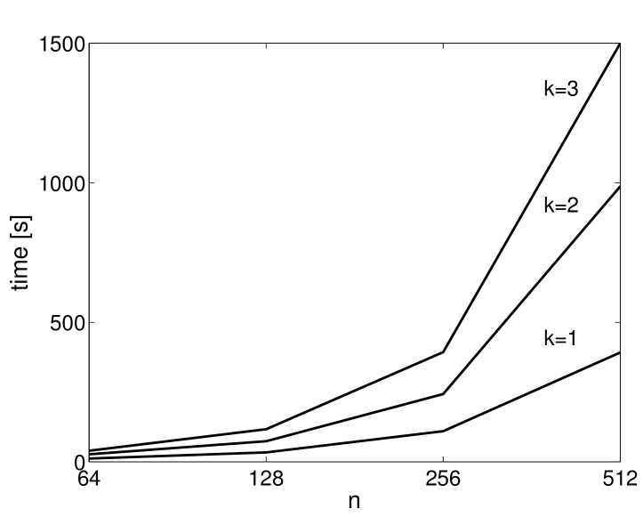
To demonstrate the effectiveness of GCPRL let us consider a numerical example. Let the true be a -sparse signal, let the nonzero elements be randomly chosen and their values randomly distributed on the complex unit circle. Let be generated by sampling from a complex unit Gaussian distribution.
If we fix , that is, twice as many unknowns as measurements, and apply GCPRL for different values of and we obtain the computational times visualized in the left plot of Figure 3. In all simulations and are used in GCPRL. The true sparsity pattern was always recovered. Since GCPRL can be executed in parallel, the simulation times can be divided by the number of cores used (the average run time in Figure 3 is computed on a standard laptop running Matlab, 2 cores, and using CVX to solve the low dimensional SDP of GCPRL). The algorithm is several magnitudes faster than the standard interior-point methods used in CVX.
5 The Dual
CPRL takes the form:
| (29) |
If we define to be an -dimensional vector such that our constraints are , then we can equivalently write:
| (33) |
Then the dual becomes:
| (37) |
6 Analysis
This section contains various analysis results. The analysis follows that of CS and have been inspired by derivations given in [Candès et al., 2011c, 2006, Donoho, 2006, Candès, 2008, Berinde et al., 2008, Bruckstein et al., 2009]. The analysis is divided into four subsections. The three first subsections give results based on RIP, RIP-1 and mutual coherency respectively. The last subsection focuses on the use of Fourier dictionaries.
6.1 Analysis Using RIP
In order to state some theoretical properties, we need a generalization of the restricted isometry property (RIP).
Definition 4 (RIP).
We will say that a linear operator is -RIP if for all s.t. we have
| (38) |
We can now state the following theorem:
Theorem 5 (Recoverability/Uniqueness).
Let be a -RIP linear operator with and let be the sparsest solution to (4). If satisfies
| (39) | ||||
then is unique and .
Proof of Theorem 5.
Assume the contrary i.e., . It is clear that and hence . If we now apply the RIP inequality (38) on and use that we are led to the contradiction . We therefore conclude that is unique and . ∎
We can also give a bound on the sparsity of :
Theorem 6 (Bound on from above).
Proof of Theorem 6.
Corollary 7 (Guaranteed Recovery Using RIP).
Proof of Corollary 7.
This follows trivially from Theorem 5 by realizing that satisfy all properties of .
∎
If can not be guaranteed, the following bound could come useful:
Theorem 8 (Bound on ).
Let and assume to be a -RIP linear operator. Let be any matrix (sparse or dense) satisfying
| (40) | ||||
let be the CPRL solution, (16), and form from by setting all but the largest elements to zero, i.e.,
| (41) |
Then,
| (42) |
with .
Proof of Theorem 8.
The proof is inspired by the work on compressed sensing presented in Candès [2008].
First, we introduce . For a matrix and an index set , we use the notation to mean the matrix with all zeros except those indexed by , which are set to the corresponding values of . Then let be the index set of the largest elements of in absolute value, and be its complement. Let be the index set associated with the largest elements in absolute value of and be the union. Let be the index set associated with the largest elements in absolute value of , and so on.
Notice that
| (43) |
We will now study each of the two terms on the right hand side separately.
We first consider . For we have that for each and that . Hence . Therefore,
| (44) |
and
| (45) |
Now, since minimizes , we have
| (46) |
Hence,
| (47) |
Using the fact , we get a bound for :
| (48) |
Subsequently, the bound for is given by
| (49) | ||||
| (50) |
Next, we consider . It can be shown by a similar derivation as in Candès [2008] that
| (51) |
Lastly, combine the bounds for and , and we get the final result:
| (52) | ||||
| (53) | ||||
| (54) | ||||
| (55) |
∎
The bound given in Theorem 8 is rather impractical since it contains both and . The weaker bound given in the following corollary does not have this problem:
Corollary 9 (A Practical Bound on ).
The bound on in Theorem 8 can be relaxed to a weaker bound:
| (56) | ||||
| (57) |
If is -sparse, , and is an -RIP linear operator, then we can guarantee that if
| (58) |
and has rank 1.
6.2 Analysis Using RIP-1
We define RIP-1 as follows:
Definition 10 (RIP-1).
A linear operator is -RIP-1 if for all matrices subject to , we have
| (67) |
Theorems 5–6 and Corollary 7 all hold with RIP replaced by RIP-1. The proofs follow those of the previous section with minor modifications (basically replace the 2-norm with the -norm). The RIP-1 counterparts of Theorems 5–6 and Corollary 7 are not restated in details here. Instead we summarize the most important property in the following theorem:
Theorem 11 (Upper Bound & Recoverability Through ).
6.3 Analysis Using Mutual Coherence
The RIP type of argument may be difficult to check for a given matrix and are more useful for claiming results for classes of matrices/linear operators. For instance, it has been shown that random Gaussian matrices satisfy the RIP with high probability. However, given one sample of a random Gaussian matrix, it is hard to check if it actually satisfies the RIP or not.
Two alternative arguments are spark Chen et al. [1998] and mutual coherence Donoho and Elad [2003], Candès et al. [2011b]. The spark condition usually gives tighter bounds but is known to be difficult to compute. On the other hand, mutual coherence may give less tight bounds, but is more tractable. We will focus on mutual coherence here.
Mutual coherence is defined as:
Definition 12 (Mutual Coherence).
For a matrix , define the mutual coherence as
| (68) |
By an abuse of notation, let be the matrix satisfying with being the vectorized version of . We are now ready to state the following theorem:
Theorem 13 (Recovery Using Mutual Coherence).
7 Experiment
This section gives a number of comparisons with the other state-of-the-art methods in compressive phase retrieval. Code for the numerical illustrations can be downloaded from http://www.rt.isy.liu.se/~ohlsson/code.html.
7.1 Simulation
First, we repeat the simulation given in Example 1 for . For each , is fixed, and we increase the measurement dimension until CPRL recovered the true sparse support in at least 95 out of 100 trials, i.e., 95% success rate. New data (, , and ) are generated in each trial. The curve of 95% success rate is shown in Figure 4.
With the same simulation setup, we compare the accuracy of CPRL with the PhaseLift approach and the CS approach in Figure 4. First, note that CS is not applicable to phase retrieval problems in practice, since it assumes the phase of the observation is also given. Nevertheless, the simulation shows CPRL via the SDP solution only requires a slightly higher sampling rate to achieve the same success rate as CS, even when the phase of the output is missing. Second, similar to the discussion in Example 1, without enforcing the sparsity constraint in (20), PhaseLift would fail to recover correct sparse signals in the low sampling rate regime.
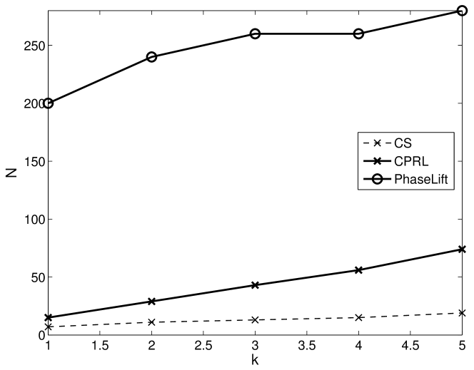
It is also interesting to see the performance as and vary and held fixed. We therefore use the same setup as in Figure 4 but now fixed and for gradually increased until CPRL recovered the true sparsity pattern with 95% success rate. The same procedure is repeated to evaluate PhaseLift and CS. The results are shown in Figure 5.
Compared to Figure 4, we can see that the degradation from CS to CPRL when the phase information is omitted is largely affected by the sparsity of the signal. More specifically, when the sparsity is fixed, even when the dimension of the signal increases dramatically, the number of squared observations to achieve accurate recovery does not increase significantly for both CS and CPRL.
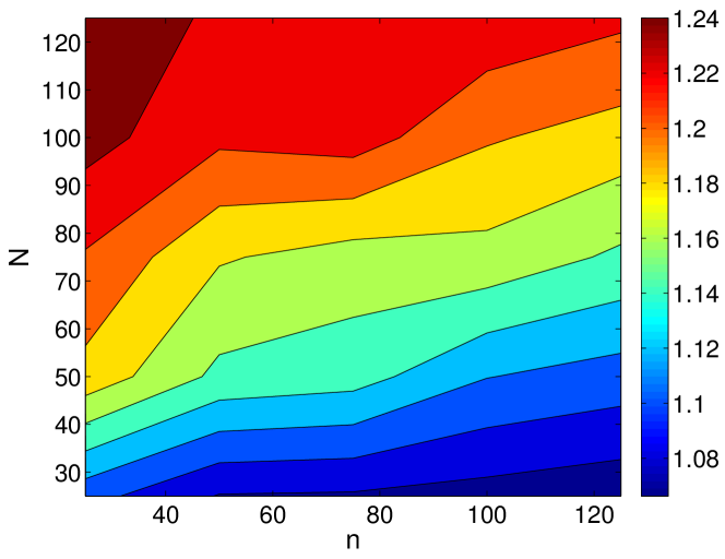
Next, we calculate the quantity , as Theorem 13 shows that when
| (70) |
and has rank 1, then . The quantity is plotted for a number of different and ’s in Figure 6. From the plot it can be concluded that if the solution has rank 1 and only a single nonzero component for a choice of , Theorem 13 can guarantee that . We also observer that Theorem 13 is pretty conservative, since from Figure 5 we have that with high probability we needed to guarantee that a two sparse vector is recovered correctly for .
7.2 Audio Signals
In this section, we further demonstrate the performance of CPRL using signals from a real-world audio recording. The timbre of a particular note on an instrument is determined by the fundamental frequency, and several overtones. In a Fourier basis, such a signal is sparse, being the summation of a few sine waves. Using the recording of a single note on an instrument will give us a naturally sparse signal, as opposed to synthesized sparse signals in the previous sections. Also, this experiment will let us analyze how robust our algorithm is in practical situations, where effects like room ambience might color our otherwise exactly sparse signal with noise.
Our recording is a real signal, which is assumed to be sparse in a Fourier basis. That is, for some sparse , we have , where is a matrix representing a transform from Fourier coefficients into the time domain. Then, we have a randomly generated mixing matrix with normalized rows, , with which our measurements are sampled in the time domain:
| (71) |
Finally, we are only given the magnitudes of our measurements, such that .
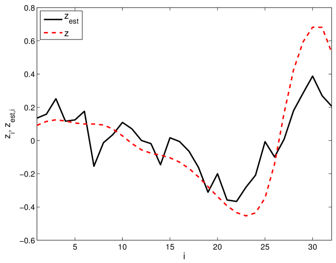
For our experiment, we choose a signal with samples, measurements, and it is represented with (overcomplete) Fourier coefficients. Also, to generate , the matrix representing the Fourier transform is generated, and rows from this matrix are randomly chosen.
The experiment uses part of an audio file recording the sound of a tenor saxophone. The signal is cropped so that the signal only consists of a single sustained note, without silence. Using CPRL to recover the original audio signal given , , and , the algorithm gives us a sparse estimate , which allows us to calculate . We observe that all the elements of have phases that are apart, allowing for one global rotation to make purely real. This matches our previous statements that CPRL will allow us to retrieve the signal up to a global phase.
We also find that the algorithm is able to achieve results that capture the trend of the signal using less than measurements. In order to fully exploit the benefits of CPRL that allow us to achieve more precise estimates with smaller errors using fewer measurements relative to , the problem should be formulated in a much higher ambient dimension. However, using the CVX Matlab toolbox by Grant and Boyd [2010], we already ran into computational and memory limitations with the current implementation of the CPRL algorithm. These results highlight the need for a more efficient numerical implementation of CPRL as an SDP problem.
8 Conclusion and Discussion
A novel method for the compressive phase retrieval problem has been presented. The method takes the form of an SDP problem and provides the means to use compressive sensing in applications where only squared magnitude measurements are available. The convex formulation gives it an edge over previous presented approaches and numerical illustrations show state of the art performance.
One of the future directions is improving the speed of the standard SDP solver, i.e., interior-point methods, currently used for the CPRL algorithm. The authors have previously introduced efficient numerical acceleration techniques for -min [Yang et al., 2010] and Sparse PCA [Naikal et al., 2011] problems. We believe similar techniques also apply to CPR. Such accelerated CPR solvers would facilitate exploring a broad range of high-dimensional CPR applications in optics, medical imaging, and computer vision, just to name a few.
9 Acknowledgement
Ohlsson is partially supported by the Swedish foundation for strategic research in the center MOVIII, the Swedish Research Council in the Linnaeus center CADICS, the European Research Council under the advanced grant LEARN, contract 267381, and a postdoctoral grant from the Sweden-America Foundation, donated by ASEA’s Fellowship Fund. Sastry and Yang are partially supported by an ARO MURI grant W911NF-06-1-0076. Dong is supported by the NSF Graduate Research Fellowship under grant DGE 1106400, and by the Team for Research in Ubiquitous Secure Technology (TRUST), which receives support from NSF (award number CCF-0424422).
References
- Balan et al. [2006] R. Balan, P. Casazza, and D. Edidin. On signal reconstruction without phase. Applied and Computational Harmonic Analysis, 20:345–356, 2006.
- Beck and Teboulle [2009] A. Beck and M. Teboulle. A fast iterative shrinkage-thresholding algorithm for linear inverse problems. SIAM Journal on Imaging Sciences, 2(1):183–202, 2009.
- Berinde et al. [2008] R. Berinde, A.C. Gilbert, P. Indyk, H. Karloff, and M.J. Strauss. Combining geometry and combinatorics: A unified approach to sparse signal recovery. In Communication, Control, and Computing, 2008 46th Annual Allerton Conference on, pages 798–805, September 2008.
- Bruckstein et al. [2009] A. Bruckstein, D. Donoho, and M. Elad. From sparse solutions of systems of equations to sparse modeling of signals and images. SIAM Review, 51(1):34–81, 2009.
- Candès [2008] E. J. Candès. The restricted isometry property and its implications for compressed sensing. Comptes Rendus Mathematique, 346(9–10):589–592, 2008.
- Candès and Wakin [2008] E. J. Candès and M. Wakin. An introduction to compressive sampling. Signal Processing Magazine, IEEE, 25(2):21–30, March 2008.
- Candès et al. [2006] E. J. Candès, J. Romberg, and T. Tao. Robust uncertainty principles: Exact signal reconstruction from highly incomplete frequency information. IEEE Transactions on Information Theory, 52:489–509, February 2006.
- Candès et al. [2011a] E. J. Candès, Y. Eldar, T. Strohmer, and V. Voroninski. Phase retrieval via matrix completion. Technical Report arXiv:1109.0573, Stanford Univeristy, September 2011a.
- Candès et al. [2011b] E. J. Candès, X. Li, Y. Ma, and J. Wright. Robust Principal Component Analysis? Journal of the ACM, 58(3), 2011b.
- Candès et al. [2011c] E. J. Candès, T. Strohmer, and V. Voroninski. PhaseLift: Exact and stable signal recovery from magnitude measurements via convex programming. Technical Report arXiv:1109.4499, Stanford Univeristy, September 2011c.
- Chai et al. [2010] A. Chai, M. Moscoso, and G. Papanicolaou. Array imaging using intensity-only measurements. Technical report, Stanford University, 2010.
- Chen et al. [1998] S. Chen, D. Donoho, and M. Saunders. Atomic decomposition by basis pursuit. SIAM Journal on Scientific Computing, 20(1):33–61, 1998.
- Dainty and Fienup [1987] J. Dainty and J. Fienup. Phase retrieval and image reconstruction for astronomy. In Image Recovery: Theory and Applications. Academic Press, New York, 1987.
- d’Aspremont et al. [2007] A. d’Aspremont, L. El Ghaoui, M. Jordan, and G. Lanckriet. A direct formulation for Sparse PCA using semidefinite programming. SIAM Review, 49(3):434–448, 2007.
- Donoho [2006] D. Donoho. Compressed sensing. IEEE Transactions on Information Theory, 52(4):1289–1306, April 2006.
- Donoho and Elad [2003] David L. Donoho and Michael Elad. Optimally sparse representation in general (nonorthogonal) dictionaries via l-minimization. PNAS, 100(5):2197–2202, March 2003.
- Fienup [1982] J. Fienup. Phase retrieval algorithms: a comparison. Applied Optics, 21(15):2758–2769, 1982.
- Fienup [1987] J. Fienup. Reconstruction of a complex-valued object from the modulus of its Fourier transform using a support constraint. Journal of Optical Society of America A, 4(1):118–123, 1987.
- Gerchberg and Saxton [1972] R. Gerchberg and W. Saxton. A practical algorithm for the determination of phase from image and diffraction plane pictures. Optik, 35:237–246, 1972.
- Gonsalves [1976] R. Gonsalves. Phase retrieval from modulus data. Journal of Optical Society of America, 66(9):961–964, 1976.
- Grant and Boyd [2010] M. Grant and S. Boyd. CVX: Matlab software for disciplined convex programming, version 1.21. http://cvxr.com/cvx, August 2010.
- Hoerl and Kennard [1970] A. Hoerl and R. Kennard. Ridge regression: Biased estimation for nonorthogonal problems. Technometrics, 12(1):55–67, 1970.
- Kohler and Mandel [1973] D. Kohler and L. Mandel. Source reconstruction from the modulus of the correlation function: a practical approach to the phase problem of optical coherence theory. Journal of the Optical Society of America, 63(2):126–134, 1973.
- Loris [2009] I. Loris. On the performance of algorithms for the minimization of -penalized functionals. Inverse Problems, 25:1–16, 2009.
- Marchesini [2007] S. Marchesini. Phase retrieval and saddle-point optimization. Journal of the Optical Society of America A, 24(10):3289–3296, 2007.
- Millane [1990] R. Millane. Phase retrieval in crystallography and optics. Journal of the Optical Society of America A, 7:394–411, 1990.
- Moravec et al. [2007] M. Moravec, J. Romberg, and R. Baraniuk. Compressive phase retrieval. In SPIE International Symposium on Optical Science and Technology, 2007.
- Naikal et al. [2011] N. Naikal, A. Yang, and S. Sastry. Informative feature selection for object recognition via sparse PCA. In Proceedings of the 13th International Conference on Computer Vision (ICCV), 2011.
- Recht et al. [2010] B. Recht, M. Fazel, and P Parrilo. Guaranteed minimum-rank solutions of linear matrix equations via nuclear norm minimization. SIAM Review, 52(3):471–501, 2010.
- Tibsharani [1996] R. Tibsharani. Regression shrinkage and selection via the lasso. Journal of Royal Statistical Society B (Methodological), 58(1):267–288, 1996.
- Tropp [2004] J. Tropp. Greed is good: Algorithmic results for sparse approximation. IEEE Transactions on Information Theory, 50(10):2231–2242, October 2004.
- Walther [1963] A. Walther. The question of phase retrieval in optics. Optica Acta, 10:41–49, 1963.
- Yang et al. [2010] A. Yang, A. Ganesh, Y. Ma, and S. Sastry. Fast -minimization algorithms and an application in robust face recognition: A review. In ICIP, 2010.