Fast Algorithms for Sparse Recovery with Perturbed Dictionary

Abstract

In this paper, we account for approaches of sparse recovery from large underdetermined linear models with perturbation present in both the measurements and the dictionary matrix. Existing methods have high computation and low efficiency. The total least-squares (TLS) criterion has well-documented merits in solving linear regression problems while FOCal Underdetermined System Solver (FOCUSS) has low-computation complexity in sparse recovery. Based on TLS and FOCUSS methods, the present paper develops more fast and robust algorithms, TLS-FOCUSS and SD-FOCUSS. TLS-FOCUSS algorithm is not only near-optimum but also fast in solving TLS optimization problems under sparsity constraints, and thus fit for large scale computation. In order to reduce the complexity of algorithm further, another suboptimal algorithm named SD-FOCUSS is devised. SD-FOCUSS can be applied in MMV (multiple-measurement-vectors) TLS model, which fills the gap of solving linear regression problems under sparsity constraints. The convergence of TLS-FOCUSS algorithm and SD-FOCUSS algorithm is established with mathematical proof. The simulations illustrate the advantage of TLS-FOCUSS and SD-FOCUSS in accuracy and stability, compared with other algorithms.

I Introduction

The problem of finding sparse solutions to underdetermined system of linear equations has been a hot spot of researches in recent years, because of its widespread application in compressive sensing/sampling (CS)[1, 2], biomagnetic imagining[3], source localization [4], signal reconstruction[5, 6], etc.

In the noise-free setup, CS theory holds promise to explain the equivalence between $\ell_{0}$-norm minimization and $\ell_{1}$-norm minimization as solving exactly linear equations when the unknown vector is sparse[7, 8]. Variants of CS for ”noise setup” of perturbed measurements are usually solved based on basis pursuit (BP) approach[9, 10] (utilizing method of linear programming[4] or Lasso[11]), greedy algorithms (e.g. OMP[12], ROMP[13], CoSaMP[14], etc) or least-squares methods with $\ell_{1}$-regularization (e.g., FOCUSS[5, 15, 6]). However, exiting BP, greedy algorithms and FOCUSS do not account for perturbations present in the dictionary matrix, i.e. regression matrix.

Recently, only a little attention has been paid on the sparse problems with perturbations present both in measurements and dictionary matrix. Performance analysis of CS and BP methods for the linear regression model under sparsity constraints was researched in [16], [17] and [18]; a feasible approach in [19] , named S-TLS, was devised to reconstruct sparse vectors based on Lasso from the ”fully-perturbed” linear model. However, the research of [16], [17] and [18] are limited in theoretical aspect and do not devise systematic approaches. Due to its highly-computational burden, S-TLS is very time-consuming, and thus unsuitable for large scale problems.

In this paper, an extension form of FOCUSS is devised solving sparse problems to ”fully-perturbed” linear model. Belonging to categories of convex optimization, LP and Lasso have the stable results but their computational burden is the highest; greedy algorithms have low computation, but their performances can only be guaranteed when the dictionary matrix satisfies some rigorous conditions, such as very small restricted isometry constants [7]. FOCUSS was originally designed to obtain a sparse solution by successively solving quadratic optimization problems and was widely used to deal with compressed sensing problems. The obvious advantages of FOCUSS are its low computation and stable results. For FOCUSS, only a few iterations tends to be enough to obtain a rather good approximating solution. So it is an excellent choice to develop FOCUSS to solve approximate sparse solutions to linear regression model, especially in large scale application.

Our objective is to overcome the influence of perturbation present in dictionary matrix and measurements on the accuracy of sparse recovery effectively. Meanwhile, the merits of FOCUSS, rapid convergence and good adaption to intrinsic properties of dictionary matrix, are maintained. First, objective function to be optimized can be obtained under a Bayesian framework. Then the necessary condition for the optimizing solution is that each first-order partial derivative of objective function is equal to zero. Next we can get the iterative expression using iterative relaxation algorithm. Finally, the new algorithms are proved to be convergent.

The paper is organized as follows. In Section II, we introduce perturbed linear regression model for sparse recovery, and analyze the optimal problem simply. In Section III, we use a MAP estimate to obtain the objective function to be optimized, then yield an iterative algorithm to provide solutions, named TLS-FOCUSS for adopting TLS method and framework of FOCUSS. Convergence of TLS-FOCUSS is proved. In Section IV, we propose another algorithm based on FOCUSS and TLS model, named SD-FOCUSS to distinguish TLS-FOCUSS. Though SD-FOCUSS is a suboptimal optimal, its computation is low and it can be used in MMV case. In the simulation of Section V, the performances of mentioned algorithms are presented. Finally, we draw some conclusions in Section VI.

II Perturbed Linear Regression Model

Consider the underdetermined linear system of $\textbf{y}=A\textbf{x}$, where $A$ is an $m\times n$ matrix with $m<n$, y is the given $m\times 1$ data vector, and x is unknown $n\times 1$ vector to be recovered. With x being sparse, and $A$ satisfying some property (e.g., RIP[7]), CS theory asserts that exact recovery of x can be guaranteed by solving the convex problem[9, 7, 20]: $\min_{x}\|\textbf{x}\|_{1}~{}~{}\textrm{s.t.}(\textrm{subject~{}to})~{}\textbf{y}=A\textbf{x}$. Suppose that data perturbations exist in the linear model $A\textbf{x}$. The corresponding convex problem can be written as a Lagrangian form[9, 4, 15]: $\min_{\textbf{x}}\|\textbf{y}-A\textbf{x}\|_{2}^{2}+\gamma\|\textbf{x}_{p}^{p}$, where $\|\cdot\|_{p}^{p}=\sum|\cdot|^{p}$, $\gamma>0$ is a sparsity-tuning parameter[19], and $0<p\leq 1$ ($p$ is set to 1 in [9, 19]). What the present paper focusses on is how to reconstruct sparse vector efficiently from over- and especially under-determined linear regression models while perturbations are present in y and/or $A$.

The perturbed linear regression model can be formulated as follows[21, 22]:

$$\textbf{y}=(A+E)\textbf{x}+\textbf{e},$$ (1)

where e represents perturbation vector and $E$ represents perturbation matrix. Due to randomness and uncertainty, it is usually assumed that the components of noise in the same channel are independently and identically Gaussian distributed, e.g. $\textbf{e}\sim N(0,\sigma_{1}^{2}I)$ and $\textrm{vec}(E)\sim N(0,\sigma_{2}^{2}I)$, where vec$(\cdot)$ is matrix vectorizing operator.

(1) can be rewritten as

$$(B+D)\left[{\begin{array}[]{*{20}{c}}{1}\\ {\textbf{x}}\end{array}}\right]=0,$$

where $B=[-\textbf{y},A],{\quad}D=[\textbf{e},E]$. Without exploiting sparsity, TLS has well documented merits solving above problem. For over-determined models TLS estimates are given by

$$\hat{\textbf{x}}=\arg\min_{D,\textbf{x}}\|D\|_{F}^{2},\quad\textrm{s.t.}(B+D)\left[\begin{array}[]{c}1\\ \textbf{x}\end{array}\right]=0,$$

where $\|\cdot\|_{F}^{2}$ represents Forbenius-form operator. With the assumption of $\textrm{vec}(D)\sim N(0,\sigma^{2})$, [22] gives the equivalent solutions as

$$\hat{\textbf{x}}=\arg\min_{\textbf{x}}\frac{\|\textbf{y}-A\textbf{x}\|^{2}}{1+\|\textbf{x}\|^{2}}$$ (2)

The distinct objective of the present paper is twofold: developing efficient solvers for fully-perturbed linear models, and accounting for sparsity of x. To achieve these goals, following optimization problem must be sovled

$$\hat{\textbf{x}}=\arg\min_{\textbf{x},D}\left[\|D\|_{F}^{2}+\gamma\|\textbf{x}\|_{p}^{p}\right],$$ (3)

where $\gamma>0$, and $0<p\leq 1$. In (3), the $\ell_{F}$-term forces the quadratic sum of perturbations to be minimal while the $\ell_{p}$-term forces sparsity of recovery[9, 19], and $\gamma$ controls tradeoff between above two terms. Developing efficient algorithms to get the local even global optimum of (3) is the main goal. In next section, we will explain how to get the objective function and estimate the value of $\gamma$ with a bayesian formation, then develop the new method of optimization.

III TLS-FOCUSS Algorithm

This section develops an extension of FOCUSS, TLS-FOCUSS, to solve (1) using Bayesian framework [9] and main idea of TLS. For simplifying formulas, we assume $\sigma=\sigma_{1}=\sigma_{2}$, that is $\textrm{vec}(D)\sim N(0,\sigma^{2})$. At the end of the section, we will introduce how to process the situation with $\sigma_{1}\neq\sigma_{2}$.

III-A Bayesian Formulation

From (1), we obtain

$$\textbf{y}-A\textbf{x}=G(\textbf{x})\textbf{v},$$ (4)

where $G(\textbf{x})=[1,\textbf{x}^{T}]\otimes{I_{m\times{m}}}$, $\textbf{v}=\textrm{vec}(D)$, ($\otimes$ represents Kronecker product). Under Bayesian viewpoint, unknown vector x is assumed to be random and independent of $D$. Then the MAP estimation of x can be obtained as:

$$\hat{\textbf{x}}_{\textrm{MAP}} =\arg\max_{\textbf{x}}\ln{p(\textbf{x}|\textbf{y})}$$

$$=\arg\max_{\textbf{x}}[\ln{p(\textbf{y}|\textbf{x})}+\ln{p(\textbf{x})}].$$ (5)

This formula is general and offers considerable flexibility. In order to obtain optimality of the resultant estimates, another assumption must be made on the distributions of the solution vector x. As discussed in [15], the elements of sparse x are assumed to be distributed as general Gaussian and independent,

$$p(\textbf{x})=C_{2}\exp\left(-\frac{1}{2\beta^{p}}\sum_{k=1}^{m}\big{|}\textbf{x}[k]\big{|}^{p}\right),$$ (6)

where $C_{2}$ is constant, $0<p\leq 1$ and $\beta$ is constant depended on $p$ with $\beta=2^{-\frac{p}{2}}\frac{\Gamma(1/p)}{\Gamma(3/p)}$ ( where $\Gamma(\cdot)$ means Gamma function). Only one parameter characterizes the distribution in (6). The pdf moves toward a uniform distribution as $p\to\infty$ and toward a very peaky distribution as $p\to 0$.

With $\textbf{v}{\sim}N(0,\sigma^{2}I)$ and $G(\textbf{x})G^{H}(\textbf{x})=(1+\|\textbf{x}\|^{2})I$, we have

$$\ln{p(\textbf{y}|\textbf{x})}=\frac{1}{2\sigma^{2}}\frac{(\textbf{y}-A\textbf{x})^{H}(\textbf{y}-A\textbf{x})}{1+\|\textbf{x}\|^{2}}+C_{1},$$ (7)

where $C_{1}$ is constant. With the densities of the perturbation vector v and the solution vector x, we can now proceed to find the MAP estimate as

$$\hat{\textbf{x}}_{\textrm{MAP}}=\arg\min_{\textbf{x}}\left[\frac{\|\textbf{y}-A\textbf{x}\|_{2}^{2}}{1+\|\textbf{x}\|_{2}^{2}}+\gamma\|\textbf{x}\|_{p}^{p}\right],$$ (8)

where $\gamma=\sigma^{2}/\beta^{p}$.

III-B Derivation of TLS-FOCUSS

The optimization problem (8) is equivalent to

$$\begin{array}[]{c}\arg\min_{\textbf{z}^{\prime}}J(\textbf{z}^{\prime})\\ \textrm{where}\quad J(\textbf{z}^{\prime})=\left[\frac{\|B\textbf{z}^{\prime}\|_{2}^{2}}{\|\textbf{z}^{\prime}\|_{2}^{2}}+\gamma\|\textbf{z}^{\prime}\|_{p}^{p}\right],\end{array}$$ (11)

with

$$\textbf{z}^{\prime}=\left[\begin{array}[]{c}1\\ \textbf{x}\end{array}\right],{\quad}B=[-\textbf{y},A].$$ (12)

To simplify the objective function,we normalize $\textbf{z}^{\prime}$ and get the equivalent form as

$$\min_{\textbf{z}}\left[\left\|B\textbf{z}\right\|_{2}^{2}+\gamma\left\|\textbf{z}\right\|_{p}^{p}\right],\quad\textrm{s.t.}\ \|\textbf{z}\|_{2}^{2}=1.$$ (13)

Using Lagrange multiplier method, the objective function can be rewritten as

$$T(\textbf{z})=\|B\textbf{z}\|_{2}^{2}+\gamma\|\textbf{z}\|_{p}^{p}+\lambda(1-\textbf{z}^{H}\textbf{z}),$$ (14)

where $\lambda$ is the Lagrange multiplier. The factored gradient approach developed in [23], an iterative method can be derived to minimize $T(\textbf{z}$. A necessary condition for the optimum solution $\textbf{z}_{*}$ is that it must satisfy $\nabla_{z}T(\textbf{z}_{*})=0$. We can get

$$(B^{H}B+\alpha\Pi(\textbf{z}_{*}))\textbf{z}_{*} =\lambda\textbf{z}_{*},$$ (15)

where

$$\alpha=p\gamma/2,{\quad}\Pi(\textbf{z})=\textrm{diag}\left(\left[\left|\textbf{z}[i]\right|^{p-2}\right]_{i=1,\cdots,n+1}\right).$$

So the iterative relaxation scheme can be constructed as

$$\big{(}B^{H}B+\alpha\Pi(\textbf{z}_{k-1})\big{)}\textbf{z}_{k}=\lambda\textbf{z}_{k}.$$ (16)

It is easily seen that $\lambda$ should be the minimal eigenvalue of objective matrix $B^{H}B+\alpha\Pi(\textbf{z}_{k-1})$. However, it’s very hard to find it for two reasons: firstly, the minimal eigenvalue is likely close to zero because objective matrix is approximately singular; secondly, the dimension of matrix above is tremendous for most large scale application, which leads to a big computational burden for matrix inversion. (16) implies that

$$\big{(}B^{H}B+\alpha\Pi(\textbf{z}_{k-1})\big{)}^{-1}\textbf{z}_{k}=\frac{1}{\lambda}\textbf{z}_{k}.$$ (17)

From (17), finding the minimal eigenvalue is taken place of by finding the maximal eigenvalue. The latter become much more well-posed. Moreover, with the aid of matrix inversion formula, we have

$$\big{(}B^{H}B+\alpha\Pi(\textbf{z}_{k-1})\big{)}^{-1}$$

$$= \frac{1}{\alpha}\Big{(}W_{k}^{2}-W_{k}^{2}B^{H}\big{(}\alpha{I}-BW_{k}^{2}B^{H}\big{)}^{-1}BW_{k}^{2}\Big{)},$$ (18)

where $W_{k}^{2}=\Pi^{-1}(\textbf{z}_{k-1})$. Let

$$\Phi_{k}=W_{k}^{2}-W_{k}^{2}B^{H}(\alpha{I}-BW_{k}^{2}B^{H})^{-1}BW_{k}^{2},$$ (19)

then we obtain

$$\Phi_{k}\textbf{z}_{k}=\frac{\alpha}{\lambda}\textbf{z}_{k}.$$ (20)

It should be mentioned that the dimension of matrix $\alpha{I}-BW_{k}^{2}B^{H}$ is much less than that of matrix $B^{H}B+\alpha\Pi(\textbf{z}_{k-1})$, so the cost of matrix inversion is extremely reduced. Besides, we need only calculate the maximal eigenvalue and corresponding eigenvector instead of all the eigenvalue and eigenvector of $\Phi_{k}$. That is to say, some highly efficient solver, such as Lanczos iteration, could be utilized to make the problem further simplified.

Noting that the optimal problem (8) is not global convex, the TLS-FOCUSS algorithm guarantees convergence to a local optimum. Once the initial point $\textbf{z}_{0}$ is close to the true point, estimation of true value can be found through iterations. In this paper, we set $\textbf{x}_{0}=A^{H}(AA^{H})^{-1}\textbf{y}$, then $\textbf{z}_{0}$ is set through substituting $\textbf{x}_{0}$ into (12) and normalization of $\textbf{z}_{0}^{\prime}$.

When the convergent solution $\textbf{z}_{*}$ is obtained, we can get

$$\ \textbf{x}_{TLS-FOCUSS}=[z_{*2},\cdots,z_{*{n+1}}]^{T}/z_{*1}.$$ (21)

Algorithm 1 is the algorithmic description of TLS-FOCUSS.

Algorithm 1 (TLS-FOCUSS)

• Input: $\textbf{z}_{0}$, $B$, $\alpha$, $p$.

• Set $W_{k}=\textrm{diag}\left(\left[\left|\textbf{z}_{k-1}[i]\right|^{1-\frac{p}{2}}\right]_{i=1,\cdots,n+1}\right)($, and $p\in(0,1]$);

• Calculate $\Phi_{k}=W_{k}^{2}-W_{k}^{2}B^{H}(\alpha{I}+BW_{k}^{2}B^{H})^{-1}BW_{k}^{2}$.

• Compute the largest eigenvalue $\lambda_{k}$ and corresponding eigenvector $\textbf{u}_{k}$ of $\Phi_{k}$ using Lanczos method.

• Set $\textbf{z}_{k}=\textbf{u}_{k}$.

• If $\|\textbf{z}_{k}-\textbf{z}_{k-1}\|_{2}^{2}/\|\textbf{z}_{k-1}\|_{2}^{2}<\epsilon$, exit; else goto step 1.

III-C Convergence and Sparsity

To show that TLS-FOCUSS algorithm can approximately solve the sparse problem of (1) through iterative method, two key results should be obtained: i) TLS-FOCUSS is a convergent algorithm that it indeed reduces $J(\textbf{z})$ at each iterate step; ii) the convergence points of TLS-FOCUSS are sparse.

Proof:

From (16) we have

$$B_{W}^{H}B_{W}\textbf{q}_{k}+\alpha\textbf{q}_{k}-\lambda W_{k}^{2}\textbf{q}_{k}=0,$$ (22)

where $B_{W}=BW_{k}$, $\textbf{q}_{k}=W^{-1}_{k}\textbf{z}_{k}$. And $\textbf{q}_{k}$ can be treated as an optimal solution:

$$\textbf{q}_{k}=\arg\min_{\textbf{q}}\left[\|B_{W}\textbf{q}\|^{2}+\alpha\|\textbf{q}\|^{2}+\lambda(1-\textbf{q}^{H}W_{k}^{2}\textbf{q})\right].$$ (23)

From (23) and the equivalence of optimization between (11) and (14), $\textbf{z}_{k}$ can be expressed a solution to an optimization problem:

$$\textbf{z}_{k}= \arg\min Q_{k}(\textbf{z}),$$

$$\textrm{where}~{}Q_{k}(\textbf{z})= \frac{\|B\textbf{z}\|^{2}}{\|\textbf{z}\|^{2}}+\alpha\|W_{k}^{-1}\textbf{z}\|^{2}.$$ (24)

So TLS-FOCUSS algorithm can be considered to be a method of re-weighted $\ell_{2}$-form minimization [5, 15]. Since $\textbf{z}_{k}$ is the local unique solution to minimize $Q_{k}(\textbf{z})$, we have

$$Q_{k}(\textbf{z}_{k})<Q_{k}(\textbf{z}_{k-1})$$ (25)

with $\textbf{z}_{k},~{}\textbf{z}_{k-1}$ located in the same small domain and $\textbf{z}_{k}\neq\textbf{z}_{k-1}$.

And we can get the conclusion [15] that

$$\sum_{i}\left(|{z}_{2}[i]|^{p}-|{z}_{1}[i]|^{p}\right)$$

$$\leq \sum_{i}\frac{p}{2}|z_{1}[i]|^{p-2}\left(z_{2}[i]^{2}-z_{1}[i]^{2}\right)$$

$$= \frac{p}{2}\left[\textbf{z}_{2}^{T}\Pi(\textbf{z}_{1})\textbf{z}_{2}-\textbf{z}_{1}^{T}\Pi(\textbf{z}_{1})\textbf{z}_{1}\right],$$ (26)

where $\Pi(\textbf{z})=diag(|z[i]|^{p-2})$. With $\textbf{z}_{k-1}$ and $\textbf{z}_{k}$ ($\textbf{z}_{k}\neq\textbf{z}_{k-1}$) obtained from the $(k-1)$th and $k$th iteration of TLS-FOCUSS, we have

$$J(\textbf{z}_{k})-J(\textbf{z}_{k-1})$$

$$\leq \left[{\frac{\|B\mathbf{z}_{k}\|_{2}^{2}}{\|\mathbf{z}_{k}\|_{2}^{2}}+{\alpha\mathbf{z}_{k}^{T}W_{k}^{-2}\mathbf{z}_{k}}}\right]-\left[{\frac{\|B\textbf{z}_{k-1}\|_{2}^{2}}{\|\textbf{z}_{k-1}\|_{2}^{2}}+{\alpha\mathbf{z}_{k-1}^{T}W_{k}^{-2}\mathbf{z}_{k-1}}}\right]$$

$$= Q_{k}(\textbf{z}_{k})-Q_{k}(\textbf{z}_{k-1})<0,$$ (27)

where $\textbf{z}_{k}$ and $\textbf{z}_{k-1}$ are obtained from the $k\textrm{-th}$ and ($k-1$)-th iteration step of TLS-FOCUSS. The first inequality follows from (III-C) and the last inequality from (25). So the value of $J(\textbf{z}_{k})$ decreases as $k$ increases. From (III-C) and $J(\textbf{z}_{k})\geq 0$, it can be concluded that TLS-FOCUSS is a convergent algorithm. ∎

Proof:

Assuming $\textbf{z}_{0}$ is a local minima of $J(\textbf{z})$, $\textbf{z}_{0}$ is also a local minima to an optimization problem: $\min\limits_{\textbf{z}}\sum\limits_{i}|z[i]|^{p}\quad\textrm{s.t.}~{}(B+D)\textbf{z}=0$, which can be rewritten as

$$\min_{\textbf{x}}\sum_{i}\left|x[i]\right|^{p}\quad\textrm{s.t.}~{}\textbf{y}=(A+E)\textbf{x}+\textbf{e}.$$ (28)

Similarly shown in [4, 15, 24] (especially $p=1$), as an equivalence of $\ell_{0}$-norm optimization above optimization problem can obtain the local minima which are necessary sparse. The provement of equivalence between $\ell_{0}$-norm and $\ell_{p}$-norm about fully-perturbed model is aslo an open problem.

Let $\textbf{z}_{*}$ be an fixed point of the algorithm, and therefore a solution of (17). If $\textbf{z}_{*}$ is not sparse, it is not a local minima of (28), so there must be other points close to $\textbf{z}_{*}$ which can reduce $J(\textbf{z})$[23]. Thus it can be concluded that only sparse solutions are stable points of TLS-FOCUSS algorithm. ∎

III-D Robust Modification

Note that we assumed the components of perturbation matrix $[\textbf{e},E]$ are i.i.d. (independent and identically distributed). Actually, only noise existing in the same channel is assumed to be i.i.d.. When e and $E$ have the different distributed variances, it is necessary to normalize variances of perturbations before signal reconstruction. Assume that e and $E$ are independent, and $\textbf{e}\sim N(0,\sigma^{2}I_{1})$, $\textrm{vec}(E)\sim N(0,\sigma_{2}^{2}I_{2})$. Then we have $\textbf{y}-A\textbf{x}=G(\textbf{x})\textbf{v}$ with

$$G(\textbf{x})=\left[1,\frac{\sigma_{2}}{\sigma}\textbf{x}^{T}\right]\otimes{I_{m\times{m}}},~{}\textbf{v}=\left[\begin{array}[]{c}\textbf{e}\\ \frac{\sigma}{\sigma_{2}}\textrm{vec}(E).\end{array}\right]$$

It can be seen $\textbf{v}\sim N(0,\sigma^{2}I)$. For (11), instead of (12) we have

$$\textbf{z}^{\prime}=[1,\frac{\sigma_{2}}{\sigma}\textbf{x}^{T}]^{T},{\quad}B=[-\textbf{y},\frac{\sigma}{\sigma_{2}}A].$$

Now TLS-FOCUSS algorithm can be used to recover the sparse signal.

IV SD-FOCUSS Algorithm

TLS-FOCUSS needs to compute the maximal eigenvalue and its corresponding eigenvector of matrix $\Phi_{k}$ in every iteration. By utilizing Lanczos algorithm, TLS-FOCUSS algorithm can be speeded up greatly. However, it is still possible to release much more the computation burden while the performance descends a little. In this section, a suboptimal algorithm, named SD-FOCUSS (Synchronous Descending FOCUSS), is divised.

Based on TLS model (1), Zhu in [19] devised a sparse recovery algorithm S-TLS. To optimize the objective function, S-TLS adopted iterative block coordinate descent method, yielding successive estimates of x with $E$ fixed and alternately of $E$ with x fixed until obtaining stable solutions. The algorithm needs several convergent procedures before final convergence. Different from S-TLS, SD-FOCUSS is more efficient, which only needs one convergent procedure, with estimating x and $E$ synchronously in each iteration; meanwhile, SD-FOCUSS has lower computation complexity.

IV-A Bayesian Formulation

In this section, x and $E$ in (1) are both considered variants to be optimized. Assume that $e\sim N(0,\sigma^{2}I_{1})$, $\textrm{vec}(E)\sim N(0,\sigma_{2}^{2}I_{2})$, and $e$, $E$ are independent. So we have

$$p_{\textbf{e}}(\textbf{e}) =C_{3}\exp\left(-\frac{\textbf{e}^{H}\textbf{e}}{2\sigma_{1}^{2}}\right)$$

$$p_{E}({E}) =C_{4}\exp\left(-\frac{\textrm{vec}({E})^{H}\textrm{vec}({E})}{2\sigma_{2}^{2}}\right)=\exp\left(-\frac{\|{E}\|_{F}^{2}}{2\sigma_{2}^{2}}+C_{2}\right)$$ (29)

Where $C_{1}$, $C_{2}$ are constant. The Bayesian formulation is described as

$$[\hat{\textbf{x}}_{\textrm{MAP}},\hat{E}_{\textrm{MAP}}]=\arg\max_{\textbf{x},E}\ln p(\textbf{x},E|\textbf{y})$$

$$= \arg\max_{\textbf{x},E}\left[\ln p(\textbf{y}|\textbf{x},E)+\ln p(\textbf{x})+\ln p(E)\right].$$ (30)

Here we have

$$\ln p(\textbf{y}|\textbf{x},E)=\frac{1}{\sigma_{1}^{2}}\left\|\textbf{y}-\left(A+E\right)\textbf{x}\right\|_{2}^{2}+\ln C_{3}.$$ (31)

IV-B Derivation of SD-FOCUSS

From (6) (IV-A) and (31), the objective function can be written as

$$J(\textbf{x},E)=\left\|\textbf{y}-\left(A+E\right)\textbf{x}\right\|_{2}^{2}+\frac{\sigma^{2}}{\sigma_{2}^{2}}\textrm{tr}(E^{H}E)+\gamma\|\textbf{x}\|_{p}^{p}$$ (32)

where $\textrm{tr}(\cdot)$ means trace of matrix and $\textrm{tr}(E^{H}E)=\|E\|_{F}^{2}$. The necessary condition of the optimal solution satisfies that partial differentiation to each component for $J(\textbf{x},E)$ is equal to zero, that is:

a) $\nabla_{E}J(x,E_{*})=0$.

We can get

$$\nabla_{E}J(\textbf{x},E)=E{\textbf{x}}\textbf{x}^{H}-(\textbf{y}-A\textbf{x})\textbf{x}^{H}+\sigma_{1}^{2}\sigma_{2}^{-1}E.$$

So we can get the estimate of $E$ as a function of x:

$${E_{*}(\textbf{x})}=\frac{(\textbf{y}-A\textbf{x})\textbf{x}^{H}}{\sigma_{1}^{2}\sigma_{2}^{-2}+\textbf{x}^{H}\textbf{x}}.$$ (33)

Here the fact of $(\lambda I+F^{H}F)^{-1}F^{H}=F^{H}(\lambda I+FF^{H})^{-1}$ is used.

b) $\nabla_{x}J(x_{*},E)=0$.

Referring to [15], we can get the iterative relaxation scheme of x as

$$\textbf{x}_{k}=W_{k}A_{k}^{H}(A_{k}A_{k}^{H}+\alpha I)^{-1}\textbf{y},$$ (34)

where $\alpha=\frac{p\gamma}{2}$, $W_{k}=\textrm{diag}\left(\left[|\textbf{x}_{k-1}[i]|^{1-\frac{p}{2}}\right]_{i=1,\cdots,n}\right)$ and $A_{k}=\big{(}A+E(\textbf{x}_{k-1})\big{)}W_{k}$. There exists error inevitably when we estimate $E$, thus accuracy of estimating x will be affected. It is a suboptimal algorithm.

Algorithm 2 is the algorithmic description of SD-FOCUSS.

Algorithm 2 (SD-FOCUSS)

• Input: $y$, $\textbf{x}_{0}$, $E_{0}$ $A$, $\sigma$, $\sigma_{2}$, $p$.

• Set $W_{k}=\textrm{diag}\left(\left[\left|\textbf{x}_{k-1}[i]\right|^{1-\frac{p}{2}}\right]_{i=1,\cdots,n}\right)($, and $p\in(0,1])$;

• Calculate

  $${E_{k}}=\frac{{({\bf{y}}-A{{\bf{x}}_{k-1}}){\bf{x}}_{k-1}^{H}}}{{{\sigma^{2}}\sigma_{2}^{-2}+\left\|{{{\bf{x}}_{k-1}}}\right\|_{2}^{2}}},~{}\textrm{and}~{}A_{k}=(A+E_{k})W_{k};$$

• Calculate $\textbf{x}_{k}=W_{k}A_{k}^{H}(A_{k}A_{k}^{H}+\alpha I)^{-1}\textbf{y}$;

• If $\|\textbf{x}_{k}-\textbf{x}_{k-1}\|_{2}^{2}/\|\textbf{x}_{k-1}\|_{2}^{2}<\epsilon$, exit; else goto step 1.

IV-C Proof of Convergence

Formula (34) can be seen as $\textbf{x}_{k}=W_{k}\textbf{b}_{k}$, where $\textbf{b}_{k}$ can be treated as an optimal solution, that is

$$\textbf{b}_{k}=\arg\min\|\textbf{y}-A_{k}W_{k}\textbf{b}\|_{2}^{2}+\alpha\|\textbf{b}\|_{2}^{2}$$ (35)

Alternately and equivalently, $\textbf{x}_{k}$ can be expressed a solution to an optimization problem:

$$\textbf{x}_{k} =\arg\min_{x}Q_{k}(\textbf{x}),$$

$$\textrm{where}\quad Q_{k}(\textbf{x}) =\|\textbf{y}-A_{k}\textbf{x}\|_{2}^{2}+\alpha\|W_{k}^{-1}\textbf{x}\|_{2}^{2}.$$ (36)

Referring to (25)-(III-C), we can conclude that SD-FOCUSS is also a convergent algorithm.

IV-D SD-FOCUSS Extension: MMV case

Besides low computation, the breakthrough advantage of SD-FOCUSS is that it can be used in multiple measurement vectors (MMV) model, while TLS-FOCUSS and S-TLS [19] cannot fit this model or remain to be developed. Supposed $\textbf{y}^{(l)}=(A+E)\textbf{x}^{(l)}+\textbf{e}^{(l)}$, with $l=1,\cdots,L$, where $\textbf{y}^{(l)}\in R^{m}$ and $\textbf{x}^{(l)}\in R^{n}$. Suppose that the vectors $\textbf{x}^{(l)},l=1,\cdots,L$ are sparse and have the same sparsity profile, and let $Y=[\textbf{y}^{(1)},\cdots,\textbf{y}^{(L)}]$, $X=[\textbf{x}^{(1)},\cdots,\textbf{x}^{(L)}]$.

The objective function for MMV case is expressed as

$$J(X,E)= \left\|Y-\left(A+E\right)X\right\|_{F}^{2}+$$

$$\frac{\sigma^{2}}{\sigma_{2}^{2}}\|E\|_{F}^{2}+\gamma\sum_{i=1}^{n}\left(\sum_{l=1}^{L}x^{(l)}[i]^{2}\right)^{p/2}$$ (37)

The weight matrix $W_{k}$ can be re-expressed as [6]

$$W_{k}= \textrm{diag}\left(c_{k}[i]^{1-p/2}\right)\quad\textrm{with}~{}c_{k}[i]=\left(\sum_{l=1}^{L}\big{(}x_{k-1}^{(l)}[i]\big{)}^{2}\right)^{1/2}$$ (38)

Then formula (34) can be rewritten as

$$X_{k}=W_{k}A_{k}^{H}(A_{k}A_{k}^{H}+\alpha I)^{-1}Y$$ (39)

For $\nabla_{E}J(x,E)=0$ we can renew (33) as

$$E_{k}=(Y-AX_{k-1})\left(\frac{\sigma^{2}}{\sigma_{2}^{2}}I+X_{k-1}^{H}X_{k-1}\right)^{-1}X_{k-1}^{H}$$ (40)

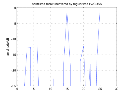
(a) Result recovered by Regularized FOCUSS: weak signal is loss

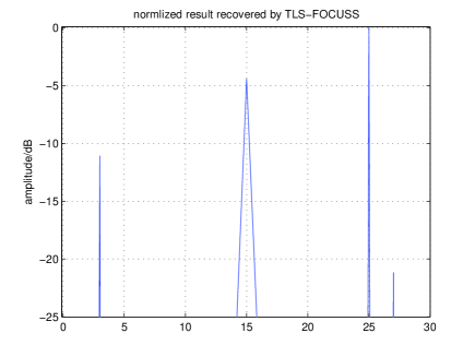
(b) Result of recovered by TLS-FOCUSS: weak signal is found

Figure 1: Result of weak signal recovery with $m=20,n=30$

Then the Algorithm 2 can be modified to fit MMV model as Algorithm 3.

Algorithm 3 (MMV SD-FOCUSS)

• Input: $y$, $\textbf{x}_{0}$, $E_{0}$ $A$, $\sigma$, $\sigma_{2}$, $p$.

• Set $W_{k}=\textrm{diag}\left(\left[c_{k}[i]^{1-\frac{p}{2}}\right]_{i=1,\cdots,n}\right)$,
  where $c_{k}[i]=\left(\sum_{l=1}^{L}\big{(}x_{k-1}^{(l)}[i]\big{)}^{2}\right)^{1/2}$, $p\in(0,1])$;

• Calculate

  $$E_{k}=(Y-AX_{k-1})\left[\sigma^{2}\sigma_{2}^{-2}I+X_{k-1}^{H}X_{k-1}\right]^{-1}X_{k-1}^{H}$$

  and $A_{k}=(A+E_{k})W_{k}$;

• Calculate $X_{k}=W_{k}A_{k}^{H}(A_{k}A_{k}^{H}+\alpha I)^{-1}Y$;

• If $\|X_{k}-X_{k-1}\|_{2}^{2}/\|X_{k-1}\|_{2}^{2}<\epsilon$, exit; else goto step 1.

V Simulation Results

The parameters in this paper are set as: norm-factor $p=0.5$, convergence threshold $\epsilon=0.01$. In each Monte Carlo simulation, 1000 trials are carried out independently. In each trial, the $m{\times}n$ dictionary $A$ is chosen as Gaussian random matrix, entries of which are independently, identically and normally distributed. In order to analyze the mentioned algorithms, the true sparse solution has to be known, and it is hard to know in practice problems.

The algorithm in one simulation is considered to be successful if all nonzero-locations of x are found exactly; otherwise, the algorithm is considered to be failed.

V-A Single Measurement Vector Case

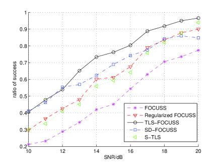
(a) success probability of algorithms in finding the support set correctly

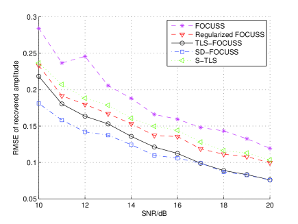
(b) RMSE of signal amplitude recovery

Figure 2: Performance of involved algorithms with $m=20,n=30$

This subsection shows the advantages of recovering ability of new algorithms from TLS model with numerical simulation. Let x be a $s$-sparse vector, i.e. $\|\textbf{x}\|_{0}=s$, and let the average power of x be normalized, i.e. $\sum_{i}{|x_{i}|^{2}}=1$. In each trial, entries of matrix $[e,E]$ are also independently and identically Gaussian distributed with mean zero and variance $\sigma^{2}$. Then overall SNR can be represented as $1/\sigma^{2}$. The indices of nonzero coordinate set $T$ are chosen randomly from a discrete uniform distribution $U(1,N)$ (without repetition).

In following simulations, besides TLS-FOCUSS and SD-FOCUSS, other algorithms will be involved: standard FOCUSS [5], Regularized FOCUSS [15], and S-TLS [19].

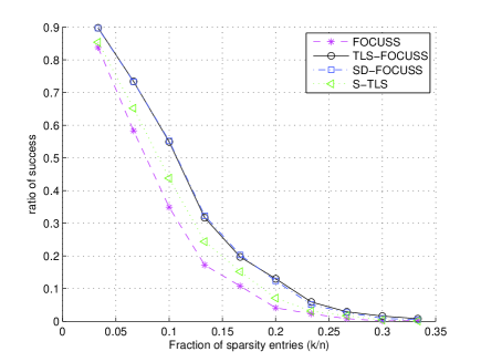
(a) percentage success with randiness distribution in sparse entries

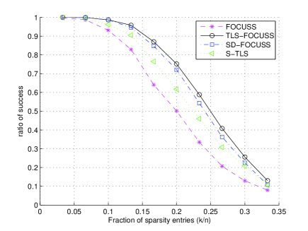
(b) percentage success with the same amplitude in sparse entries

Figure 3: percentage success of involved algorithms with different $k/m$. $m=20,n=30$

In Fig. 1 and Fig. 2, the number of rows and columns of dictionary matrix are set to 20 and 30 respectively. In Fig. 1, SNR is set to 15 dB, $T=[3,15,25]$ and $\textbf{x}_{T}=[0.4139,-0.9186,-1.4819]^{T}$. It can be seen from Fig. 1 that TLS-FOCUSS does much better than FOCUSS in extracting weak signal when dictionary and measurement are both corrupted. For TLS-FOCUSS, the position and amplitude of signal are both recovered excellently; the result of FOCUSS is failed, for weak signal is buried in ”False Peak” brought by perturbation on dictionary and can not be distinguished correctly. Fig. 2(A) shows the statistical results of percentage success, and Fig. 2(B) shows the statistical root-mean-square error (RMSE) of signal amplitude recovery when algorithms can find the nonzero-coordinate $T$ correctly under different SNR scenes. TLS-FOCUSS and SD-FOCUSS are presented to be more robust from Fig. 2(a), and perform much better on amplitude recovery from Fig. 2(b).

Fig. 3 shows the percentage-success curves of algorithms with different $k/m$. In the simulation, $m=20,~{}n=30,~{}k=1,2,\cdots,10$, SNR=15dB and entries of $\textbf{x}_{T}$ are set to obey i.i.d. normal distribution in Fig. 3(a) and 1 in Fig. 3(b). It can be seen from Fig. 3 that, TLS-FOCUSS and SD-FOCUSS perform always better than common algorithms (FOCUSS) and S-TLS designed to solve fully-perturbed model as $k/m$ changes.

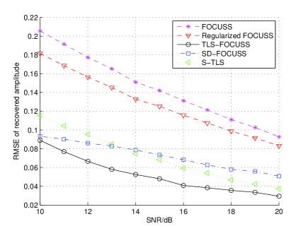
Figure 4: RMSE of signals recovery in the condition of $m=128$, $n=512$.

In the simulations of Fig. 4 and Table I, $m=128$, $n=512$, $s=3$ and $\textbf{x}_{T}=(1,-1,1)^{T}/\sqrt{3}$. With smooth curves, Fig. 4 shows that the recovery performance of TLS-FOCUSS in this scenario is much better than the other algorithms; SD-FOCUSS is superior to S-TLS in low SNR, and inferior to S-TLS in high SNR. Table I shows run-times of mentioned algorithms under the same condition. In order to obtain a measure of the computational complexity, the average CPU times for each algorithm consumeing is tabulated in Table I. It can be seen that, as the same classified algorithms TLS-FOCUSS and SD-FOCUSS are much faster than S-TLS.

By comparison with other algorithms, it can be concluded that TLS-FOCUSS and SD-FOCUSS have the complete advances in percentage succuss, accurate reconstruction and computational speed. And TLS-FOCUSS has the higher success percentage and more accurate reconstruction than SD-FOCUSS while SD-FOCUSS is faster than TLS-FOCUSS.

V-B MMV Case

In this simulation we consider the performance of SD-FOCUSS in MMV case. $X$ is a sparse matrix with $L$ columns and only $s$ rows with nonzero entries. In each trial, the indices of nonzero rows in $X$ are chosen randomly from a discrete uniform distribution, and the amplitudes of the row entries are generalized randomly from a standard normal distribution; entries of both $E$ and $[\textbf{e}^{(l)}]_{l=1,\cdots,L}$ are independently Gaussian distributed with mean zero and variance $\sigma^{2}$. The overall SNR is $1/\sigma^{2}$. The measurement matrix can expressed as

$$Y=(A+E)X+[\textbf{e}^{(l)}]_{l=1,\cdots,L}$$

The relative MSE between the true and estimate solution is defined as [6]

$$\textrm{MSE}=\textrm{E}\left(\frac{\|\hat{X}-X\|_{F}^{2}}{\|X\|_{F}^{2}}\right)$$

In following simulations, besides SD-FOCUSS, the other algorithms will be involved, containing: MMV FOCUSS [6], Regularized MMV FOCUSS [6], and MMV OMP [6].

SNR	FOCUSS	RegFOC	TLS-FOC	SD-FOC	S-TLS
(dB)	(sec)	(sec)	(sec)	(sec)	(sec)
10	0.1284	0.0160	0.5841	0.3008	5.1528
11	0.1298	0.0182	0.6530	0.3513	5.3670
12	0.1274	0.0185	0.6291	0.3276	5.3779
13	0.1218	0.0158	0.5852	0.3010	5.2276
14	0.1215	0.0156	0.6001	0.2964	5.2652
15	0.1211	0.0156	0.5863	0.2959	5.3563
16	0.1202	0.0155	0.5858	0.2961	5.3963
17	0.1213	0.0156	0.5867	0.2958	5.3639
18	0.1211	0.0155	0.5880	0.2966	5.3069
19	0.1213	0.0163	0.6104	0.3121	5.2285
20	0.1221	0.0156	0.5921	0.2965	5.1877

TABLE I: Run-time of algorithms with $m=128,n=512$. The simulations are done in Matlab 7.8 on a Core 2, 3.0-GHz, 2-GByte RAM PC

The number of rows and columns of dictionary $A$ are set to 20 and 30 respectively, and let $s=7$. Two quantities are varied in this experiment: SNR and $L$. Fig. 5 and Fig. 6 show success-probability curves and MSE curves respectively when $L=2,5,6$. It can be found that as $L$ becomes larger, success numbers become larger; however, MSE curves seem to be unchanged for it is related with perturbation and unrelated with $L$. MMV SD-FOCUSS performs better than other algorithms.

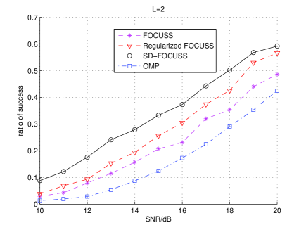
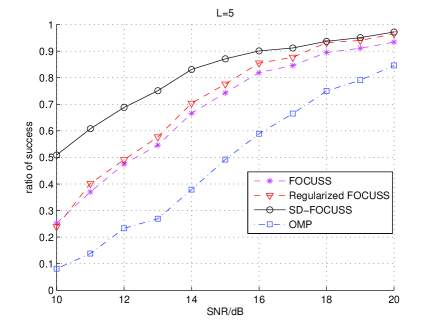
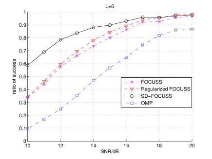
Figure 5: Success probability of algorithms obtaining all $s$ nonzero rows in MMV case, with $m=20,~{}n=30,~{}\textrm{s}=7$ and Number of observation vectors is set to $L=2,5,6$.

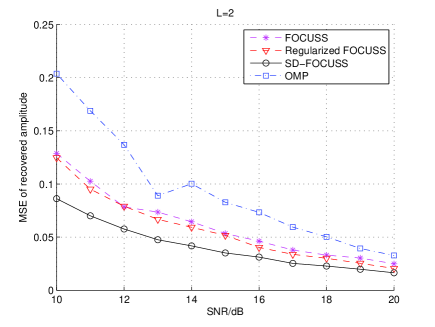
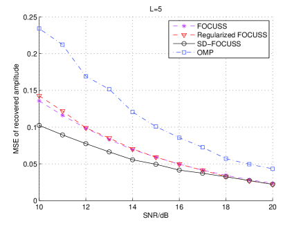
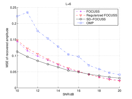
Figure 6: Relative MSE of amplitude recovery in MMV case, with $m=20,~{}n=30,~{}\textrm{s}=7$ and Number of observation vectors is set to $L=2,5,6$.

VI Conclusion

In this paper, through extending FOCUSS algorithms, we have proposed two new algorithms, TLS-FOCUSS and SD-FOCUSS, to recover the sparse vector from an underdetermined system when the measurements and dictionary matrix are both perturbed. The convergence of algorithms was considered. Then we applied SD-FOCUSS in MMV model with a row-sparsity structure. The simulations showed our approaches performed better than other present algorithms in computational complexity, percentage success and RMSE of signal amplitude recovery. The benefits of TLS-FOCUSS and SD-FOCUSS make them be good candidates of sparse recovery algorithms for more practical applications.

References

- [1] D. L. Donoho, “Compressed sensing,” IEEE Trans. on Inf. Theory, vol. 52, pp. 1289–1306, April 2006.
- [2] E. J. Candes, “Compressive sampling,” International Congress of Mathematicians, vol. 3, pp. 1433–1452, 2006.
- [3] I. F. Gorodnitsky, J. George, and B. D. Rao, “Neuromagnetic source imaging with focuss: A recursive weighted minimum norm algorithm,” Electroencephalogr. Clin. Neurophysiol., vol. 95, no. 4, pp. 231–251, Oct. 1995.
- [4] D. Malioutov, M. Cetin, and A. S. Willsky, “A sparse signal reconstruction perspective for source localization with sensor arrays,” IEEE Trans. Signal Process., vol. 53, pp. 3010–3022, Aug. 2005.
- [5] I. F. Gorodnitsky and B. D. Rao, “Sparse signal reconstructions from limited data using focuss: A re-weighted minimum norm algorithm,” IEEE Trans. Signal Process., vol. 45, pp. 600–616, March 1997.
- [6] S. F. Cotter, B. D. Rao, K. Engan, and K. Kreutz-Delgado, “Sparse solutions to linear inverse problems with multiple measurement vectors,” IEEE Trans. Signal Process., vol. 53, pp. 2477–2488, July 2005.
- [7] E. Candes and T. Tao, “Decoding by linear programming,” IEEE Trans. Inf. Theory, vol. 51, pp. 4203–4215, December 2005.
- [8] E. J. Candès, “The restricted isometry property and its implications for compressed sensing,” Comptes Rendus Mathematique, vol. 346, no. 9-10, pp. 589–592, Oct. 2008.
- [9] S. Chen, D. L. Donoho, and M. A. Saunders, “Atomic decomposition by basis pursuit,” SIAM J. Sci. Comput., vol. 20, pp. 33–61, 1998.
- [10] D. L. Donoho and X. Huo, “Uncertainty principles and ideal atomic decomposition,” IEEE Trans. on Inf. Theory, vol. 47, pp. 2845–2862, Novermber 2001.
- [11] R. Tibshirani, “Regression shrinkage and selection via the lasso,” J. Roy. Statist. Soc., vol. 58, pp. 267–288, 1996.
- [12] J. A. Troppb and A. C. Gilbert, “Signal recovery from random measurements via orthogonal matching pursuit,” IEEE Trans. Inf. Theory, vol. 53, no. 12, pp. 4655–4666, 2007.
- [13] D. Needell and R. Vershynin, “Signal recovery from incomplete and inaccurate measurements via regularized orthogonal matching pursuit,” IEEE J. Selected Topics Signal Process., vol. 4, pp. 310–316, 2010.
- [14] D. Needell and J. A. Troppb, “Cosamp: Iterative signal recovery from incomplete and inaccurate samples,” Appl. Comput. Harmon. Anal., vol. 26, pp. 301–321, 2009.
- [15] B. D. Rao, K. Engan, S. F. Cotter, J. Palmer, and K. Kreutz-Delgado, “Subset selection in noise based on diversity measure minimization,” IEEE Trans. Signal Process., vol. 51, pp. 760–770, March 2003.
- [16] M.A. Herman and T. Strohmer, “General deviants: An analysis of perturbations in compressed sensing,” IEEE Journal of Selected Topics in Signal Process., vol. 4, pp. 342–349, April 2010.
- [17] D. H. Chae, P. Sadeghi, and R. A. Kennedy, “Effects of basis-mismatch in compressive sampling of continuous sinusoidal signals,” in Proc. of 2nd Intl. Conf. on Future Computer and Communication, May. 21-24 2010.
- [18] Y. Chi, A. Pezeshki, L. Scharf, and R. Calderbank, “Sensitivity to basis mismatch in compressed sensing,,” Mar. 14-19. 2010.
- [19] H. Zhu, G. Leus, and G. B. Giannakis, “Sparsity-cognizant total least-squares for perturbed compressive sampling,” IEEE Trans. Signal Process., vol. 59, pp. 2002–2016, 2011.
- [20] E. J. Candes, “The restricted isometry property and its implications for compressed sensing,” Comptes Rendus Mathematique, vol. 346, no. 9-10, pp. 589–592, 2008.
- [21] G. H. Golub and C. F. Van Loan, “An analysis of the total least squares problem,” SIAM J. Numer. Anal., vol. 17, pp. 883–893, December 1980.
- [22] X. Zhang, Matrix analysis and applications, Tsinghua Univ. Press, Bejing, 2004.
- [23] B. D. Rao and K. Kreutz-Delgado, “An affine scaling methodology for best basis selection,” IEEE Trans. Signal Processing, vol. 47, pp. 187–200, Jan. 1999.
- [24] E. J. Candès, J. K. Romberg, and T. Tao, “Stable signal recovery from incomplete and inaccurate measurements,” Comm. Pure Appl. Math., vol. 59, pp. 1207–1223, 2006.