A rigorous model study of the adaptative dynamics of Mendelian diploids.

Abstract

Adaptive dynamics so far has been put on a rigorous footing only for clonal inheritance. We extend this to sexually reproducing diploids, although admittedly still under the restriction of an unstructured population with Lotka-Volterra-like dynamics and single locus genetics (as in Kimura’s 1965 infinite allele model). We prove under the usual smoothness assumptions, starting from a stochastic birth and death process model, that, when advantageous mutations are rare and mutational steps are not too large, the population behaves on the mutational time scale (the ’long’ time scale of the literature on the genetical foundations of ESS theory) as a jump process moving between homozygous states (the trait substitution sequence of the adaptive dynamics literature). Essential technical ingredients are a rigorous estimate for the probability of invasion in a dynamic diploid population, a rigorous, geometric singular perturbation theory based, invasion implies substitution theorem, and the use of the Skorohod $M_{1}$ topology to arrive at a functional convergence result. In the small mutational steps limit this process in turn gives rise to a differential equation in allele or in phenotype space of a type referred to in the adaptive dynamics literature as ’canonical equation’.

MSC 2000 subject classification: 92D25, 60J80, 37N25, 92D15, 60J75

Key-words: individual-based mutation-selection model, invasion fitness for diploid populations, adaptive dynamics, canonical equation, polymorphic evolution sequence, competitive Lotka-Volterra system.

1 Introduction

Adaptive dynamics (AD) aims at providing an ecology-based framework for scaling up from the micro-evolutionary process of gene substitutions to meso-evolutionary time scales and phenomena (also called long term evolution in papers on the foundations of ESS theory, that is, meso-evolutionary statics, cf Eshel (1983, in press); Eshel, Feldman, and Bergman (1998); Eshel and Feldman (2001)). One of the more interesting phenomena that AD has brought to light is the possibility of an emergence of phenotypic diversification at so-called branching points, without the need for a geographical substrate Metz et al. (1996); Geritz et al. (1998); Doebeli and Dieckmann (2000). This ecological tendency may in the sexual case induce sympatric speciation Dieckmann and Doebeli (1999). However, a population subject to mutation limitation and initially without variation stays essentially uni-modal, closely centered around a type that evolves continuously, as long as it does not get in the neighborhood of a branching point. In this paper we focus on the latter aspect of evolutionary trajectories.

AD was first developed, in the wake of Hofbauer and Sigmund (1987); Marrow, Law and Cannings (1992); Metz, Nisbet and Geritz (1992), as a systematic framework at a physicist level of rigor by Diekmann and Law Dieckmann and Law (1996) and by Metz and Geritz and various coworkers Metz, Nisbet and Geritz (1992); Metz et al. (1996); Geritz et al. (1998). The first two authors started from a Lotka-Volterra style birth and death process while the intent of the latter authors was more general, so far culminating in Durinx, Metz and Meszéna (2008). The details for general physiologically structured populations were worked out at a physicist level of rigor in Durinx, Metz and Meszéna (2008) while the theory was put on a rigorous mathematical footing by Champagnat and Méléard and coworkers Champagnat, Ferrière and Méléard (2008); Champagnat (2006); Méléard and Tran (2009), and recently also from a different perspective by Peter Jagers and coworkers Klebaner et al. (2011). All these papers deal only with clonal models. In the meantime a number of papers have appeared that deal on a heuristic basis with special models with Mendelian genetics (e.g. Kisdi and Geritz (1999); Van Dooren (1999, 2000); Van Doorn and Dieckmann (2006); Proulx and Phillips (2006); Peischl and Bürger (2008)), while the general biological underpinning for the ADs of Mendelian populations is described in Metz (in press). In the present paper we outline a mathematically rigorous approach along the path set out in Champagnat, Ferrière and Méléard (2008); Champagnat (2006), with proofs for those results that differ in some essential manner between the clonal and Mendelian cases. It should be mentioned though that just as in the special models in Kisdi and Geritz (1999); Van Dooren (1999, 2000); Proulx and Phillips (2006); Peischl and Bürger (2008) and contrary to the treatment in Metz (in press) we deal still only with the single locus infinite allele case (cf Kimura Kimura (1965)), while deferring the infinite loci case to a future occasion.

Our reference framework is a diploid population in which each individual’s ability to survive and reproduce depends only on a quantitative phenotypic trait determined by its genotype, represented by the types of two alleles on a single locus. Evolution of the trait distribution in the population results from three basic mechanisms: heredity, which transmits traits to new offsprings thus ensuring the extended existence of a trait distribution, mutation, generating novel variation in the trait values in the population, and selection acting on these trait values as a result of trait dependent differences in fertility and mortality. Selection is made frequency dependent by the competition of individuals for limited resources, in line with the general ecological spirit of AD. Our goal is to capture in a simple manner the interplay between these different mechanisms.

2 The Model

We consider a Mendelian population and a hereditary trait that is determined by the two alleles on but a single locus with many possible alleles (the infinite alleles model of Kimura Kimura (1965)). These alleles are characterized by an allelic trait $u$. Each individual $i$ is thus characterized by its two allelic trait values $(u^{i}_{1},u^{i}_{2})$, hereafter referred to as its genotype, with corresponding phenotype $\phi(u^{i}_{1},u^{i}_{2})$, with $\phi:\mathbb{R}^{m}\rightarrow\mathbb{R}^{n}$. In order to keep the technicalities to a minimum we shall below proceed on the assumption that $n=m=1$. In the Discussion we give a heuristic description of how the extension to general $n$ and $m$ can be made. When we are dealing with a fully homozygous population we shall refer to its unique allele as $A$ and when we consider but two co-circulating alleles we refer to these as $A$ and $a$.

We make the standard assumptions that $\phi$ and all other coefficient functions are smooth and that there are no parental effects, so that $\phi(u_{1},u_{2})=\phi(u_{2},u_{1})$, which has as immediate consequence that if $u_{a}=u_{A}+\zeta$, $|\zeta|\ll 1$, then $\phi(u_{A},u_{a})=\phi(u_{A},u_{A})+\partial_{2}\phi(u_{A},u_{A})\zeta+\mathrm{O}(\zeta^{2})$ and $\phi(u_{a},u_{a})=\phi(u_{A},u_{A})+2\partial_{2}\phi(u_{A},u_{A})\zeta+\mathrm{O}(\zeta^{2})$, i.e., the genotype to genotype map is locally additive, $\phi(u_{A},u_{a})\approx\left(\phi(u_{A},u_{A})+\phi(u_{a},u_{a})\right)/2$, and the same holds good for all quantities that smoothly depend on the phenotype.

Remark 2.1

The biological justification for the above assumptions is that the evolutionary changes that we consider are not so much changes in the coding regions of the gene under consideration as in its regulation. Protein coding regions are in general preceded by a large number of relatively short regions where all sorts of regulatory material can dock. Changes in these docking regions lead to changes in the production rate of the gene product. Genes are more or less active in different parts of the body, at different times during development and under different micro-environmental conditions. The allelic type $u$ should be seen as a vector of such expression levels. The genotype to phenotype map $\phi$ maps these expression levels to the phenotypic traits under consideration. It is also from this perspective that we should judge the assumption of smallness of mutational steps $\zeta$: the influence of any specific regulatory site among its many colleagues tends to be relatively minor.

The individual-based microscopic model from which we start is a stochastic birth and death process, with density-dependence through additional deaths from ecological competition, and Mendelian reproduction with mutation. We assume that the population’s size scales with a parameter $K$ tending to infinity while the effect of the interactions between individuals scales with ${1\over K}$. This allows taking limits in which we count individuals weighted with ${1\over K}$. As an interpretation think of individuals that live in an area of size $K$ such that the individual effects get diluted with area, e.g. since individuals compete for living space, with each individual taking away only a small fraction of the total space, the probability of finding a usable bit of space is proportional to the relative frequency with which such bits are around.

2.1 Model setup

The allelic trait space ${\cal U}$ is assumed to be a closed and bounded interval of $\mathbb{R}$. Hence the phenotypic trait space is compact. For any $(u_{1},u_{2})\in{\cal U}^{2}$, we introduce the following demographic parameters, which are all assumed to be smooth functions of the allelic traits and thus bounded. Moreover, these parameters are assumed to depend in principle on the allelic traits through the intermediacy of the phenotypic trait. Since the latter dependency is symmetric, we assume that all coefficient functions defined below are symmetric in the allelic traits.

$f(u_{1},u_{2})\in\mathbb{R}_{+}$

: the per capita birth rate (fertility) of an individual with genotype $(u_{1},u_{2})$.

$D(u_{1},u_{2})\in\mathbb{R}_{+}$

: the background death rate of an individual with genotype $(u_{1},u_{2})$.

$K\in\mathbb{N}$

: a parameter scaling the per capita impact on resource density and through that the population size.

$\frac{C((u_{1},u_{2}),(v_{1},v_{2}))}{K}\in\mathbb{R}_{+}$

: the competitive effect felt by an individual with genotype $(u_{1},u_{2})$ from an individual with genotype $(v_{1},v_{2})$. The function $C$ is customarily referred to as competition kernel.

$\mu_{K}\in\mathbb{R}_{+}$: the mutation probability per birth event (assumed to be independent of the genotype). The idea is that $\mu_{K}$ is made appropriately small when we let $K$ increase.

$\sigma>0$: a parameter scaling the mutation amplitude.

$m_{\sigma}(u,h)dh={1\over\sigma}m(u,{h\over\sigma})dh$: the mutation law of a mutant allelic trait $\,u+h$ from an individual with allelic trait $u$, with $m(u,h)dh$ a probability measure with support $[-1,1]\cap\{h\,|\,u+h\in{\cal U}\}$. As a result the support of $m_{\sigma}$ is of size $\leq 2\sigma$.

Notational convention: When only two alleles $A$ and $a$ co-circulate, we will use the shorthand:

$$f_{AA}=f(u_{A},u_{A})\ ;\ f_{Aa}=f(u_{A},u_{a})\ ;\ f_{aa}=f(u_{a},u_{a})\ ;\ D_{AA}=D(u_{A},u_{A})\ ;$$

$$C((u_{A},u_{a}),(u_{A},u_{A}))=C_{Aa,AA};\;\;\mathrm{etc.}$$

To keep things simple we take our model organisms to be hermaphrodites which in their female role give birth at rate $f$ and in their male role have probabilities proportional to $f$ to act as the father for such a birth.

We consider, at any time $t\geq 0$, a finite number $N_{t}$ of individuals, each of them with genotype in ${\cal U}^{2}$. Let us denote by $(u^{1}_{1},u^{1}_{2}),\ldots,(u_{1}^{N_{t}},u_{2}^{N_{t}})$ the genotypes of these individuals. The state of the population at time $t\geq 0$, rescaled by $K$, is described by the finite point measure on ${\cal U}^{2}$

$$\nu^{\sigma,K}_{t}={1\over K}\sum_{{i=1}}^{N_{t}}\delta_{(u^{i}_{1},u^{i}_{2})},$$ (2.1)

where $\delta_{(u_{1},u_{2})}$ is the Dirac measure at $(u_{1},u_{2})$.

Let $\langle\nu,g\rangle$ denote the integral of the measurable function $g$ with respect to the measure $\nu$ and $\mathrm{Supp}(\nu)$ the support of the latter. Then $\>\langle\nu^{\sigma,K}_{t},{\bf 1}\rangle=\frac{N_{t}}{K}$ and for any $(u_{1},u_{2})\in{\cal U}^{2}$, the positive number $\langle\nu^{\sigma,K}_{t},{\bf 1}_{\{(u_{1},u_{2})\}}\rangle$ is called the density at time $t$ of genotype $(u_{1},u_{2})$.

Let ${\cal M}_{F}$ denote the set of finite nonnegative measures on ${\cal U}^{2}$, equipped with the weak topology, and define

$${\cal M}^{K}=\left\{\frac{1}{K}\sum_{i=1}^{n}\delta_{(u_{1}^{i},u_{2}^{i})}:n\geq 0,\ (u^{1}_{1},u^{1}_{2}),\ldots,(u^{n}_{1},u^{n}_{2})\in{\cal U}^{2}\right\}.$$

An individual with genotype $(u_{1},u_{2})$ in the population $\nu^{\sigma,K}_{t}$ reproduces with an individual with genotype $(u^{j}_{1},u^{j}_{2})$ at a rate $f(u_{1},u_{2}){f(u^{j}_{1},u^{j}_{2})\over K\langle\nu^{\sigma,K},f\rangle}$.

With probability $1-\mu_{K}(u_{1},u_{2})$ reproduction follows the Mendelian rules, with a newborn getting a genotype with coordinates that are sampled at random from each parent.

At reproduction mutations occur with probability $\mu_{K}(u_{1},u_{2})$ and then change one of the two allelic traits of the newborn from $u$ to $u+h$ with $h$ drawn from $m_{\sigma}(u,h)dh$.

Each individual dies at rate

$$D(u_{1},u_{2})+C*\nu^{\sigma,K}_{t}(u_{1},u_{2})=D(u_{1},u_{2})+\frac{1}{K}\sum_{j=1}^{N_{t}}C((u_{1},u_{2});(u^{j}_{1},u^{j}_{2})).$$

The competitive effect of individual $j$ on an individual $i$ is described by an increase of ${C((u_{1}^{i},u_{2}^{i});(u^{j}_{1},u^{j}_{2}))\over K}$ of the latter’s death rate. The parameter $K$ scales the strength of competition: the larger $K$, the less individuals interact. This decreased interaction goes hand in hand with a larger population size, in such a way that densities stay well-behaved. Appendix A summarizes the long tradition of and supposed rationale for the representation of competitive interactions by competition kernels.

For measurable functions $F:\mathbb{R}\rightarrow\mathbb{R}$ and $g:{\cal U}^{2}\rightarrow\mathbb{R}$, $g$ symmetric, let us define the function $F_{g}$ on ${\cal M}^{K}$ by $F_{g}(\nu)=F(\langle\nu,g\rangle)$.

For a genotype $(u_{1},u_{2})$ and a point measure $\nu$, we define the Mendelian reproduction operator

$$AF_{g}(\nu,u^{i}_{1},u^{i}_{2},u^{j}_{1},u^{j}_{2})={1\over 4}\bigg{\{}F\Big{(}\langle\nu,g\rangle+{1\over K}g(u^{i}_{1},u^{j}_{1})\Big{)}+F\Big{(}\langle\nu,g\rangle+{1\over K}g(u^{i}_{1},u^{j}_{2})\Big{)}$$

$$\hskip 56.9055pt+F\Big{(}\langle\nu,g\rangle+{1\over K}g(u^{i}_{2},u^{j}_{1})\Big{)}+F\Big{(}\langle\nu,g\rangle+{1\over K}g(u^{i}_{2},u^{j}_{2})\Big{)}\bigg{\}}-F_{g}(\nu),$$ (2.2)

and for $m(u,h)dh$ a measure on $\mathbb{R}$ parametrized by $u$, we define the Mendelian reproduction-cum-mutation operator

$$MF_{g}(\nu,u^{i}_{1},u^{i}_{2},u^{j}_{1},u^{j}_{2})$$

$$={1\over 8}\int\Big{\{}\Big{(}F\Big{(}\langle\nu,g\rangle+{1\over K}g(u^{i}_{1}+h,u^{j}_{1})\Big{)}+F\Big{(}\langle\nu,g\rangle+{1\over K}g(u^{i}_{1}+h,u^{j}_{2})\Big{)}\Big{)}\,m_{\sigma}(u^{i}_{1},h)$$

$$+\Big{(}F\Big{(}\langle\nu,g\rangle+{1\over K}g(u^{i}_{2}+h,u^{j}_{1})\Big{)}+F\Big{(}\langle\nu,g\rangle+{1\over K}g(u^{i}_{2}+h,u^{j}_{2})\Big{)}\Big{)}m_{\sigma}(u^{i}_{2},h)$$

$$+\Big{(}F\Big{(}\langle\nu,g\rangle+{1\over K}g(u^{i}_{1},u^{j}_{1}+h)\Big{)}+F\Big{(}\langle\nu,g\rangle+{1\over K}g(u^{i}_{2},u^{j}_{1}+h)\Big{)}\Big{)}m_{\sigma}(u^{i}_{2},h)$$

$$+\Big{(}F\Big{(}\langle\nu,g\rangle+{1\over K}g(u^{i}_{1},u^{j}_{2}+h)\Big{)}+F\Big{(}\langle\nu,g\rangle+{1\over K}g(u^{i}_{2},u^{j}_{2}+h)\Big{)}\Big{)}m_{\sigma}(u^{i}_{2},h)\Big{\}}\,dh-F_{g}(\nu).$$

(2.4)

The process $(\nu^{\sigma,K}_{t},t\geq 0)$ is a ${\cal M}^{K}$-valued Markov process with infinitesimal generator defined for any bounded measurable functions $F_{g}$ from ${\cal M}^{K}$ to $\mathbb{R}$

and $\nu=\frac{1}{K}\sum_{i=1}^{n}\delta_{(u_{1}^{i},u_{2}^{i})}$ by

$$L^{K}F_{g}(\nu) = \sum_{i=1}^{n}\Big{(}D(u^{i}_{1},u^{i}_{2})+C*\nu^{\sigma,K}_{t}(u^{i}_{1},u^{i}_{2})\Big{)}\left(F\Big{(}\langle\nu,g\rangle-{1\over K}g(u^{i}_{1},u^{i}_{2})\Big{)}-F_{g}(\nu)\right)$$ (2.5)

$$+\sum_{i=1}^{n}(1-\mu_{K}(u_{1}^{i},u_{2}^{i}))\sum_{j=1,j\neq i}^{n}f(u^{i}_{1},u^{i}_{2}){f(u^{j}_{1},u^{j}_{2})\over K\,\langle\nu,f\rangle}\,AF_{g}(\nu,u^{i}_{1},u^{i}_{2},u^{j}_{1},u^{j}_{2})$$

$$+ \sum_{i=1}^{n}\mu_{K}(u_{1}^{i},u_{2}^{i})\sum_{j=1,j\neq i}^{n}f(u^{i}_{1},u^{i}_{2}){f(u^{j}_{1},u^{j}_{2})\over K\,\langle\nu,f\rangle}\,MF_{g}(\nu,u^{i}_{1},u^{i}_{2},u^{j}_{1},u^{j}_{2}).$$

The first term describes the deaths, the second term describes the births without mutation and the third term describes the births with mutations. (We neglect the occurrence of multiple mutations in one zygote, as those unpleasantly looking terms will become negligible anyway when $\mu_{K}$ goes to zero.) The density-dependent non-linearity of the death term models the competition between individuals and makes selection frequency dependent.

Let us denote by (A) the following three assumptions

(A1)

The functions $f$, $D$, $\mu_{K}$ and $C$ are smooth functions and thus bounded since ${\cal U}$ is compact.Therefore there exist $\bar{f},\bar{D},\bar{C}<+\infty$ such that

$$0\leq f(\cdot)\leq\bar{f},\quad 0\leq D(\cdot)\leq\bar{D},\quad 0\leq C(\cdot,\cdot)\leq\bar{C}.$$

(A2)

$r(u_{1},u_{2})=f(u_{1},u_{2})-D(u_{1},u_{2})>0$ for any $(u_{1},u_{2})\in{\cal U}^{2}$, and there exists $\underline{C}>0$ such that $\ \underline{C}\leq C(\cdot,\cdot)$.

(A3)

For any $\sigma>0$, there exists a function $\bar{m}_{\sigma}:\mathbb{R}\rightarrow\mathbb{R}_{+}$, $\int\bar{m}_{\sigma}(h)dh<\infty$, such that $m_{\sigma}(u,h)\leq\bar{m}_{\sigma}(h)$ for any $u\in{\cal U}$ and $h\in\mathbb{R}$.

For fixed $K$, under (A1) and (A3) and assuming that $\mathbb{E}(\langle\nu^{\sigma,K}_{0},\mathbf{1}\rangle)<\infty$, the existence and uniqueness in law of a process on $\mathbb{D}(\mathbb{R}_{+},{\cal M}^{K})$ with infinitesimal generator $L^{K}$ can be adapted from the one in Fournier-Méléard Fournier and Méléard (2004) or Champagnat, Ferrière and Méléard (2008). The process can be constructed as solution of a stochastic differential equation driven by point Poisson measures describing each jump event. Assumption (A2) prevents the population from exploding or going extinct too fast.

3 The short term large population and rare mutations limit: how selection changes allele frequencies

In this section we study the large population and rare mutations approximation of the process described above, when $K$ tends to infinity and $\mu_{K}$ tends to zero. The limit becomes deterministic and continuous and the mutation events disappear.

The proof of the following theorem can be adapted from Fournier and Méléard (2004).

Theorem 3.1

When $K$ tends to infinity and if $\nu_{0}^{K}$ converges in law to a deterministic measure $\nu_{0}$, then the process $(\nu^{\sigma,K})$ converges in law to the deterministic continuous measure-valued function $(\nu_{t},t\geq 0)$ solving

$$\langle\nu_{t},g\rangle=\langle\nu_{0},g\rangle+\int_{0}^{t}\bigg{\{}-\langle\nu_{s},(D+C*\nu_{s})g\rangle+\langle\nu_{s}\otimes\nu_{s},{f(u_{1},u_{2})f(v_{1},v_{2})\over 4\langle\nu_{s},f\rangle}\big{(}g(u_{1},v_{1})+g(u_{1},v_{2})$$

$$\hskip 56.9055pt+g(u_{2},v_{1})+g(u_{2},v_{2})\big{)}\rangle\bigg{\}}ds.$$

Below we have a closer look at the specific cases of genetically mono- and dimorphic initial conditions.

3.1 Monomorphic populations

Let us first study the dynamics of a fully homozygote population with genotype $(u_{A},u_{A})$ corresponding to a unique allele $A$ and genotype $AA$. Assume that the initial condition is $N^{K}_{0}\delta_{(u_{A},u_{A})}$, with ${N^{K}_{0}\over K}$ converging to a deterministic number $n_{0}>0$ when $K$ goes to infinity.

In that case the population process is $N^{K}_{t}\delta_{(u_{A},u_{A})}$ where $N^{K}_{t}$ is a logistic birth and death process with birth rate $f_{AA}=f(u_{A},u_{A})$ and death rate $D_{AA}+{C_{AA,AA}\over K}\,N^{K}_{t}$. The process $({N^{K}_{t}\over K},t\geq 0)$ converges in law when $K$ tends to infinity to the solution $(n(t),t\geq 0)$ of the logistic equation

$${dn\over dt}(t)=n({t})\,(f_{AA}-D_{AA}-C_{AA,AA}\,n({t})),$$ (3.1)

with initial condition $n(0)=n_{0}$. This equation has a unique stable equilibrium equal to the carrying capacity:

$$\bar{n}_{AA}={f_{AA}-D_{AA}\over C_{AA,AA}}.$$ (3.2)

3.2 Genetic dimorphisms

Let us now assume that there are two alleles $A$ and $a$ in the population (and no mutation). Then the initial population has the three genotypes $AA$, $Aa$ and $aa$. We use $(N^{K}_{AA,t},N^{K}_{Aa,t},N^{K}_{aa,t})$ to denote the respective numbers of individuals with genotype $AA$, $Aa$ and $aa$ at time $t$, and $(N_{AA},N_{Aa},N_{aa})$ to indicate the typical state of the population. Let

$$p=\frac{f_{AA}N_{AA}+f_{Aa}N_{Aa}/2}{f_{AA}N_{AA}+f_{Aa}N_{Aa}+f_{aa}N_{aa}}$$

be the relative frequency of $A$ in the gametes. Then the population dynamics $t\mapsto(N^{K}_{AA,t},N^{K}_{Aa,t},N^{K}_{aa,t})$ is a birth and death process with three types and birth rates $b_{AA},b_{Aa},b_{aa}$ and death rates $d_{AA},d_{Aa},d_{aa}$ defined as follows.

$$\begin{array}[]{rl}b_{AA}=&(f_{AA}N_{AA}+{1\over 2}f_{Aa}N_{Aa})\,p\\ =&\frac{(f_{AA}N_{AA}+{1\over 2}f_{Aa}N_{Aa})^{2}}{f_{AA}N_{AA}+f_{Aa}Y+f_{aa}N_{aa}},\\ b_{Aa}=&(f_{AA}N_{AA}+{1\over 2}f_{Aa}N_{Aa})\,(1-p)+(f_{aa}N_{aa}+{1\over 2}f_{Aa}N_{Aa})\,p\\ =&2{(f_{AA}N_{AA}+{1\over 2}f_{Aa}N_{Aa})(f_{aa}N_{aa}+{1\over 2}f_{Aa}N_{Aa})\over f_{AA}N_{AA}+f_{Aa}N_{Aa}+f_{aa}N_{aa}},\\ b_{aa}=&(f_{aa}N_{aa}+{1\over 2}f_{Aa}N_{Aa})\,(1-p)\\ =&{(f_{aa}N_{aa}+{1\over 2}f_{Aa}N_{Aa})^{2}\over f_{AA}N_{AA}+f_{Aa}N_{Aa}+f_{aa}N_{aa}}.\\ \end{array}$$ (3.9)

$$\begin{array}[]{rl}d_{AA}=&\left(D_{AA}+{C_{AA,AA}\,N_{AA}+\,C_{AA,Aa}\,N_{Aa}\,+C_{AA,aa}\,N_{aa}\over K}\right)N_{AA},\\ d_{Aa}=&\left(D_{Aa}\,\,+\,{C_{Aa,AA}\,N_{AA}+\,C_{Aa,Aa}\,N_{Aa}\,+C_{Aa,aa}\,N_{aa}\over K}\right)N_{Aa},\\ d_{aa}=&\left(D_{aa}\,\,\,\,+\,\,{C_{aa,AA}\,N_{AA}+\,C_{aa,Aa}\,N_{Aa}\,+C_{aa,aa}\,N_{aa}\over K}\right)N_{aa}.\\ \end{array}$$ (3.13)

To see this, it suffices to consider the generator (2.5) with $\mu_{K}=0$; for instance, $K\,\langle\nu,f\rangle=f_{AA}N_{AA}+f_{Aa}N_{Aa}+f_{aa}N_{aa}$.

Proposition 3.2

Assume that the initial condition $K^{-1}(N^{K}_{AA,0},N^{K}_{Aa,0},N^{K}_{aa,0})$ converges to a deterministic vector $(x_{0},y_{0},z_{0})$ when $K$ goes to infinity. Then the normalized process $K^{-1}(N^{K}_{AA,t},N^{K}_{Aa,t},N^{K}_{aa,t})$ converges in law when $K$ tends to infinity to the solution $(x(t),y(t),z(t))=\varphi_{t}(x_{0},y_{0},z_{0})$ of

$${d\over dt}\left(\begin{array}[]{c}x(t)\\ y(t)\\ z(t)\\ \end{array}\right)=X\big{(}x(t),y(t),z(t)\big{)}\;,$$ (3.17)

where

$$X(x,y,z)=\left(\begin{array}[]{c}\tilde{b}_{AA}(x,y,z)-\tilde{d}_{AA}(x,y,z)\\ \tilde{b}_{Aa}(x,y,z)-\tilde{d}_{Aa}(x,y,z)\\ \tilde{b}_{aa}(x,y,z)-\tilde{d}_{aa}(x,y,z)\\ \end{array}\right)\;,$$ (3.21)

with

$$\tilde{b}_{AA}(x,y,z)=\frac{(f_{AA}x+{1\over 2}f_{Aa})(f_{AA}x+{1\over 2}f_{Aa}y)}{f_{AA}x+f_{Aa}y+f_{aa}z}\;,$$

$$\tilde{d}_{AA}(x,y,z)=(D_{AA}+C_{AA,AA}\,x+\,C_{AA,Aa}\,y\,+C_{AA,aa}\,z)\,x\;,$$

and similar expressions for the other terms.

Due to its special functional form, the vector field $X$ has some particular properties. We summarize some of them in the following Propositions.

Proposition 3.3

The vector field (3.21) has two fixed points $(\bar{n}_{AA},0,0)$ and $(0,0,\bar{n}_{aa})$ (denoted below by $AA$ and $aa$) where

$$\bar{n}_{AA}=\frac{f_{AA}-D_{AA}}{C_{AA,AA}}\;,\qquad\mathrm{and}\qquad\bar{n}_{aa}=\frac{f_{aa}-D_{aa}}{C_{aa,aa}}\;.$$

The ($3\times 3$) Jacobian matrix $DX(AA)$ has the eigenvalues $-f_{AA}+D_{AA}$ (negative by assumption $(A2)$), $-C_{aa,AA}\;n_{AA}-D_{aa}<0$, and

$$S_{Aa,AA}=f_{Aa}-D_{Aa}-C_{Aa,AA}\;\bar{n}_{AA}.$$

An analogous result holds for $DX(aa)$.

This result follows from a direct computation left to the reader.

As we will see later on, the eigenvalue $S_{Aa,AA}$ will play a key role in the dynamics of trait substitutions. It describes the initial growth rate of the number of $Aa$ individuals in a resident population of $AA$ individuals and is called the invasion fitness of an $Aa$ mutant in an $AA$ resident population. It is a function of the allelic traits $u_{A}$ and $u_{a}$.

Notation: When we wish to emphasize the dependence on the two allelic traits $(u_{A},u_{a})$, we use the notation

$$S_{Aa,AA}=S(u_{a};u_{A})=f(u_{A},u_{a})-D(u_{A},u_{a})-C((u_{A},u_{a}),(u_{A},u_{A}))\frac{f(u_{A},u_{A})-D(u_{A},u_{A})}{C((u_{A},u_{A}),(u_{A},u_{A}))}.$$ (3.22)

Note that the function $S$ is not symmetric in $u_{A}$ and $u_{a}$ and that moreover

$$S(u_{A};u_{A})=0.$$ (3.23)

In Appendices B and C the long term behavior of the flow generated by the vector field (3.21) is analyzed in more detail. The main conclusions are:

Proposition 3.4

First consider the case when the mutant and resident traits are precisely equal. Then the total population density goes to a unique equilibrium and the relative frequencies of the genotypes go to the Hardy-Weinberg proportions $(p^{2},p(1-p,(1-p)^{2})$, i.e., there exists a globally attracting one-dimensional manifold filled with neutrally stable equilibria parametrized by $p$, with as stable manifolds the populations with the same $p$.

For the mutant and resident sufficiently close, this attracting manifold transforms into an invariant manifold connecting the pure resident and pure mutant equilibria. When $S_{Aa,AA}>0$ the pure resident equilibrium attracts only in the line without any mutant alleles and its local unstable manifold is contained in the aforementioned invariant manifold (Theorem C.1). When moreover the traits are sufficiently far from an evolutionarily singular point (defined by $\partial_{1}S(u_{A};u_{A})=0$) the movement on the invariant manifold is from the pure resident to the pure mutant equilibrium, and any movement starting close enough to the invariant manifold will end up in the pure mutant equilibrium (Theorem C.2).

4 The long term large population and rare mutations limit: trait substitution sequences

In this section we generalize the clonal theory of adaptive dynamics to the diploid case. We again make the combined large population and rare mutation assumptions, except that we now change the time scale to stay focused on the effect of the mutations. Recall that the mutation probability for an individual with genotype $(u_{1},u_{2})$ is $\mu_{K}\in(0,1]$. Thus the time scale of the mutations in the population is ${1\over K\,\mu_{K}}$. We study the long time behavior of the population process in this time scale and prove that it converges to a pure jump process stepping from one homozygote type to another. This process will be a generalization of the simple Trait Substitution Sequences (TSS) that for the haploid case were heuristically derived in Dieckmann and Law (1996), and Metz et al. (1996) where they were called ’Adaptive Dynamics’, and rigorously underpinned in Champagnat (2006), Champagnat and Méléard (2011).

Let us define the set of measures with single homozygote support.

$${\cal M}_{0}=\bigg{\{}\bar{n}_{AA}\delta_{(u_{A},u_{A})}\ ;\ u_{A}\in{\cal U}\hbox{ and }\ \bar{n}_{AA}\ \hbox{equilibrium of }\eqref{logistic}\bigg{\}}.$$

We will denote by $J$ the subset of ${\cal U}$ where $\partial_{1}S(u;u)$ vanishes. We make the following hypothesis.

Hypothesis 4.1

For any $u\in J$ we have

$$\frac{d}{du}\partial_{1}S(u;u)\neq 0\;.$$

This hypothesis implies that the zeros of $\partial_{1}S(u;u)$ are isolated (see Dieudonné (1969)), and since ${\cal U}$ is closed and compact, $J$ is finite.

Definition 4.2

The points $u^{*}\in{\cal U}$ such that $\partial_{1}S(u^{*};u^{*})=0$ are called evolutionary singular strategies (ess).

Note that because of (3.23),

$$\partial_{2}S(u^{*};u^{*})=\partial_{1}S(u^{*};u^{*})=0.$$

Let us now define the TSS process which will appear in our asymptotic.

Definition 4.3

For any $\sigma>0$, we define the pure jump process $(Z^{\sigma}_{t},t\geq 0)$ with values in ${\cal U}$, as follows: its initial condition is $u_{A_{0}}$ and the process jumps from $u_{A}$ to $u_{a}=u_{A}+h$ with rate

$$f(u_{A},u_{A})\,\bar{n}_{AA}\,\frac{[S(u_{A}+h;u_{A})]_{+}}{f(u_{A},u_{A}+h)}\,m_{\sigma}(u_{A},h)dh.$$ (4.1)

Remark 4.4

Under our assumptions, the jump process $Z^{\sigma}$ is well defined on $\mathbb{R}_{+}$. Note moreover that the jump from $u_{A}$ to $u_{a}$ only happens if the invasion fitness $S(u_{a};u_{A})>0$.

We can now state our main theorem.

Theorem 4.5

Assume (A). Assume that $\nu^{\sigma,K}_{0}={\gamma_{K}\over K}\delta_{(u_{A_{0}},u_{A_{0}})}$ with ${\gamma_{K}\over K}$ converging in law to $\bar{n}_{A_{0}A_{0}}$ uniformly bounded in $L^{1}$ and such that $\partial_{1}S(u_{A_{0}},u_{A_{0}})\neq 0$. (That is, the initial population is monomorphic for a type that is not an ess). Assume finally that

$$\forall\,V>0,\quad{\ln K\over\sigma}\ll\frac{1}{K\mu_{K}}\ll\exp(VK),\quad\hbox{ as }K\to\infty.$$ (4.2)

For $\eta>0$ introduce the stopping time

$$T^{\sigma,K}_{\eta}=\inf\left\{t>0,\frac{\langle\nu^{\sigma,K}_{t/K\mu_{K}},d(.,J)\rangle}{\langle\nu^{\sigma,K}_{t/K\mu_{K}},1\rangle}\leq\eta\right\},$$ (4.3)

where $d$ is the distance on the allelic trait space.

Extend ${\cal M}_{F}$ with the cemetery point $\partial$.

Then there exists $\sigma_{0}(\eta)>0$ such that for all $0<\sigma<\sigma_{0}(\eta)$, the process $(\nu^{\sigma,K}_{t/K\mu_{K}}\mathbbm{1}_{\{T^{\sigma,K}_{\eta}\geq t\}}+\partial\mathbbm{1}_{\{T^{\sigma,K}_{\eta}<t\}};t\geq 0)$ converges (in the sense of finite dimensional distributions on ${\cal M}_{F}$ equipped with the topology of the total variation norm) to the ${\cal M}_{0}$-valued Markov pure jump process $(\Lambda^{\sigma}_{t};t\geq 0)$ with

$$\Lambda^{\sigma}_{t}=\bar{n}(Z^{\sigma}_{t})\delta_{(Z^{\sigma}_{t},Z^{\sigma}_{t})}\mathbbm{1}_{\{T^{\sigma}_{\eta}\geq t\}}+\partial\mathbbm{1}_{\{T^{\sigma}_{\eta}<t\}},$$

where

$$T^{\sigma}_{\eta}=\inf\left\{t>0,d(Z^{\sigma}_{t},J)\leq\eta\right\}.$$

The process $(\Lambda^{\sigma}_{t};t\geq 0)$ is defined as follows: $\Lambda^{\sigma}_{0}=\bar{n}_{A_{0}A_{0}}\delta_{(u_{A_{0}},u_{A_{0}})}$ and $\Lambda^{\sigma}$ jumps

$$\hbox{from }\ \bar{n}_{A,A}\delta_{(u_{A},u_{A})}\ \hbox{ to }\ \bar{n}_{a,a}\delta_{(u_{a},u_{a})}$$

with $u_{a}=u_{A}+h$ and infinitesimal rate (4.1).

Remark 4.6

Close to singular strategies the convergence to the TSS slows down. To arrive at a convergence proof it is therefore necessary to excise those close neighborhoods. This is done by means of the stopping times $T^{\sigma,K}_{\eta}$ and $T^{\sigma}_{\eta}$: we only consider the process for as long as it stays sufficiently far away from any singular strategies. Assumptions (A) imply that the thus stopped TSS $(Z^{\sigma}_{t})_{t}$ is well defined on $\mathbb{R}_{+}$. Since its jump measure is absolutely continuous with respect to the Lebesgue measure, it follows that $T^{\sigma}_{\eta}$ converges almost surely to $\infty$ when $\eta$ tends to $0$ (for any fixed $\sigma>0$).

We now roughly describe the successive steps of the mutation, invasion and substitution dynamics making up the jump events of the limit process, following the biological heuristics of Dieckmann and Law (1996); Metz et al. (1996); Metz (in press). The details of the proof are described in Appendix D, based on the technical Appendices B and C.

The time scale separation that underlies the limit in Theorem 4.5 both simplifies the processes of invasion and of the substitution of a new successful mutant on the population dynamical time scale and compresses it to a point event on the evolutionary time scale. The two main simplifications of the processes of mutant invasion and substitution are the stabilization of the resident population before the occurrence of a mutation, simplifying the invasion dynamics, and the restriction of the substitution dynamics to a competition between two alleles. In the jumps on the evolutionary time scale $t/K\mu_{K}$ these steps occur in opposite order. First comes the attempt at invasion by a mutant, then, if successful, followed by its substitution, that is, the stabilization to a new monomorphic resident population. After this comes again a waiting time till the next jump.

To capture the stabilization of the resident population, we prove, on the assumption that the starting population is monomorphic with genotype $AA$, that for arbitrary fixed $\varepsilon>0$ for large $K$ the population density $\langle\nu^{\sigma,K}_{t},\mathbbm{1}_{\{(u_{A},u_{A})\}}\rangle$ with high probability stays in the $\varepsilon$-neighborhood of $\bar{{n}}_{AA}$ until the next allelic mutant $a$ appears. To this aim, we use large deviation results for the exit problem from a domain (Freidlin and Wentzel (1984)) already proved in Champagnat (2006) to deduce that with high probability the time needed for the population density to leave the $\varepsilon$-neighborhood of $\bar{{n}}_{AA}$ is bigger than $\exp(VK)$ for some $V>0$. Therefore, until this exit time, the rate of mutation from $AA$ in the population is close to $\,\mu_{K}p_{AA}\,f_{AA}\,K\bar{{n}}_{AA}$ and thus, the first mutation appears before this exit time if one assumes that

$$\frac{1}{K\mu_{K}}\ll e^{VK}.$$

Hence, on the time scale $t/K\mu_{K}$ the population level mutation rate from $AA$ parents is close to

$$\,p_{AA}\,f_{AA}\,\bar{{n}}_{AA}.$$

To analyze the fate of these mutants $a$, we divide the population dynamics of the mutant alleles into the three phases shown in Fig. 4.1, in a similar way as was done in Champagnat (2006).

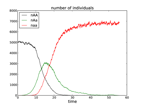
Figure 4.1: Simulation of the three phases of mutant invasion.

In the first phase (between time 0 and $t_{1}$ in Fig. 4.1), the number of mutant individuals of genotype $Aa$ or $aa$ is small, and the resident population with genotype $AA$ stays close to its equilibrium density $\bar{{n}}_{AA}$. Therefore, the dynamics of the mutant individuals with genotypes $Aa$ and $aa$ is close to a bi-type birth and death process with birth rates $f_{Aa}y+2f_{aa}z$ and $0$ and death rates $(D_{Aa}+C_{Aa,AA}\bar{{n}}_{AA})\,y$ and $(D_{aa}+C_{aa,AA}\bar{{n}}_{AA})\,z$ for a state $(y,z)$. If the fitness $S_{Aa;AA}$ is positive (i.e. the branching process is super-critical), the probability that the mutant population with genotype $Aa$ or $aa$ reaches $K\,\varepsilon>0$ at some time $t_{1}$ is close to the probability that the branching process reaches $K\,\varepsilon>0$, which is itself close to its survival probability $\frac{[S_{Aa;AA}]_{+}}{f_{Aa}}$ when $K$ is large.

Assuming the mutant population with genotype $Aa$ or $aa$ reaches $K\,\varepsilon>0$, a second phase starts. When $K\rightarrow+\infty$, the population densities $(\langle\nu_{t}^{\sigma,K},\mathbbm{1}_{\{AA\}}\rangle,\langle\nu_{t}^{\sigma,K},\mathbbm{1}_{\{Aa\}}\rangle,\langle\nu_{t}^{\sigma,K},\mathbbm{1}_{\{aa\}}\rangle)$ are close to the solution of the dynamical system (3.17) with the same initial condition, on any time interval $[0,T]$. The study of this dynamical system (see Appendices B and C) implies that, if the mutation step $u_{a}-u_{A}$ is sufficiently small, then any solution to the dynamical system starting in some neighborhood of $(\bar{n}_{AA},0,0)$ converges to the new equilibrium $(0,0,\bar{n}_{aa})$ as time goes to infinity. Therefore, with high probability the population densities reach the $\varepsilon$-neighborhood of $(0,0,\bar{n}_{aa})$ at some time $t_{2}$. Applying the results in Theorems C.1 and C.2 for the deterministic system to the approximated stochastic process, is justified by observing that the definition of the stopping times $T^{\sigma,K}_{\eta}$ and $T^{\sigma}_{\eta}$ implies that the allelic trait $u_{A}$ stays at all times away from the set $J$.

Finally, in the last phase, we use the same idea as in the first phase: since $(0,0,\bar{n}_{aa})$ is a strongly locally stable equilibrium, we can approximate the densities of the traits $AA$ and $Aa$ by a bi-type sub-critical branching process. Therefore, they reach $0$ in finite time and the process comes back to where we started our argument (a monomorphic population), until the next mutation.

In Champagnat and Méléard (2011) it is proved that the duration of these three phases is of order ${\log K\over\sigma}$. Therefore, under the assumption

$$\log K\ll\frac{\sigma}{K\mu_{K}},$$

the next mutation occurs after these three phases with high probability. Then the time scale Assumption (4.2) allows us to conclude, taking the limits $K$ tending to infinity and then $\varepsilon$ to $0$. Then we repeat the argument using the Markov property.

Note that the convergence cannot hold for the usual Skorohod topology and the space ${\cal M}_{F}$ equipped with the corresponding weak topology. Indeed, it can be checked that the total mass of the limit process is not continuous, which would be in contradiction with the $C$-tightness of the sequence $(\nu^{\sigma,K}_{t/K\mu_{K}},t\geq 0)$, which would hold in case of convergence in law for the Skorohod topology (since the jump amplitudes are equal to ${1\over K}$ and thus tend to $0$ as $K$ tends to infinity).

However, certain functionals of the process converge in a stronger sense. Let us for example consider the average over the population of the phenotypic trait $\phi$. This can be easily extended to more general symmetric functions of the allele.

Theorem 4.7

Assume that $u\to\phi(u,u)$ is strictly monotone. Define

$$T_{\phi,\eta}^{\sigma,K}=\inf\left\{t>0,d\left(\frac{\langle\nu^{\sigma,K}_{t/K\mu_{K}},\phi\rangle}{\langle\nu^{\sigma,K}_{t/K\mu_{K}},1\rangle},J_{\phi}\right)\leq\eta\right\},$$

where $J_{\phi}=\{\phi(u,u);u\in J\}$.

Under the assumptions of Theorem 4.5, the process

$$(R^{\sigma,K}_{t},t\geq 0)=\left(\frac{\langle\nu^{\sigma,K}_{t/K\mu_{K}},\phi\rangle}{\langle\nu^{\sigma,K}_{t/K\mu_{K}},1\rangle}\,\mathbbm{1}_{\{T^{\sigma,K}_{\phi,\eta}\geq t\}},\,t\geq 0\right)$$

converges in law in the sense of the Skorohod $M_{1}$ topology to the process $(\phi(Z^{\sigma}_{t}Z^{\sigma}_{t})\mathbbm{1}_{\{T^{\sigma}_{\phi,\eta}\geq t\}},\\ t\geq 0)$ where $T^{\sigma}_{\phi,\eta}=\inf\left\{t>0,d\left(\phi(Z^{\sigma}_{t},Z^{\sigma}_{t}),J_{\phi}\right)\leq\eta\right\}$.

The Skorohod $M_{1}$ topology is a weaker topology than the usual $J_{1}$ topology, allowing processes with jumps tending to $0$ to converge to processes with jumps (see Skorohod (1956)). For a càd-làg function $x$ on $[0,T]$, the continuity modulus for the $M_{1}$ topology is given by

$$w_{\delta}(x)=\sup_{\stackrel{{\scriptstyle\scriptstyle 0\leq t_{1}\leq t\leq t_{2}\leq T;}}{{0\leq t_{2}-t_{1}\leq\delta}}}d(x(t),[x(t_{1}),x(t_{2})]).$$

Note that if the function $x$ is monotone, then $w_{\delta}(x)=0$.

Proof 9 From the results of Theorem 4.5, it follows easily that finite dimensional distributions of $(R^{\sigma,K}_{t},t\geq 0)$ converge to those of $(\phi(Z^{\sigma}_{t},Z^{\sigma}_{t}),t\geq 0)$. By Skorohod (1956) Theorem 3.2.1, it remains to prove that for all $\eta>0$,

$$\lim_{\delta\to 0}\limsup_{K\to\infty}\mathbb{P}(w_{\delta}(R^{\sigma,K}_{t})>\eta)=0.$$

The rate of mutations of $(R^{\sigma,K}_{t},t\leq T)$ being bounded, the probability that two mutations occur within a time less that $\delta$ is $o(\delta)$. It is therefore enough to study the case where there is at most one mutation on the time interval $[0,\delta]$. As in the proof of Proposition 3.2, with probability tending to $1$ when $K$ tends to infinity, the process $(R^{\sigma,K}_{t},t\geq 0)$ is close to $F_{W_{\phi}}({t/K\mu_{K}})$ where $F_{W_{\phi}}$ is defined by

$$F_{W_{\phi}}(t)=\frac{\langle\varphi_{t}(M_{0})\;,\;W_{\phi}\rangle}{\langle\varphi_{t}(M_{0})\;,\;1\rangle}\;,$$

and

$$W_{\phi}=\left(\begin{array}[]{c}\phi\big{(}u_{A},u_{A}\big{)}\\ \phi\big{(}u_{A},u_{a}\big{)}\\ \phi\big{(}u_{a},u_{a}\big{)}\\ \end{array}\right)\;.$$

Recall that $\varphi_{t}$ is the flow defined by the vector field (see Proposition 3.2). Away from invading mutations, the function $F_{W_{\phi}}$ is constant and the modulus of continuity tends to $0$. Around an invading mutation, it follows from Corollary C.4 that the function $F_{W_{\phi}}$ is monotone. Therefore the same conclusion holds.

$\square$

5 Small mutational steps - the time scale of the canonical equation

We are now interested to study the convergence of the TSS when the mutation amplitude $\sigma$ tends to zero. Without rescaling time, the TSS trivially tends to a constant. In order to get a nontrivial limit, we have to rescale time adequately, namely with ${1\over\sigma^{2}}$, since $S(u_{A};u_{A})=0$.

Theorem 5.1

Assume that the initial values $Z^{\sigma}_{0}$ are uniformly bounded in $L^{2}$ and that they converge to $Z^{0}_{0}$ as $\sigma$ tends to $0$. Then, the sequence of processes $(Z^{\sigma}_{{t/\sigma^{2}}},t\geq 0)$ tends in law in $\mathbb{D}([0,T],\mathbb{R})$ to the deterministic (continuous) solution $(u(t),t\geq 0)$ of the canonical equation

$${d\over dt}u(t)=\,f(u(t),u(t))\,\bar{n}(u(t))\,\int_{\mathbb{R}}h\,[h\,\partial_{1}S(u(t);u(t))]_{+}\,m(u(t),h)dh,$$ (5.1)

where

$$\bar{n}(u)=\frac{f(u,u)-D(u,u)}{C((u,u),(u,u))}.$$

The proof of this theorem is similar to the proof of Theorem 4.1 in Champagnat and Méléard (2011).

In this general form the canonical equation is still of little practical use, although already some qualitative conclusions can be drawn from it. The trait increases whenever the fitness gradient $\partial_{1}S(u;u)$ is positive and decreases when it is negative, i.e., movement is always uphill with respect to the current allelic fitness landscape $S(\cdot;u)$. The equilibria of (5.1) correspond to the allelic evolutionarily singular strategies, except that close to those strategies (5.1) is no longer applicable since in their neighborhood the convergence of the underlying individual-based process to the simple TSS becomes slower and slower. So all we can deduce from the canonical equation (5.1) is that for small mutational steps the trait substitution sequence will move to some close neighborhood of an allelic evolutionarily singular strategy.

Remark 5.2

If we had considered extended TSSes taking values in the powers of the trait space as is done in Metz et al. (1996), the convergence to the canonical equation would similarly have gone awry due to a slowing down of the convergence near evolutionarily singular strategies, and the occurrence of polymorphism close to some of them, with adaptive branching as a particularly salient example; branching can only be investigated with a time scaling different from the one for the canonical equation Metz et al. (1996); Champagnat and Méléard (2011).

To get from the previous observation to some biological conclusion we need to decompose the genotypic fitness function $S$ into its ecological and developmental components

$$\begin{array}[]{rl}S_{Aa,AA}=&\tilde{S}(\phi_{Aa};\phi_{AA})=\tilde{f}(\phi_{Aa})-\tilde{D}(\phi_{Aa})-\tilde{C}(\phi_{Aa},\phi_{AA})\frac{\tilde{f}(\phi_{AA})-\tilde{D}(\phi_{AA})}{\tilde{C}(\phi_{AA},\phi_{AA})},\\ \phi_{Aa}=&\phi(u_{A},u_{a}),\quad\phi_{AA}=\phi(u_{A},u_{A}),\quad\tilde{f}(\phi_{Aa})=f(u_{A},u_{a}),\quad\mathrm{etc.}\end{array}$$ (5.2)

and

$$\partial_{1}S(u;u)=\partial_{1}\tilde{S}(\phi(u;u);\phi(u;u))\partial_{1}\phi(u,u).$$ (5.3)

Hence, the allelic singular strategies are of two different types, ecological, characterized by $\tilde{S}(\phi(u;u);\phi(u;u))=0$, and developmental, characterized by $\partial_{1}\phi(u,u)=0$. On the phenotypic level the latter are perceived as developmental constraints (c.f. Van Dooren (2000)).

To arrive at quantitative conclusions we have to make additional assumptions about the within individual processes. One often used assumption is that the mutation distribution is symmetric. With that assumption (5.1) reduces to

$${d\over dt}u(t)=\,{1\over 2}\,\bar{n}(u(t))\,V_{\mathrm{a}}(u(t))\partial_{1}S(u(t);u(t)),$$ (5.4)

with $V_{\mathrm{a}}$ the allelic mutational variance. (The factor ${1\over 2}$ comes from the fact that the integration is only over a half-line.) This equation can easily be lifted to the phenotypic level as

$${d\over dt}U(t)=\,\bar{n}(U(t))\,V_{\mathrm{p}}(U(t))\partial_{1}\tilde{S}(U(t);U(t)),$$ (5.5)

with $U=\phi(u,u)$ and $V_{\mathrm{p}}$ the phenotypic mutational variance, an equation fully phrased in population level observables. The factor ${1\over 2}$ is canceled by a factor 2 coming from the fact that the fitness $\tilde{S}$ refers to heterozygotes with only one mutant allele, while after a substitution the other allele is also a mutant one. For this equation only the ecological singular strategies remain while developmental constraints appear in the form of $V_{\mathrm{p}}$ becoming zero (c.f. Van Dooren (2000)). (It is also possible to lift (5.1) to the phenotypic level. However, the truncated first and second moments that appear in the resulting expression are no longer well-established statistics that can be measured independent of any knowledge of the surrounding ecology.)

6 Discussion

This paper forms part of a series by a varied collection of authors that aim at putting the tools of adaptive dynamics on a rigorous footing Metz, Nisbet and Geritz (1992); Dieckmann and Law (1996); Metz et al. (1996); Geritz et al. (1998); Champagnat, Ferrière and Méléard (2008); Champagnat (2006); Durinx, Metz and Meszéna (2008); Méléard and Tran (2009); Champagnat and Méléard (2011); Metz (in press); Klebaner et al. (2011); Bovier and Champagnat (in preparation) (see also Diekmann et al. (2005); Barles and Perthame (2007); Carrillo, Cuadrado and Perthame (2007); Desvillettes et al. (2008)). It is the first in the series to treat the individual-based justification of the adaptive dynamics tools in a genetic setting. As such it forms the counterpart of the more heuristic, but also more general Metz (in press). We only consider unstructured Lotka-Volterra type populations and single locus genetics, in line with applied papers such as Kisdi and Geritz (1999); Van Dooren (1999); Proulx and Phillips (2006); Peischl and Bürger (2008). For such models we proved the convergence (for large population sizes and suitably small mutation probabilities) of the individual-based stochastic process to the TSS of adaptive dynamics, and the subsequent convergence (for small mutational steps) of the TSS to the canonical equation. Not wholly unexpectedly, the results are in agreement with the assumed framework of the more applied work. Yet, to arrive at a rigorous proof new developments were needed, like the derivation of a rigorous estimate for the probability of invasion in a dynamic diploid population (Appendix D), a rigorous, geometric singular perturbation theory based, invasion implies substitution theorem (appendix C), and the use of the Skorohod $M_{1}$ topology to arrive at a functional convergence result for the TSS (Section 4).

Below we list the remaining biological limitations of the present results and the corresponding required further developments.

The first limitation is the assumption of an unstructured population. For a a fair number of real populations the assumption of random deaths appears to match the observations, but no organisms reproduce in a Poisson process starting at birth. Moreover, in nature a good amount of population regulation occurs through processes affecting the birth rate, as when a scarcity of resources translates in a delay of maturing to the reproductive condition. Durinx, Metz and Meszéna (2008) heuristically treats very general life histories (although only for a finite number of birth states, a finite number of variables channeling the interaction between individuals, and a deterministic population dynamics converging to a unique equilibrium) based on the population dynamical modeling framework of Diekmann et al. (1998, 2001); Diekmann, Gyllenberg and Metz (2003). However, it only considers the convergence to the canonical equation, starting from the TSS, conjectured to be derivable from the population dynamical model, with the goal of relating its coefficient functions to observationally accessible statistics of individual behavior. In fact, even the convergence to a deterministic population model, as in Theorem 3.1, does not easily fit in the scheme of Fournier and Méléard (2004) in the (biologically common) cases where the movement of individuals through their state spaces depends directly or indirectly on the population size and composition. (The special case where this movement decomposes in a product of a population- and a state-dependent term is covered in Tran (2006, 2008); Ferrière and Tran (2009)).

A further limitation is that we assumed the trait to be governed by only a single locus (in keeping with a well-established tradition starting with Kimura (1965)). The more locus case still has to be worked out. The superficially more easy case with infinitely many loci, so that no mutant ever occurs on the same locus, is considered from a heuristic perspective in Metz (in press); Metz and de Kovel (in preparation). However, the problem of rigorously setting up the underlying individual-based model as a limit for models with an ever increasing number of loci still needs to be tackled.

The final extension to be considered is to higher dimensional geno- and phenotypic trait spaces. We conclude with a heuristic discussion of the form such an extension will take. On the genotypic level the canonical equation will take essentially the same form as (5.1) and (5.4), with scalar $u$, $h$ and $\partial_{1}S$ replaced by vectors, and the mutational variance by a covariance matrix, just as this is written in Dieckmann and Law (1996); Champagnat, Ferrière and Méléard (2008); Durinx, Metz and Meszéna (2008); Champagnat and Méléard (2011) for the clonal and Metz (in press); Metz and de Kovel (in preparation) for the Mendelian case. However, there is one remaining snag, which is the reason why we opted for treating only the one-dimensional case. In the directions orthogonal to the selection gradient the fitness landscape around the resident strategy has the same shape as at an evolutionarily singular strategy. In the one-dimensional case we opted for just removing the neighborhoods of the singular strategies. If we were to apply the same strategy for the higher dimensional case we would have to remove all residents. The way out is by observing that the directions where something awry may occur are but a very small minority among all possible directions in which mutations may occur. Heuristic calculations suggest that the trouble only occurs in a narrow double horn with a boundary that at the resident strategy is tangent to the linear manifold orthogonal to the selection gradient, so that when the mutational step size $\sigma$ goes to zero, the probability of a mutant ending up in that horn decreases as some higher power of $\sigma$. Moreover, in the directions orthogonal to the fitness gradient the fitness is a quadratic function, making the probability of invasion scale not linearly but quadratically with the size of any mutational steps in those directions. The main problem with such mutants is that some of them may on the population dynamical time scale keep coexisting with the resident. Further heuristic calculations then suggest that for such a resident pair the probability of invasion of a subsequent mutant more in the direction of the fitness gradient is to the lowest order of approximation - in the distance between the two residents - equal to the probability of invasion in a monomorphic population of the average type, and that such a mutant ousts both residents. Therefore the general (i.e., more type) TSS is close to a simple TSS in which those untoward mutants are just removed from the consideration, the smaller the mutational step the closer. We put rigorously underpinning this scenario forward as the last of our list of challenges.

Acknowledgements: This work benefitted from the support from the "Chair Modélisation Mathématique et Biodiversité of Veolia Environnement-Ecole Polytechnique-Museum National d’Histoire Naturelle-Fondation X" and from the ANR MANEGE.

Appendices

Appendix A A few words about competition kernels

In the ecological literature the models described in Section 2 are known as Lotka-Volterra competition models Lotka (1925); Volterra (1931). The early LV models were all deterministic, phrased as ODEs corresponding to large population limits such as considered in the Section 3, without mutations. The determinism together with the assumption of clonal reproduction obviated the need to separately model birth and deaths: competition was represented as its overall effect on the population growth rate. The later stochastic models, e.g. Dieckmann and Law (1996); Metz et al. (1996), usually put the effect of competition only in the death rate, as otherwise the chosen linear form of the interaction might lead to negative birth rates.

The simplest case is when $C=0$. This is the case customarily put forward in population genetics textbooks as starting point for the derivation of their deterministic models for gene frequency change by selection, but for the fact that population geneticists usually work in discrete time. The unnatural consequence that the population either will die out or will keep growing indefinitely is made invisible by transforming to relative frequencies. The more realistic case of non-selective competition, $C((u_{1},u_{2});(v_{1},v_{2}))=\overset{\lower 5.0pt\hbox{$\smash{\scriptscriptstyle\frown}$}}{C}(v_{1},v_{2})$, leads to the same population genetical equations. The selective pressures on the gene frequencies then do not change with the population size or composition as they are caused only by differences in the fixed mortalities and fertilities.

Where in population genetics the early selection models assumed indefinitely growing populations, the early stochastic models, in continuous time the Moran-type models, assumed constant population sizes. Although later variable population sizes were introduced, it was just assumed that these sizes fluctuated between positive lower and upper bounds Karlin (1968); Donnelly and Weber (1985). Stochastic models with the population regulation represented in accordance with ecological tradition are relative newcomers (e.g. Metz and Redig (in preparation)).

The case where the additional death rate incurred by an individual from its competitive interaction depends only on the genotype of the focal individual and not on that of its competitors is known in the ecological literature as purely density dependent selection Roughgarden (1971, 1976, 1979) , and in the mathematical literature as logistic population regulation. This logistic case can be generalized to $C((u_{1},u_{2});(v_{1},v_{2}))=\overset{\lower 5.0pt\hbox{$\smash{\scriptscriptstyle\smile}$}}{C}(u_{1},u_{2})\overset{\lower 5.0pt\hbox{$\smash{\scriptscriptstyle\frown}$}}{C}(v_{1},v_{2})$, when it is not the total density but e.g. the total biomass that determines the felt competitive effect and different genotypes have different biomasses. A further generalization is that population growth is regulated by a finite number of variables, think for example of the combination of space and nitrogen depletion:

$$C((u_{1},u_{2});(v_{1},v_{2}))=\sum_{i=1}^{k}\overset{\lower 5.0pt\hbox{$\smash{\scriptscriptstyle\smile}$}}{C}_{i}(u_{1},u_{2})\overset{\lower 5.0pt\hbox{$\smash{\scriptscriptstyle\frown}$}}{C}_{i}(v_{1},v_{2}).$$

The vector $(\overset{\lower 5.0pt\hbox{$\smash{\scriptscriptstyle\frown}$}}{C}_{1},\dots,\overset{\lower 5.0pt\hbox{$\smash{\scriptscriptstyle\frown}$}}{C}_{k})^{\mathrm{T}}$ is known as the impact of the individuals on their environment, and the vector $(\overset{\lower 5.0pt\hbox{$\smash{\scriptscriptstyle\smile}$}}{C}_{1},\dots,\overset{\lower 5.0pt\hbox{$\smash{\scriptscriptstyle\smile}$}}{C}_{k})$ as their sensitivity a Meszéna et al. (2006). The latter generalization is evolutionarily richer in that it can allow diversification, which is excluded by the earlier considered kernels. In Durinx, Metz and Meszéna (2008) it is shown heuristically that close to an evolutionarily singular strategy any clonal model evolutionarily behaves like a Lotka-Volterra competition model of the above type with $k$ equal to one plus the dimension of the trait space.

The above considerations all come from either ecology or population genetics, and originally were phrased for a fixed finite number of types, clonal ones in the ecological and Mendelian ones in the population genetics literature. The first model characterizing these types in terms of traits was formulated by Robert MacArthur and Richard Levins MacArthur and Levins (1964), see also MacArthur (1970). This model was later used to great effect by a large number of authors (e.g. Levins (1968); MacArthur and Levins (1967); May (1973, 1974); Roughgarden (1976); Christiansen and Fenchel (1977); Roughgarden (1979); Slatkin (1980), but see also Roughgarden (1989)) to study species packing population dynamically as well as evolutionarily. The first genetic model of this type was studied by Freddy Bugge Christiansen and Volker Loeschcke Christiansen and Loeschcke (1980); Loeschcke and Christiansen (1984); Christiansen and Loeschcke (1987) , who considered the possibilities for the coexistence of finite numbers of genotypes. Explicit trait-based LV-style birth and death process models with mutation only appeared on the scene with the birth of adaptive dynamics Dieckmann and Law (1996); Metz et al. (1996).

The most common assumption in trait-based LV competition models MacArthur and Levins (1964); MacArthur (1970, 1972); Roughgarden (1979) is that

$$C((u_{1},u_{2});(v_{1},v_{2}))=C((u_{1},u_{2});(u_{1},u_{2})){\int Q(u_{1},u_{2})q((u_{1},u_{2});z)Q(v_{1},v_{2})q(v_{1},v_{2};z)\mathrm{d}z\over\int Q^{2}(u_{1},u_{2})q^{2}((u_{1},u_{2});z)\mathrm{d}z}.$$

Here $z\in\mathbb{R}$ is customarily interpreted as a trait of a fine-grained self-renewing resource with a fast logistic dynamics that is supposed to be non-evolving. That is, it is assumed that a resource unit comprises close to infinitely many very small particles, so that the resource dynamics can be treated as deterministic and that the turnover of the resource is very fast so that it effectively tracks its deterministic equilibrium as set by the current consumer population. Functions of $(u_{1},u_{2})$ depend again on this argument through $\phi$. $Q$ is the average rate constant for the encounter and absorption of resource particles by our consumer individuals, expressed in resource units, while $q$ tells how this use is spread over the resource axis.

The most commonly used parametric form is

$$f(u_{1},u_{2})-D(u_{1},u_{2})=:r(u_{1},u_{2})=\bar{r},$$

$${{r(u_{1},u_{2})}\over{C(u_{1},u_{2});(u_{1},u_{2}))}}=:k(u_{1},u_{2})=\exp\left(-\frac{\left(\phi(u_{1},u_{2})-\phi_{0}\right)^{2}}{2\sigma_{k}^{2}}\right),$$

$$Q(u_{1},u_{2})q((u_{1},u_{2});z)=\exp\left(-\frac{\left(z-\phi(u_{1},u_{2})\right)^{2}}{\sigma_{a}^{2}}\right),$$

leading to

$$C((u_{1},u_{2});(v_{1},v_{2}))=\bar{r}\exp\left(-\frac{\left(\phi(u_{1},u_{2})-\phi(v_{1},v_{2})\right)^{2}}{2\sigma_{a}^{2}}+\frac{\left(\phi(u_{1},u_{2})-\phi_{0}\right)^{2}}{2\sigma_{k}^{2}}\right)$$

Deterministic models based on this kernel have all sorts of nice mathematical properties, but Adaptive Dynamically they are a bit degenerate in that when $\sigma_{a}<\sigma_{k}$ the final stop for trait substitution sequences that result from the long term large population and rare mutations limit, as treated in Section 4, is a Gaussian distribution over trait space (c.f. Roughgarden (1979)) whereas for almost any slightly different model the final stop has finite support Gyllenberg and Meszéna (2005); Leimar, Doebeli and Dieckmann (2008). For this reason adaptive dynamics researchers started to use slightly modified expressions for $k$ or $C$. (When $K$ is still finite, the number of branches visible in simulations also stays finite, due to the early abortion of incipient ones, with the number of recognizable branches becoming larger with increasing $K$ and $\sigma_{k}/\sigma_{a}$ Claessen et al. (2007, 2008).) Exploring the consequences of all sorts of different competition kernels by now has become a little growth industry; a good sample may be found in Doebeli (2011).

Remark A.1

The description of the mechanism underlying the competition kernel given above was a bit brash, in keeping with biological tradition. Starting from an underlying fast logistic resource dynamics actually gives

$$f(u_{1},u_{2})=y(\phi(u_{1},u_{2}))\left(\int{v(\phi(u_{1},u_{2}),z)w(z)k_{\mathrm{R}}(z)\mathrm{d}z-d_{1}(\phi(u_{1},u_{2}))}\right),$$

$$D(u_{1},u_{2})=d_{2}(\phi(u_{1},u_{2}))$$

$$C((u_{1},u_{2});(v_{1},v_{2}))=y(x)\int{v(\phi(u_{1},u_{2});z)\frac{w(z)k_{\mathrm{R}}(z)}{r_{\mathrm{R}}(z)}v(\phi(v_{1},v_{2});z)\mathrm{d}z}$$

and hence

$$Q(u_{1},u_{2})q((u_{1},u_{2});z)=Vv(\phi(u_{1},u_{2});z)\left(\frac{w(z)k_{\mathrm{R}}(z)}{r_{\mathrm{R}}(z)}\right)^{{1}/{2}}$$

with $y$ the yield, i.e., $y^{-1}$ is the resource mass needed to make one consumer, $w$ the mass of a resource unit, $v$ the rate constant of consumers encountering and eating resource units, $d_{1}$ the rate constant of consumer mass loss due to basal metabolism, and $d_{2}$ the consumer mortality rate, $r_{\mathrm{R}}$ the low density reproductive rate of the resource, and $k_{\mathrm{R}}$ its carrying capacity. $V$ is some unknown proportionality constant. (In the above terms the time scale separation results from both $r_{\mathrm{R}}$ and $v$ being very large and $y$ very small with the product of $y$ and $v$ being $\mathrm{O}(1)$.) Apparently the interpretation of $Q$ and $q$ is more complicated than the standardly attributed one based on the assumption of constant $wk_{\mathrm{R}}/r_{\mathrm{R}}$.

Although time-honoured, the above described mechanistic underpinning is not without flaws, as explicitly laid out by Chesson (1990). In the derivation it is assumed that, but for the indirect coupling through the consumers, the dynamics of different resources are independent. Even very similar resource populations do not compete. However, this is only possible if their ecological properties depend everywhere discontinuously on the trait $z$, since the assumed logistic nature of the resource dynamics means that there is non-negligible competition between equal resource particles. The alternative assumption alluded to by MacArthur MacArthur (1972) that the intrinsic resource dynamics is of a chemostat type (as can be approximately the case for seeds from perennial plants) also is problematical: Under the reasonable assumption that the resource mass removed by a consumer population equals the mass this population acquires, the detrimental effect from competition becomes non-linear in the competitor densities, instead of being simply representable by a competition kernel.

Appendix B Properties of the vector field (3.21.)

B.1 Neutral case.

We first consider the case of neutrality between the $A$ and $a$ alleles, namely $f_{a_{1}a_{2}}=f$, $D_{a_{1}a_{2}}=D^{0}$ and $C_{a_{1}a_{2}\,,\,b_{1}b_{2}}=D^{1}$ for $a_{1}a_{2},b_{1}\,b_{2}=AA,Aa,aa$. We have in this case with $n=x+y+z$

$$p=\frac{x+y/2}{n}$$

which is the proportion of allele $A$. We get for the vector field

$$X_{0}=\left(\begin{array}[]{c}f(x+y/2)p-(D^{0}+D^{1}n)x\\ f(x+y/2)(1-p)+f(z+y/2)p-(D^{0}+D^{1}n)y\\ f(z+y/2)(1-p)-(D^{0}+D^{1}n)z\\ \end{array}\right)$$

Theorem B.1

The vector field $X_{0}$ has a line of fixed points given by

$$\Gamma_{0}(v)=\begin{pmatrix}{\frac{\displaystyle v^{2}-2\,{n_{0}}\,v+{n_{0}}^{2}}{\displaystyle 4\,{n_{0}}}}\cr-{\frac{\displaystyle v^{2}-{n_{0}}^{2}}{\displaystyle 2\,{n_{0}}}}\cr\frac{\displaystyle{v^{2}+2\,{n_{0}}\,v+{n_{0}}^{2}}}{\displaystyle 4\,{n_{0}}}\cr\end{pmatrix}\;,$$

with $n_{0}=(f-D^{0})/D^{1}$. That is, we have for any $v$, $X_{0}(\Gamma_{0}(v))=0$. The parametrization with $v$ is chosen such that the differential of the vector field $X_{0}$ at each point of the curve $\Gamma_{0}$, $DX_{0}(\Gamma_{0}(v))$, has the three eigenvectors

$$e_{1}(v)=\Gamma_{0}(v))=\begin{pmatrix}\frac{\displaystyle v^{2}-2\,{n_{0}}\,v+{n_{0}}^{2}}{\displaystyle 4\,{n_{0}}}\cr-\frac{\displaystyle v^{2}-{n_{0}}^{2}}{\displaystyle 2\,{n_{0}}}\cr\frac{\displaystyle v^{2}+2\,{n_{0}}\,v+{{n_{0}}^{2}}}{\displaystyle 4\,{n_{0}}}\cr\end{pmatrix}\;,$$

$$e_{2}(v)=\frac{\displaystyle d\Gamma_{0}(v)}{\displaystyle dv}=\begin{pmatrix}\frac{\displaystyle v-n_{0}}{\displaystyle 2\,n_{0}}\cr-\frac{\displaystyle v}{\displaystyle n_{0}}\cr\frac{\displaystyle v+n_{0}}{\displaystyle 2\,n_{0}}\cr\end{pmatrix}\;,$$

$$e_{3}(v)=\frac{\displaystyle d^{2}\Gamma_{0}}{\displaystyle dv^{2}}=\frac{1}{2n_{0}}\begin{pmatrix}1\\ -2\\ 1\\ \end{pmatrix}$$

with respective eigenvalues $D^{0}-f<0$, $0$, and $-f<0$. The corresponding eigenvectors of the transposed matrix $DX_{0}(\Gamma_{0}(v))^{t}$, to be denoted by by $\beta_{1}(v)$, $\beta_{2}(v)$ and $\beta_{3}(v)$ can be normalized such that for any $i,j,\in\{1,2,3\}$ and any $v$

$$\langle\beta_{i}(v)\,,\,e_{j}(v)\rangle=\delta_{i,j}\;.$$

Proof 9 This is easily seen by using the standard variables: total population density, $n=x+y+z$, relative frequency of the $A$ allele, $p=(x+y/2)/n$, and excess heterozygosity realtive to the Hardy-Weinberg proportion, $h=y/n-2p(1-p)$.

In these new coordinates, the vector field $X_{0}$ becomes the vector field $Y_{0}$ given by

$$Y_{0}(n,p,h)=\left(\begin{array}[]{c}f-(D^{0}+D^{1}\,n)\,n\\ 0\\ -f\,h\\ \end{array}\right)\;.$$

This vector field obviously vanishes on the line $n=n_{0},\;h=0$. One gets immediately the results by taking $v=n_{0}\,(1-2\,p)$. The spectral results follow by standard computations. $\square$

B.2 Small perturbations.

We now assume that mutations are small. We denote by $\zeta$ the variation of the allelic trait $\zeta=u_{a}-u_{A}$. The vector field depends on $\zeta$ and will be denoted by $X(\zeta,M)$. We assume regularity in $\zeta$ and $M$, and observe that $X(0,M)=X_{0}(M)$.

In practice we will apply our results to the vector field (3.21) which has a particular algebraic form. It is however convenient to derive the perturbation results in full generality. We will come back to the particular case of (3.21) in section C.

From now on, we will assume that the vector field $X(\zeta,\,\cdot\,)$ satisfies the following properties for any $x$, any $z$ and any $\zeta$

$$X_{x}\big{(}\zeta,(0,0,z)\big{)}=X_{y}\big{(}\zeta,(0,0,z)\big{)}=0\;,$$

and

$$X_{z}\big{(}\zeta,(x,0,0)\big{)}=X_{y}\big{(}\zeta,(x,0,0)\big{)}=0\;.$$ (B.1)

This comes from the fact that pure homozygotic populations stay pure homozygotic forever.

Our goal in this section is to understand the time asymptotic of the flow associated to the vector field $X(\zeta,M)$.

Since the curve $\Gamma_{0}$ is transversally hyperbolic (even transversally contracting, see Proposition B.1) for the vector field $X_{0}$, we can apply Theorem 4.1 in Hirsh, Pugh and Shub, M. (1977) to conclude that for $\zeta$ small enough, there is an attracting curve $\Gamma_{\zeta}$ invariant by $X$. Moreover, $\Gamma_{\zeta}$ is regular and converges to $\Gamma_{0}$ when $\zeta$ tends to zero. In other words, there is a small enough tubular neighborhood $\mathscr{V}$ of $\Gamma_{0}$ such that for any $|\zeta|$ small enough, $\Gamma_{\zeta}$ is contained in $\mathscr{V}$ and attracts all the orbits with initial conditions in $\mathscr{V}$. (For earlier, weaker results in this direction for general differential and difference equation population dynamical models without genetics see (Geritz et al., 2002; Dercole and Rinaldi, 2008, Appendix B).)

Applying Theorem 4.1 in Hirsh, Pugh and Shub, M. (1977) requires that the curve $\Gamma_{0}$ is a compact manifold without boundary, but this is not the case here. However one can perform some standard surgery to put our problem in this form in a neighborhood of the part of $\Gamma_{0}$ which lies in the positive quadrant which is the only part of phase space that matters for us.

B.2.1 Location of the zeros of the perturbed vector field.

Since the curve $\Gamma_{\zeta}$ is invariant and (locally) attracting for the flow associated to the vector field $X(\zeta,M)$, where $M$ stands for the vector $x,y,z)$ it is enough to study the flow on this curve. In particular, since $\Gamma_{\zeta}$ is a curve, if the vector field does not vanish on $\Gamma_{\zeta}$ except at the intersections with the lines $x=y=0$ and $y=z=0$ (the fixed points $aa$ and $AA$ respectively see Theorem 3.3), we know that the orbit of any initial condition on $\Gamma_{\zeta}$ (between $AA$ and $aa$) will converge either to $AA$ or to $aa$.

We now look for the fixed points on $\Gamma_{\zeta}$ of the flow associated to the vector field $X(\zeta,M)$ which are the points where the vector field vanishes. Since $\Gamma_{\zeta}$ is attracting, it is equivalent (and more convenient) to look for the fixed points in $\mathscr{V}$.

It is convenient to use for this study local frames in the tubular neighborhood $\mathscr{V}$ of $\Gamma_{0}$. There are many possibilities for defining such frames, we found that a convenient one is to represent a point $M$ by the parametrisation

$$M(v,r,s)=\Gamma_{0}(v)+re_{1}(v)+se_{3}(v)=(1+r)\Gamma_{0}(v)+s\frac{d^{2}\Gamma_{0}(v)}{dv^{2}}\;.$$

with $v\in[-n_{0}-\delta,n_{0}+\delta]$, $r\in[-\delta,\delta]$, $s\in[-\delta,\delta]$ with $\delta>0$ to be chosen small enough later on. We observe that $M(v,0,0)=\Gamma_{0}(v)$.

The Jacobian of the transformation $(v,r,s)\mapsto(x,y,z)=M(v,r,s)$ is equal to $-(1+r)/2$ and therefore does not vanish if $0<\delta<1$. It is easy to verify that if $\delta>0$ is small enough, the map $(v,r,s)\mapsto M(v,r,s)$ is a diffeomorphism of $[-n_{0}-\delta,n_{0}+\delta]\times[-\delta,\delta]^{2}$ to a close neighborhood of $\mathscr{V}$ (provided this tubular neighborhood is small enough). In particular, once $\delta>0$ is chosen, for any $\zeta>0$ small enough, $\mathscr{V}$ contains the intersection of $\Gamma_{\zeta}$ with the first quadrant (by continuity of $\Gamma_{\zeta}$ in $\zeta$).

In order to find the zeros of the vector field $X(\zeta,M)$, we will use convenient linear combinations of its components which reflect the fact that the flow is transversally hyperbolic. We will first equate to zero two linear combinations of the components, and by the implicit function theorem this will lead to a curve containing all possible zeros. We will then look at the points on this curve where the third (independent) linear combination of the components vanishes.

Proposition B.2

For any $\delta>0$ small enough, there is a number $\zeta_{0}=\zeta_{0}(\delta)$ such that for any $\zeta\in[-\zeta_{0},\zeta_{0}]$ there is a smooth curve $\mathscr{Z}_{\zeta}=(r_{\zeta}(v),s_{\zeta}(v))\subset{\mathbb{R}}^{2}$, depending smoothly on $\zeta$, and converging to $0$ when $\zeta$ tends to zero such that for any $v\in[-n_{0}-\delta,n_{0}+\delta]$ we have

$$\langle\beta_{1}(v)\,,\,X\big{(}\zeta,M(v,r_{\zeta}(v),s_{\zeta}(v))\big{)}\rangle=\langle\beta_{3}(v)\,,\,X\big{(}\zeta,M(v,r_{\zeta}(v),s_{\zeta}(v))\big{)}\rangle=0\;.$$

Moreover, if a point $(v,r,s)$ with $v\in[-n_{0}-\delta,n_{0}+\delta]$, $r$ and $s$ small enough is such that

$$\langle\beta_{1}(v)\,,\,X\big{(}\zeta,M(v,r,s)\big{)}\rangle=\langle\beta_{3}(v)\,,\,X\big{(}\zeta,M(v,r,s)\big{)}\rangle=0$$

then $(r,s)=(r_{\zeta}(v),s_{\zeta}(v))$.

Proof 9 Consider the map $F$ from ${\mathbb{R}}^{2}\times{\mathbb{R}}^{2}$ to ${\mathbb{R}}^{2}$ given by

$$F\big{(}(\zeta,v),(r,s)\big{)}=\big{(}\langle\beta_{1}(v)\,,\,X\big{(}\zeta,M(v,r,s)\big{)}\rangle,\langle\beta_{3}(v)\,,\,X\big{(}\zeta,M(v,r,s)\big{)}\rangle\big{)}\;.$$

For any $v_{0}\in[-n_{0}-\delta,n_{0}+\delta]$, and $|\zeta|$ small enough, the differential of $F$ in $(r,s)$ at $(0,v_{0},0,0)$ is invertible. This follows by continuity from the same result in $\zeta=0$ where the determinant of the differential is $f(f-D^{0})$. Therefore, by the implicit function theorem (see for example Dieudonné (1969)), for any $v_{0}\in[-n_{0}-\delta,n_{0}+\delta]$, there is an open neighborhood $U_{v_{0}}$ of $(v_{0},0)$ in ${\mathbb{R}}^{2}$ and two regular functions functions on $U_{v_{0}}$, $r^{v_{0}}$ and $s^{v_{0}}$ such that for any $(\zeta,v)\in U_{v_{0}}$ we have

$$F\big{(}(\zeta,v),(r^{v_{0}}(\zeta,v),s^{v_{0}}(\zeta,v))\big{)}=0\;.$$

Since the set $[-n_{0}-\delta,n_{0}+\delta]\times\{0\}$ is compact in ${\mathbb{R}}^{2}$, we can find a finite sequence $v_{1},\ldots,v_{m}$ such that the finite sequence of sets $(U_{v_{j}})$ is a finite open cover of $[-n_{0}-\delta,n_{0}+\delta]\times\{0\}$. We now define the functions $r$ and $s$ in the tubular neighborhood $\cup_{j}U_{v_{j}}$ of $[-n_{0}-\delta,n_{0}+\delta]\times\{0\}$ by

$$r(\zeta,v)=r^{v_{j}}(\zeta,v)\;,\quad s(\zeta,v)=s^{v_{j}}(\zeta,v)\;,\quad\mathrm{for}(\zeta,v)\in U_{v_{j}}\;.$$

This definition is consistent since if $(\zeta,v)\in U_{v_{j}}\cap U_{v_{\ell}}$ with $\ell\neq j$ we have $r^{v_{j}}(\zeta,v)=r^{v_{\ell}}(\zeta,v)$ and $s^{v_{j}}(\zeta,v)=s^{v_{\ell}}(\zeta,v)$ by the uniqueness of the solution in the implicit function theorem. The last assertion of the proposition follows also from the uniqueness of the solution in the implicit function theorem. $\square$

It follows immediately from the above result that the vector field $X(\zeta,\,\cdot\,)$ vanishes in a small enough neighborhood of $\Gamma_{0}$ if and only if

$$\langle\beta_{2}(v)\,,\,X\big{(}\zeta,M(v,r_{\zeta}(v),s_{\zeta}(v))\big{)}\rangle=0\;,$$

which at a given $\zeta$ is an equation for $v$.

We analyze a neighborhood of the point $\zeta=0$. We first observe that

$$\langle\beta_{2}(v)\,,\,X\big{(}0,M(v,r_{0}(v),s_{0}(v))\big{)}\rangle=\langle\beta_{2}(v)\,,\,X\big{(}0,M(v,0,0)\big{)}\rangle$$

$$=\langle\beta_{2}(v)\,,\,X\big{(}0,\Gamma_{0}(v))\big{)}\rangle=0\;.$$

Therefore by the Malgrange preparation Theorem Golubitsky and Guillemin (1973) (the Weierstrass preparation Theorem in the analytic setting), we can write

$$\langle\beta_{2}(v)\,,\,X\big{(}\zeta,M(v,r_{\zeta}(v),s_{\zeta}(v))\big{)}\rangle=\zeta^{2}h(\zeta,v)+\zeta g(v)\;.$$ (B.2)

Lemma B.3

The function $g$ in (B.2) is given by

$$g(v)=\langle\beta_{2}(v)\,,\partial_{\zeta}X(0,\Gamma_{0}(v))\rangle\;.$$

Proof 9 We have

$$g(v)=\bigg{\langle}\beta_{2}(v)\,,\,\big{(}\partial_{\zeta}X\big{(}\zeta,M(v,r_{\zeta}(v),s_{\zeta}(v))\big{)}_{\big{|}\zeta=0}\bigg{\rangle}$$

$$=\langle\beta_{2}(v)\,,\,\partial_{\zeta}X\big{(}0,\Gamma_{0}(v)\big{)}\rangle+\bigg{\langle}\beta_{2}(v)\,,\,DX(0,\Gamma_{0}(v))\;\partial_{r}M(v,0,0)\;\partial_{\zeta}r_{\zeta}(v))_{\big{|}\zeta=0}\bigg{\rangle}$$

$$+\bigg{\langle}\beta_{2}(v)\,,\,DX(0,\Gamma_{0}(v))\;\partial_{s}M(v,0,0)\;\partial_{\zeta}s_{\zeta}(v))_{\big{|}\zeta=0}\bigg{\rangle}$$

$$=\langle\beta_{2}(v)\,,\,\partial_{\zeta}X\big{(}0,\Gamma_{0}(v)\big{)}+\bigg{\langle}\beta_{2}(v)\,,\,DX(0,\Gamma_{0}(v))\;e_{1}(v)\;\partial_{\zeta}r_{\zeta}(v))_{\big{|}\zeta=0}\bigg{\rangle}$$

$$+\bigg{\langle}\beta_{2}(v)\,,\,DX(0,\Gamma_{0}(v))\;e_{3}(v)\;\partial_{\zeta}s_{\zeta}(v))_{\big{|}\zeta=0}\bigg{\rangle}\;.$$

The lemma follows at once from Proposition B.1. $\square$

The following result gives conditions for the perturbed vector field to have only two fixed points near $\Gamma_{0}$.

Theorem B.4

Assume the function

$$g(v)=\langle\beta_{2}(v)\,,\partial_{\zeta}X(0,\Gamma_{0}(v))\rangle\;.$$

satisfies $dg/dv(\pm n_{0})\neq 0$ and does not vanish in $(-n_{0},n_{0})$. Then for $|\zeta|$ small enough (but non zero), the vector field $X$ has only two zeros in a tubular neighborhood of $\Gamma_{0}$. These zeros are $(n_{AA}(\zeta),0,0))$ and $(0,0,n_{aa}(\zeta))$ with $n_{AA}(\zeta)$ and $n_{aa}(\zeta)$ regular near $\zeta=0$ and $n_{AA}(0)=n_{aa}(0)=n_{0}$.

As we will see in the proof $g(\pm n_{0})=0$ and the condition $dg/dv(\pm n_{0})\neq 0$ ensures that these zeros are isolated.

Proof 9 We observe that

$$X\big{(}\zeta,\Gamma_{0}(-n_{0})\big{)}=X\big{(}\zeta,n_{0},0,0)\big{)}\;,$$

hence

$$\partial_{\zeta}X_{y}\big{(}\zeta,\Gamma_{0}(-n_{0})\big{)}=\partial_{\zeta}X_{z}\big{(}\zeta,\Gamma_{0}(-n_{0})\big{)}=0\;.$$

On the other hand, by a direct computation one gets

$$\beta_{2}(-n_{0})=\left(\begin{array}[]{c}0\\ 1\\ 2\end{array}\right)$$

and we get $g(-n_{0})=0$ . Similarly one has $g(n_{0})=0$.

Since the functions $g$ and $h$ in (B.2) are regular, for $|\zeta|$ small, it follows that the function $v\to\langle\beta_{2}(v)\,,X\big{(}\zeta,M(v,r_{\zeta}(v),s_{\zeta}(v))\big{)}$ can vanish only in neighborhoods of points where $g$ vanishes. We conclude that if $g$ does not vanish on the open interval $]-n_{0},n_{0}[$, and

$$\frac{dg}{dv}(\pm n_{0})\neq 0\;,$$

there is a number $\delta^{\prime}>0$ such that for $|\zeta|$ small enough non zero, the function $v\to\langle\beta_{2}(v)\,,X\big{(}\zeta,M(v,r_{\zeta}(v),s_{\zeta}(v))\big{)}$ has at most two zeros in the interval $[-n_{0}-\delta^{\prime},n_{0}+\delta^{\prime}]$. Such zeros must be simple and near $\pm n_{0}$. By Theorem 3.3 we conclude that these two zeros exist and are the two fixed points $aa$ and $AA$ respectively. $\square$

Appendix C Applications to the process of mutant substitution

Recall that in our setting, the resident population is monomorphic with genotype $(u_{A},u_{A})$. The mutant allelic trait $u_{a}$ is given by

$$u_{a}=u_{A}+\zeta,$$

where $\zeta$ has been chosen according to the distribution $m_{\sigma}(u_{A},h)dh$ and therefore $|\zeta|\leq\sigma$.

C.1 The stable manifold of the AA fixed point.

As we have seen before in Theorem 3.3 the stability of the fixed point $AA$ can be decided by looking at the fitness of the mutant. We will need later on a property of the stable manifold in the case where this fixed point is unstable.

Theorem C.1

For $|\zeta|$ small enough, if $S_{Aa,AA}(\zeta)>0$, the local stable manifold of the unstable fixed point $AA$ intersects the closed positive quadrant only along the line $y=z=0$. The local unstable manifold is contained in the curve $\Gamma_{\zeta}$.

Proof 9 Hyperbolicity follows from Theorem 3.3, and we can apply Theorem 5.1 in Hirsh, Pugh and Shub, M. (1977). From Theorem 3.3, one finds that the Jacobian matrix $DX_{AA}$ has three eigenvectors

$$E_{1}(\zeta)=e_{1}(-n_{0})+\mathcal{O}(\zeta)\;,\quad E_{2}(\zeta)=e_{2}(-n_{0})+\mathcal{O}(\zeta)\;,\quad E_{3}(\zeta)=e_{3}+\mathcal{O}(\zeta)\;,\quad\;,$$

with respective eigenvalues $D^{0}-f+\mathcal{O}(\zeta)$, $\mathcal{O}(\zeta)$, $-f+\mathcal{O}(\zeta)$.

It follows from Theorem 5.1 in Hirsh, Pugh and Shub, M. (1977) that the local stable manifold $W^{s,\,loc}_{AA}$ of $AA$ is a piece of regular manifold tangent in $AA$ to the two dimensional affine stable subspace $E^{s}_{AA}(\zeta$ with origin in $AA$, and spanned by the vectors $E_{1}(\zeta)$ and $E_{3}(\zeta)$.

The $x$ axis ($y=z=0$) is invariant by the vector field and is contained in the stable manifold. The first result follows from the fact that $E^{s}_{AA}(\zeta)$ intersects the closed positive quadrant only along the line $y=z=0$.

Since the local (one dimensional) unstable manifold $W^{u,\,loc}_{AA}(\zeta)$ of $AA$ is tangent to the linear unstable direction in $E_{2}(\zeta)$ in $AA$, it is enough to show that this direction points inside the quadrant. This follows immediately from the expression of $E_{2}(\zeta)$. By uniqueness of the invariant curve (see Theorem 5.1 in Hirsh, Pugh and Shub, M. (1977)), we conclude that $W^{u,\,loc}_{AA}(\zeta)\subset\Gamma_{\zeta}$, and the result follows by the invariance of the positive quadrant by the flow. $\square$

C.2 Invasion and fixation conditions.

Recall that the functions $f(u_{1},u_{2})$, $D(u_{1},u_{2})$ and $C\big{(}(u_{1},u_{2}),(v_{1},v_{2})\big{)}$ are symmetric in $(u_{1},u_{2})$ and $(v_{1},v_{2})$. Since $u_{a}=u_{A}+\zeta$, we have

$$f_{AA}=f(u_{A},u_{A})\;,\qquad f_{Aa}=f(u_{A}+\zeta,u_{A})\;,\qquad\mathrm{etc.},$$

and

$$f_{Aa}=f_{AA}+\frac{1}{2}\frac{df_{AA}}{du}\zeta+\mathcal{O}(\zeta^{2})\;,\quad f_{aa}=f_{AA}+\frac{df_{AA}}{du}\zeta+\mathcal{O}(\zeta^{2})\;,\qquad\mathrm{etc.}$$

After some elementary computations one gets

$$g(v)=-\frac{1}{2\;n_{AA}}\;\frac{dS_{Aa,AA}}{d\zeta}(0)\;(v^{2}-n_{AA}^{2})\;.$$

Therefore, if

$$\frac{dS_{Aa,AA}}{d\zeta}(0)\neq 0$$

the function $g$ vanishes only for $v=\pm n_{AA}$, and the vector field $X(\zeta,\,.\,)$ has for small $|\zeta|\neq 0$ only two fixed points near the intersection of the curve $\Gamma_{0}$ with the positive quadrant (these fixed points are on the lines $x=y=0$ and $z=y=0$).

Note that at neutrality we have $S_{Aa,AA}(0)=0=S_{Aa,aa}(0)$, hence

$$S_{Aa,AA}(\zeta)=\frac{dS_{Aa,AA}}{d\zeta}(0)\zeta+\mathcal{O}(\zeta^{2})\;,$$

ans similarly for $S_{Aa,aa}(\zeta)$.

Hence, if $\frac{dS_{Aa,AA}}{d\zeta}(0)\neq 0$, for $|\zeta|$ small enough, the stability of $AA$ is determined by the sign of $\frac{dS_{Aa,AA}}{d\zeta}(0)\zeta$ (and similarly for $aa$).

By a direct computation, one gets

$$\frac{dS_{Aa,AA}}{d\zeta}(0)=-\frac{dS_{Aa,aa}}{d\zeta}(0)\;.$$

Hence the two fixed points have opposite stability, therefore if invasion occurs it implies fixation. The fixed point $AA$ is stable (the mutant does not invade) if $\zeta$ and $dS_{Aa,AA}/d\zeta(0)$ have opposite sign.

We now summarize these results. We denote by $\Gamma_{\zeta}^{+}$ the piece of $\Gamma_{\zeta}$ contained in the positive quadrant.

Theorem C.2

For $\zeta$ non zero of small enough modulus, if $\,\zeta\,dS_{Aa,AA}/d\zeta(0)>0$ (which implies $\,dS_{Aa,AA}/d\zeta(0)\neq 0$) the fixed point $AA$ is unstable and we have fixation for the macroscopic dynamics.

More precisely, the curve $\Gamma_{\zeta}^{+}$ is the piece of unstable manifold between $AA$ and $aa$. There exists an invariant tubular neighborhood $\mathscr{V}$ of $\Gamma_{\zeta}^{+}$ such that the orbit of any initial condition in $\mathscr{V}$ converges to $aa$.

If $\,\zeta\,dS_{Aa,AA}/d\zeta(0)<0$, the fixed point $AA$ is stable and the mutant disappears in the macroscopic dynamics.

Proof 9 The result follows immediately from Theorem 3.3, Theorem C.1 and Theorem B.4. $\square$

The last results of this section concern the proof of Theorem 4.7. Indeed we want to prove the monotonicity of the function

$$F_{W}(t)=\frac{\langle M(t)\;,\;W(\zeta)\rangle}{\langle M(t)\;,\;\vec{1}\rangle}\;.$$ (C.1)

Here $M(t)$ denotes a trajectory of the vector field $X(\zeta,\,\cdot\,)$, namely

$$\frac{dM}{dt}=X(\zeta,M)\;,$$

in other words $M(t)=\varphi_{t}(M_{0})$, and $W(\zeta)$ is a three dimensional vector depending continuously on $\zeta$. We denote by $\vec{1}$ the vector with all components equal to one.

Proposition C.3

Assume

$$\inf_{v\in[-n_{0},n_{0}]}\left|\left\langle\frac{d\,\Gamma_{0}}{dv}\,,\,W(0)\right\rangle\right|>0\;.$$

Then for any $|\zeta|$ sufficiently small, under the hypothesis of Theorem C.2, if $M_{0}$ is close enough to the curve $\Gamma_{\zeta}$, the function $F_{W}(t)$ is strictly monotone. The same result holds if $W(0)$ is proportional to $\vec{1}$ and

$$\inf_{v\in[-n_{0},n_{0}]}\left|\left\langle\frac{d\,\Gamma_{0}}{dv}\,,\,\frac{dW}{d\zeta}(0)\right\rangle\right|>0\;.$$

Proof 9 We have

$$\frac{dF_{W}}{dt}=\frac{1}{\langle M(t)\;,\;\vec{1}\rangle}\left\langle X(M)-\frac{\langle X(M)\,,\,\vec{1}\rangle}{\langle M(t)\;,\;\vec{1}\rangle}\;M\,,\,W(\zeta)\right\rangle\;.$$

Since the invariant curve $\Gamma_{\zeta}$ is transversally attracting, it is enough to consider a point $M\in\Gamma_{\zeta}$. If $s$ denotes the curvilinear abscissa of the curve $\Gamma_{\zeta}$, we have for any $s$

$$X\big{(}\zeta,\Gamma_{\zeta}(s)\big{)}=\big{\|}X\big{(}\zeta,\Gamma_{\zeta}(s)\big{)}\big{\|}\;\frac{d\Gamma_{\zeta}}{ds}\;.$$

Therefore on the invariant curve ($M(t)=\Gamma_{\zeta}(s)$ for a certain $s$ which depends on $t$),

$$\frac{1}{\langle M(t)\;,\;\vec{1}\rangle}\left\langle X(M)-\frac{\langle X(M)\,,\,\vec{1}\rangle}{\langle M(t)\;,\;\vec{1}\rangle}\;M\,,\,W(\zeta)\right\rangle$$

$$=\frac{\big{\|}X\big{(}\zeta,\Gamma_{\zeta}(s)\big{)}\big{\|}}{\langle\Gamma_{\zeta}(s)\;,\;\vec{1}\rangle}\left\langle\frac{d\Gamma_{\zeta}}{ds}-\frac{\langle d\Gamma_{\zeta}/ds\,,\,\vec{1}\rangle}{\langle\Gamma_{\zeta}(s)\;,\;\vec{1}\rangle}\;\Gamma_{\zeta}(s)\,,\,W(\zeta)\right\rangle\;.$$

By Theorem 4.1 in Hirsh, Pugh and Shub, M. (1977) we have

$$\lim_{\zeta\to 0}\frac{d\Gamma_{\zeta}}{ds}=\frac{d\Gamma_{0}}{ds}=\frac{1}{\sqrt{4v^{2}(s)+2n_{0}^{2}}}\;\begin{pmatrix}v(s)-n_{0}\cr-2v(s)\cr v(s)+n_{0}\cr\end{pmatrix}\;,$$

where

$$\frac{dv}{ds}=\frac{1}{\sqrt{4v^{2}(s)+2n_{0}^{2}}}\;.$$

By a direct computation, one can check that

$$\lim_{\zeta\to 0}\left\langle\frac{d\Gamma_{\zeta}}{ds}\;,\;\vec{1}\right\rangle=0\;,$$

and the first part of the result follows from Theorem C.2.

If $W(0)=\gamma\vec{1}$ for some real number $\gamma$, we have

$$W(\zeta)=\gamma\vec{1}+\zeta\;\frac{dW}{d\zeta}(0)+\mathcal{O}(\zeta^{2})\;.$$

Therefore

$$\frac{1}{\langle M(t)\;,\;\vec{1}\rangle}\left\langle X(M)-\frac{\langle X(M)\,,\,\vec{1}\rangle}{\langle M(t)\;,\;\vec{1}\rangle}\;M\,,\,W(\zeta)\right\rangle$$

$$=\frac{\big{\|}X\big{(}\zeta,\Gamma_{\zeta}(s)\big{)}\big{\|}}{\langle\Gamma_{\zeta}(s)\;,\;\vec{1}\rangle}\left(\zeta\;\left\langle\frac{d\Gamma_{\zeta}}{ds}-\frac{\langle d\Gamma_{\zeta}/ds\,,\,\vec{1}\rangle}{\langle\Gamma_{\zeta}(s)\;,\;\vec{1}\rangle}\;\Gamma_{\zeta}(s)\,,\,\frac{dW}{d\zeta}(0)\right\rangle+\mathcal{O}(\zeta^{2})\right)\;,$$

and the result follows as before. $\square$

Consider now the average phenotypic trait $\phi$. This corresponds to the vector

$$W_{\phi}(mut)=\left(\begin{array}[]{c}\phi\big{(}u_{A},u_{A}\big{)}\\ \phi\big{(}u_{A},u_{a}\big{)}\\ \phi\big{(}u_{a},u_{a}\big{)}\\ \end{array}\right)=\left(\begin{array}[]{c}\phi\big{(}u_{A},u_{A}\big{)}\\ \phi\big{(}u_{A},u_{A}+\zeta\big{)}\\ \phi\big{(}u_{A}+\zeta,u_{A}+\zeta\big{)}\\ \end{array}\right)$$

$$=\phi\big{(}u_{A},u_{A}\big{)}\left(\begin{array}[]{c}1\\ 1\\ 1\\ \end{array}\right)+\zeta\,\frac{d\phi\big{(}u_{A},u_{A}\big{)}}{du_{A}}\left(\begin{array}[]{c}0\\ 1/2\\ 1\\ \end{array}\right)+\mathcal{O}(\zeta^{2})\;.$$

Corollary C.4

The function $F_{W_{\phi}}$ is strictly monotonous for $|\zeta|$ small enough.

Proof 9 One gets

$$\left\langle\frac{d\,\Gamma_{0}}{dv}\,,\,\frac{dW_{\phi}}{d\zeta}(0)\right\rangle=\left\langle\frac{1}{2n_{0}}\;\begin{pmatrix}v-n_{0}\cr-2v\cr v+n_{0}\cr\end{pmatrix}\;,\;\left(\begin{array}[]{c}0\\ 1/2\\ 1\\ \end{array}\right)\right\rangle=\frac{1}{2}\;,$$

and by Proposition C.3 we get the monotonicity in time of the average phenotypic trait.

$\square$

Appendix D Proof of Theorem 4.5

The proof of the theorem will essentially follow the same steps as the ones of the proof of Theorem 1 in Champagnat Champagnat (2006) and of the Appendix A in Champagnat and Méléard (2011). We will not repeat the details and we will restrict ourselves to the steps that must be modified. The proof is based on intermediary results that we state now.

Proposition D.1

Assume that for $K\geq 1$, $Supp(\nu_{0}^{K})=\{AA,Aa,aa\}$ and

$$\lim_{K\to\infty}(\langle\nu_{0}^{K},{\mathbbm{1}}_{AA}\rangle,\langle\nu_{0}^{K},{\mathbbm{1}}_{Aa}\rangle,\langle\nu_{0}^{K},{\mathbbm{1}}_{aa}\rangle)=(x_{0},y_{0},z_{0})\in V_{\zeta}$$

a.s., where $V_{\zeta}$ is defined in Theorem C.2. Then for all $T>0$

$$\lim_{K\to\infty}\sup_{t\in[0,T]}\Big{|}\langle\nu_{t}^{\sigma,K},{\mathbbm{1}}_{AA}\rangle-\varphi_{t}(x_{0},y_{0},z_{0})_{1}\Big{|}=0\ a.s,$$ (D.1)

and similarly for $Aa$ and $aa$, where $\varphi_{t}$ is the flow of the vector field (3.21).

The proof of this result can be obtained following a standard compactness-uniqueness result (see Ethier and Kurtz (1986) or Fournier and Méléard (2004)) and using Theorem C.2.

Proposition D.2

Let $\ Supp(\nu_{0}^{K})=\{AA\}$ and let $\tau_{1}$ denote the first mutation time. For any sufficiently small $\varepsilon>0$, if $\langle\nu_{0}^{K},{\mathbbm{1}}_{AA}\rangle$ belongs to the ${\varepsilon\over 2}$-neighborhood of $\bar{n}_{AA}=\frac{f_{AA}-D_{AA}}{C_{AA,AA}}$, the time of exit of $\langle\nu_{t}^{\sigma,K},{\mathbbm{1}}_{AA}\rangle$ from the $\varepsilon$-neighborhood of $\bar{n}_{AA}$ is bigger than $e^{VK}\wedge\tau_{1}$ with probability converging to $1$.

Moreover, there exists a constant $c$ such that for any sufficiently small $\varepsilon>0$,the previous result still holds if the death rate of an individual with genotype $AA$

$$D_{AA}+C_{AA,AA}\langle\nu_{t}^{\sigma,K},{\mathbbm{1}}_{AA}\rangle$$ (D.2)

is perturbed by an additional random process that is uniformly bounded by $c\,\varepsilon$.

Such results are standard (cf. Champagnat (2006)). The first part of this proposition is an exponential deviation estimate on the so-called "exit from an attracting domain" (Freidlin and Wentzel (1984)). It is used to prove that when the first mutation occurs, the population density has never left the $\varepsilon$-neighborhood of $\bar{n}_{AA}$. When a mutation $a$ occurs, the additional term in (D.2) is $C_{AA,Aa}\langle\nu_{t}^{\sigma,K},{\mathbbm{1}}_{Aa}\rangle+C_{AA,aa}\langle\nu_{t}^{\sigma,K},{\mathbbm{1}}_{aa}\rangle$ which is smaller that $\bar{C}\,\varepsilon$ if $\langle\nu_{t}^{\sigma,K},{\mathbbm{1}}_{Aa}\rangle+\langle\nu_{t}^{\sigma,K},{\mathbbm{1}}_{aa}\rangle\leq\varepsilon$.

From these results, one can deduce the following proposition, already proved in Champagnat (2006).

Proposition D.3

Let $\ Supp(\nu_{0}^{K})=\{AA\}$ and let $\tau_{1}$ denote the first mutation time. There exists $\varepsilon_{0}$ such that if $\langle\nu_{0}^{K},{\bf 1}\rangle$ belongs to the $\varepsilon_{0}$-neighborhood of $\bar{n}_{AA}$, then for any $\varepsilon<\varepsilon_{0}$,

$$\lim_{{K\to\infty}}\mathbb{P}^{K}\Big{(}\tau_{1}>\ln K,\sup_{t\in[\ln K,\tau_{1}]}|\langle\nu^{\sigma,K}_{t},1\rangle-\bar{n}_{AA}|<\varepsilon\Big{)}=1,$$

and $K\,\mu_{K}\,\tau_{1}$ converges in law (when $K$ tends to infinity) to a random variable with exponential law with parameter $2\,f_{AA}\,p_{AA}\,\bar{n}_{AA}$, that is for any $t>0$,

$$\lim_{{K\to\infty}}\mathbb{P}^{K}\Big{(}\tau_{1}>{t\over K\mu_{K}}\Big{)}=\exp(-2\,p_{AA}\,f_{AA}\,\bar{n}_{AA}\,t).$$

Then, if $\ \ln K\ll{1\over K\mu_{K}}$, we deduce that $\lim_{{K\to\infty}}\mathbb{P}^{K}\Big{(}\tau_{1}<\ln K\Big{)}=0$ and that for any $\varepsilon>0$

$$\lim_{{K\to\infty}}\mathbb{P}^{K}\Big{(}\sup_{t\in[0,\tau_{1}]}|\langle\nu^{\sigma,K}_{t},1\rangle-\bar{n}_{AA}|>\varepsilon\Big{)}=0.$$

Let us define two stopping times which describe the first time where the process arrives in a $\varepsilon$-neighborhood of a stationary state of the dynamical system.

$$\tau_{A}=\tau_{A}(\varepsilon,K) =\inf\{t\geq 0,\langle\nu^{\sigma,K}_{t},\mathbbm{1}_{aa}\rangle=\langle\nu^{\sigma,K}_{t},\mathbbm{1}_{Aa}\rangle=0\,;\,\langle\nu^{\sigma,K}_{t},\mathbbm{1}_{AA}\rangle-\bar{n}_{AA}|<\epsilon\},$$ (D.3)

$$\tau_{a}=\tau_{a}(\varepsilon,K) =\inf\{t\geq 0,|\langle\nu^{\sigma,K}_{t},\mathbbm{1}_{aa}\rangle-\bar{n}_{aa}|<\varepsilon\,;\,\langle\nu^{\sigma,K}_{t},\mathbbm{1}_{Aa}\rangle=\langle\nu^{\sigma,K}_{t},\mathbbm{1}_{AA}\rangle=0\}.$$ (D.4)

Note that $\tau_{A}$ is the extinction time of the population with alleles $a$ and fixation of the allele $A$ and that $\tau_{a}$ is the extinction time of the population with allele $A$ and fixation of the allele $a$.

Proposition D.4

Recall that the $S_{Aa,AA}$ has been defined in (3.22). Let $(z_{K})$ be a sequence of integers such that ${z_{K}\over K}$ converges to $\bar{n}_{AA}$. Then

$$\lim_{\varepsilon\to 0}\lim_{{K\to\infty}}\mathbb{P}^{K}_{{z_{K}\over K}\delta_{AA}+{1\over K}\delta_{Aa}}(\tau_{a}<\tau_{A})=\,\frac{[S_{Aa,AA}]_{+}}{f_{Aa}}$$ (D.5)

$$\lim_{\varepsilon\to 0}\lim_{{K\to\infty}}\mathbb{P}^{K}_{{z_{K}\over K}\delta_{AA}+{1\over K}\delta_{Aa}}(\tau_{A}<\tau_{a})=1-\,\frac{[S_{Aa,AA}]_{+}}{f_{Aa}}$$ (D.6)

$$\forall\eta>0,\lim_{\varepsilon\to 0}\lim_{{K\to\infty}}\mathbb{P}^{K}_{{z_{K}\over K}\delta_{AA}+{1\over K}\delta_{Aa}}\Big{(}\tau_{a}\wedge\tau_{A}>{\eta\over K\mu_{K}}\wedge\tau_{1}\Big{)}=0.$$ (D.7)

Proof 9 The proof is inspired by the proof of Lemma 3 in Champagnat (2006). We introduce the following stopping times.

$$R^{K}_{\varepsilon}=\inf\{t\geq 0\,;|\langle\nu_{t}^{\sigma,K},\mathbbm{1}_{AA}\rangle-\bar{n}_{AA}|\geq\varepsilon\},$$

$$S^{K}_{\varepsilon}=\inf\{t\geq 0\,;\langle\nu_{t}^{\sigma,K},\mathbbm{1}_{Aa}\rangle+\langle\nu_{t}^{\sigma,K},\mathbbm{1}_{aa}\rangle\geq\varepsilon\}.$$

$R^{K}_{\varepsilon}$ is the time of drift of the resident population $AA$ away from its equilibrium, $S^{K}_{\varepsilon}$ is the time of invasion of the mutant allele $a$, either if the population with genotype $Aa$ is sufficiently large or the one with genotype $aa$.

Assume that $\langle\nu_{0}^{K},\mathbbm{1}_{Aa}\rangle={1\over K}$. Using Proposition D.2, second part, one can prove as in Champagnat (2006) that there exist $\rho,V>0$ such that, for $K$ large enough,

$$\mathbb{P}\left({\rho\over Ku_{K}}<\tau_{1}\right)\geq 1-\varepsilon\,\hbox{ and }\,\mathbb{P}(S^{K}_{\varepsilon}\wedge\tau_{1}\wedge e^{KV}<R^{K}_{\varepsilon})\geq 1-\varepsilon.$$

Then, on $[0,\tau_{1}\wedge S_{\varepsilon}^{K}\wedge R^{K}_{\varepsilon}]$, one has $\bar{n}_{AA}-\varepsilon\leq\langle\nu_{t}^{\sigma,K},\mathbbm{1}_{AA}\rangle\leq\bar{n}_{AA}+\varepsilon\$ and $\ \langle\nu_{t}^{\sigma,K},\mathbbm{1}_{Aa}\rangle\leq\varepsilon,\,\langle\nu_{t}^{\sigma,K},\mathbbm{1}_{aa}\rangle\leq\varepsilon$.

Using (3.9), (3.13) and by minorizing or majorizing the birth and death rates, it can be easily checked that, for $K$ large enough, almost surely, the process $(\langle\nu_{t}^{\sigma,K},\mathbbm{1}_{\{Aa\}}\rangle,\langle\nu_{t}^{\sigma,K},\mathbbm{1}_{\{aa\}}\rangle)$ is stochastically lower-bounded and upper-bounded by two normalized bi-type branching processes ${\Lambda^{1}\over K}=(\frac{\Lambda^{11,\varepsilon}_{t}}{K},\frac{\Lambda^{12,\varepsilon}_{t}}{K})_{t\in\mathbb{R}_{+}}$ and ${\Lambda^{2}\over K}=(\frac{\Lambda^{21,\varepsilon}_{t}}{K},\frac{\Lambda^{22,\varepsilon}_{t}}{K})_{t\in\mathbb{R}_{+}}$.

The branching processes $\Lambda^{1}$ and $\Lambda^{2}$ have initial condition $(1,0)$ and birth rates for a state $(y,z)$ of the form (for $i=1,2$),

$$N^{i}_{{Aa}}(\varepsilon,y,z)=f_{Aa}y+2f_{aa}z+o_{1}(\varepsilon)(y+z)\ ;\ N^{i}_{{aa}}(\varepsilon,y,z)=(f_{Aa}{y\over 2}+f_{aa}z)\,o_{2}(\varepsilon),$$

and death rates

$$M^{i}_{Aa}(\varepsilon,y,z)=(D_{Aa}+C_{Aa,AA}\bar{n}_{AA})\,y+o_{3}(\varepsilon)(y+z)\;,$$

$$M^{i}_{aa}(\varepsilon,y,z)=(D_{aa}+C_{aa,AA}\bar{n}_{AA})\,z+o_{4}(\varepsilon)(y+z)\;.$$

Moreover we can check that the $o_{i}(\varepsilon)$ don’t depend on $K$.

Let us denote by $q^{i}_{1}(t)$ and $q^{i}_{2}(t)$ the probabilities of extinction of the process $\Lambda^{i}$ before time $t$, starting respectively from $(1,0)$ or $(0,1)$. These probabilities correspond to the extinction of the allele $a$. Using the generating function, it can be proved (see Athreya and Ney (1972)) that the vector $q^{i}(t)$ is solution of the differential system ${\dot{q}^{i}}=Y^{i}(\varepsilon,q^{i})$ where the vector field $Y^{i}$ is of class $C^{2}$ and

$$Y^{i}\big{(}0,(q_{1},q_{2})\big{)}=\left(\begin{array}[]{c}f_{Aa}\,q_{1}^{2}+(D_{Aa}+C_{Aa,AA}\,\bar{n}_{AA})-(f_{Aa}+D_{Aa}+C_{Aa,AA}\,\bar{n}_{AA})\,q_{1}\\ 2f_{aa}\,q_{1}q_{2}+(D_{aa}+C_{aa,AA}\,\bar{n}_{AA})-(2f_{aa}+D_{aa}+C_{aa,AA}\,\bar{n}_{AA})\,q_{2}\end{array}\right)\;.$$

Note that this vector is independent of $i$. $\square$

Lemma D.5

For any $\varepsilon>0$ small enough, we have the following properties.

1. The vector field $Y^{i}(\varepsilon,\,\cdot\,)$ vanishes at the point $M_{0}=(1,1)$.

2. If $S_{Aa,AA}<0$, this fixed point is stable, and the trajectory emanating from the origin converges to this fixed point.

3. If $S_{Aa,AA}>0$, this fixed point is unstable. There is another fixed point

   $$P^{i}_{\varepsilon}=\left(\begin{array}[]{c}\frac{\displaystyle D_{Aa}+C_{Aa,AA}\,\bar{n}_{AA}}{\displaystyle f_{Aa}}\\ \frac{\displaystyle f_{Aa}\;(D_{aa}+C_{aa,AA}\,\bar{n}_{AA})}{\displaystyle(2\;f_{Aa}\;f_{aa}+D_{aa}+C_{aa,AA}\,\bar{n}_{AA})-2\;f_{aa}\;(D_{Aa}+C_{Aa,AA}\,\bar{n}_{AA})}\end{array}\right)+\mathcal{O}^{i}(\varepsilon)\;,$$

   which is stable and the trajectory emanating from the origin converges to this fixed point.

Proof 9 Assertion i) follows by a direct computation.

The difference between $Y^{i}(\varepsilon,\,\cdot\,)$ and $Y\big{(}0,\,\cdot\,\big{)}$ is of order $\varepsilon$ in $C^{2}$. The first parts of assertions ii) and iii) follow at once from the similar results for $Y\big{(}0,\,\cdot\,\big{)}$ and the stability of hyperbolic fixed points (see for example Guckenheimer and Holmes (1983)). Note that in case iii),

$$2f_{aa}\,q_{1}-(2f_{aa}+D_{aa}+C_{aa,AA}\,\bar{n}_{AA})<0,$$

since $q_{1}\in[0,1]$.

We now prove the second part of case ii). Let $\Phi^{\varepsilon}_{t}$ denote the flow of the vector field $Y(\varepsilon,\,\cdot\,)$. Since the fixed points $M_{0}$ is stable for $Y\big{(}0,\,\cdot\,\big{)}$, there is a number $r_{0}>0$, such that for any $\varepsilon>0$ small enough, the ball $B_{r_{0}}(M_{0})$ centered in $M_{0}$ and of radius $r_{0}$ is attracted to the fixed point $M_{0}$ by the flow $\Phi^{\varepsilon}_{t}$. Let $T_{0}>0$ denote the smallest time such that $\Phi^{0}_{t}\big{(}(0,0)\big{)}\in B_{r_{0}/2}(M_{0})$. This time is finite since $Y\big{(}0,(0,0)\big{)}\neq 0$, $q_{1}(t)=\Phi^{0}_{t}\big{(}(0,0)\big{)}_{1}$ converges to $1$ when $t$ tends to infinity, and $Y_{2}\big{(}0,(q_{1},q_{2})\big{)}$ is linear in $q_{2}$. By continuity in $\varepsilon$ of the map $\Phi^{\varepsilon}_{T_{0}}$ (see Guckenheimer and Holmes (1983)), we conclude that for any $\varepsilon>0$ small enough, $\Phi^{\varepsilon}_{T_{0}}\big{(}(0,0)\big{)}\in B_{r_{0}}(M_{0})$. The second part of assertion ii) follows.

The second part of assertion iii) is proved by similar arguments, noting that the fixed point $P^{\varepsilon}$ depends continuously in $\varepsilon$. $\square$

We conclude the proof of Proposition D.4 by similar arguments as in Champagnat (2006) or in Champagnat and Méléard (2011), using Theorems C.1 and C.2.

References

- Athreya and Ney (1972) Athreya, K.B., Ney P.E.: Branching Processes, Springer (1972).
- Barles and Perthame (2007) Barles G., Perthame, B.: Concentrations and constrained Hamilton-Jacobi equations arising in adaptive dynamics, Recent developments in nonlinear partial differential equations, 57–68, Contemp. Math., 439, Amer. Math. Soc., Providence, RI, (2007).
- Bovier and Champagnat (in preparation) Bovier, A. and Champagnat, N.: Time scales in adaptive dynamics: directional selection, fast and slow branching (in preparation).
- Carrillo, Cuadrado and Perthame (2007) Carrillo J.A, Cuadrado S., Perthame B.: Adaptive dynamics via Hamilton-Jacobi approach and entropy methods for a juvenile-adult model. Math. Biosci. 205 (2007), no. 1, 137–161.
- Champagnat, Ferrière and Méléard (2008) Champagnat, N.; Ferrière, R.; Méléard, S.: From individual stochastic processes to macroscopic models in adaptive evolution. Stoch. Models 24 (2008), suppl. 1, 2–44
- Champagnat (2006) Champagnat, N.: A microscopic interpretation for adaptive dynamics trait substitution sequence models. Stochastic Process. Appl. 116 (2006), no. 8, 1127–1160 .
- Champagnat and Méléard (2011) Champagnat, N.; Méléard, S.: Polymorphic evolution sequence and evolutionary branching, Probability Theory and Related Fields 151 (2011): 45-94.
- Chesson (1990) Chesson, P.: MacArthur’s consumer- resource model, Theor. Pop. Biol. 37 (1990): 26-38.
- Christiansen and Fenchel (1977) Christiansen, F.B., Fenchel, T.M.: Theories of Populations in Biological Communities. Speinger, Berlin, (1977).
- Christiansen and Loeschcke (1980) Christiansen, F.B., Loeschcke, V.: Evolution and intraspecific competition. I. One-locus theory for small additive gene effects. Theor. Pop. Biol. 18 (1980): 297-313.
- Christiansen and Loeschcke (1987) Christiansen, F.B., Loeschcke, V.: Evolution and intraspecific competition. III. One-locus theory for small additive gene effects and multidimensional resource qualities. Theor. Pop. Biol. 31 (1987): 33-46.
- Claessen et al. (2007) Claessen, D., Andersson, J., Persson, L., de Roos, A.M.: Delayed evolutionary branching in small populations, Evolutionary Ecology Research 9 (2007): 51–69.
- Claessen et al. (2008) Claessen, D., Andersson, J., Persson, L., de Roos, A.M.: The effect of population size and recombination on delayed evolution of polymorphism and speciation in sexual populations, Am. Nat. 172 (2008): E18-E34.
- Dercole and Rinaldi (2008) Dercole, F., Rinaldi, S.: Analysis of Evolutionary Processes: The Adaptive Dynamics Approach and Its Applications. Princeton University Press (2008)
- Desvillettes et al. (2008) Desvillettes L., Jabin P.E., Mischler S., Raoul G.: On selection dynamics for continuous structured populations. Commun. Math. Sci. 6 (2008), no. 3, 729–747.
- Dieckmann and Law (1996) Dieckmann, U., Law, R.: The dynamical theory of coevolution: A derivation from stochastic ecological processes. J. Math. Biol. 34, 579–612 (1996).
- Dieckmann and Doebeli (1999) Dieckmann, U. and Doebeli, M.: On the origin of species by sympatric speciation, Nature 400 (1999): 54–357.
- Diekmann et al. (1998) Diekmann, O., Gyllenberg, M., Metz, J.A.J., Thieme, H.R.: On the formulation and analysis of general deterministic structured population models I Linear theory. J. Math. Biol. 36 (1998): 349-388.
- Diekmann et al. (2001) Diekmann O., Gyllenberg, M., Huang, H., Kirkilionis, M., Metz, J.A.J., Thieme, H.R.: On the formulation and analysis of general deterministic structured population models. II. Nonlinear theory. J. Math. Biol. 43 (2001): 157-189.
- Diekmann, Gyllenberg and Metz (2003) Diekmann, O., Gyllenberg, M., Metz, J.A.J.: Steady state analysis of structured population models. Theor. Pop. Biol. 63 (2003): 309-338.
- Diekmann et al. (2005) Diekmann O., Jabin P.E., Mischler S., Perthame B.: The dynamics of adaptation: An illuminating example and a Hamilton-Jacobi approach, Theor. Pop. Biol., 67, 257–271 (2005).
- Dieudonné (1969) Dieudonné, J.: Foundations of Modern Analysis. Academic Press (1969).
- Doebeli (2011) Doebeli, M.: Adaptive Diversification. Princeton University Press, (2011).
- Doebeli and Dieckmann (2000) Doebeli, M., Dieckmann, U.: Evolutionary branching and sympatric speciation caused by different types of ecological interactions. Am. Nat. 156 (2000): S77-S101.
- Donnelly and Weber (1985) Donnelly, P. , Weber, N.: The Wright-Fisher model with temporally varying selection and population size, J. Math. Biol. 22 (1985): 21-29.
- Durinx, Metz and Meszéna (2008) Durinx, M., Metz, J.A.J., Meszéna, G.: Adaptive dynamics for physiologically structured models, J. Math. Biol. 56 (2008): 673-742.
- Eshel (1983) Eshel, I.: Evolutionary and continuous stability. J. Theor. Biol. 103 (1983): 99-111.
- Eshel (in press) Eshel, I.: Short-term and long-term Evolution. In U. Dieckmann, U., Metz, J.A.J. (eds.) Elements of adaptive dynamics. Cambridge Studies in Adaptive Dynamics. Cambridge University Press (in press).
- Eshel and Feldman (2001) Eshel, I., Feldman, M.W.: Optimization and evolutionary stability under short-term and long-term selection. In , eds. Sober, E., Orzack, S.: Adaptationism and Optimality (2001): 161-190. Cambridge University Press, Cambridge, UK.
- Eshel, Feldman, and Bergman (1998) Eshel, I., Feldman, M.W., Bergman, A.: Long-term evolution, short-term evolution, and population genetic theory. Journal of Theoretical Biology 191 (1998):391–396
- Ethier and Kurtz (1986) Ethier, S.N., Kurtz, T.G.: Markov Processes, characterization and convergence. John Wiley & Sons, New York (1986).
- Ferrière and Tran (2009) Ferrière, R., Tran, V.C.: Stochastic and deterministic models for age-structured populations with genetically variable traits. ESAIM: Proceedings 27 (2009): 289- 310. Proceedings of the CANUM 2008 conference.
- Fournier and Méléard (2004) Fournier, N., Méléard, S.: A microscopic probabilistic description of a locally regulated population and macroscopic approximations. Ann. Appl. Probab. 14, 1880–1919 (2004).
- Freidlin and Wentzel (1984) Freidlin, M.I., Wentzel, A.D.: Random Perturbations of Dynamical Systems. Springer-Verlag, Berlin, (1984).
- Geritz et al. (2002) Geritz, S.A.H., Gyllenberg, M., Jacobs, F.J.A., Parvinen, K.: Invasion dynamics and attractor inheritance, J. Math. Biol. 44 (2002): 548–560.
- Geritz et al. (1998) Geritz S.A.H., Kisdi, É, Meszéna, G., Metz, J.A.J.: Evolutionarily singular strategies and the adaptive growth and branching of the evolutionary tree. Evol. Ecol. 12: 35–57 (1998).
- Golubitsky and Guillemin (1973) Golubitsky, M., Guillemin, V.: Stable Mappings and Their Singularities. Springer-Verlag (1973).
- Guckenheimer and Holmes (1983) Guckenheimer, J., Holmes P.: Nonlinear Oscillations, Dynamical Systems and Bifurcation of Vector Fields. Springer (1983).
- Gyllenberg and Meszéna (2005) Gyllenberg, M., Meszéna, G.: On the impossibility of coexistence of infinitely many strategies. J. Math. Biol. 50 (2005): 133–160.
- Hirsh, Pugh and Shub, M. (1977) Hirsh, M., Pugh, C., Shub, M.: Invariant Manifolds. Lecture notes in Mathematics 583. Springer-Verlag (1977).
- Hofbauer and Sigmund (1987) Hofbauer, J. and Sigmund, K.: Dynamical Systems and the Theory of Evolution, Cambridge University Press, (1987).
- Karlin (1968) Karlin, S.: Rates of approach to homozygosity for finite stochastic models with variable population size, Am. Nat. 102 (1968): 443-455
- Kimura (1965) Kimura, M.: A stochastic model concerning the maintenance of genetic variability in quantitative characters. Proc Nat Acad Sci 54 (1965): 731-736
- Kisdi and Geritz (1999) Kisdi É., Geritz, S. A. H.: Adaptive dynamics in allele space: Evolution of genetic polymorphism by small mutations in a heterogeneous environment. Evolution 53 (1999): 993-1008.
- Klebaner et al. (2011) Klebaner, F.C., Sagitov, S., Vatutin, V.A., Haccou, P. Jagers, P.: Stochasticity in the adaptive dynamics of evolution: the bare bones. J. Biol.Dyn. 5 (2011): 147-162.
- Levins (1968) Levins, R.: Toward an evolutionary theory of the niche. Evolution and Environment: 325-340 (E. T. Drake, Ed.). Yale Univ. Press, New Haven, Conn. (1968).
- Leimar, Doebeli and Dieckmann (2008) Leimar, O., Doebeli, M., Dieckmann, U.: Evolution of phenotypic clusters through competition and local adaptation along an environmental gradient. Evolution 62 (2008): 807–822.
- Loeschcke and Christiansen (1984) Loeschcke, V., Christiansen, F.B.: Intraspecific exploitative competition. II A two-locus model for additive gene effects. Theor. Pop. Biol. 26 (1984): 228-264.
- Lotka (1925) Lotka A.J.: Elements of Physical Biology. Williams and Wilkins, Baltimore (1925). Reprinted as Elements of Mathematical Biology. Dover (1956).
- MacArthur and Levins (1964) MacArthur, R.H., Levins, R.: Competition, habitat selection, and character displacement in a patchy environment. Proc Nat Acad Sci 51: 1207-1210 (1964).
- MacArthur and Levins (1967) MacArthur, R.H., Levins, R.: The limiting similarity, convergence and divergence of coexisting species, Am. Nat. 101 (1967): 377-385.
- MacArthur (1970) MacArthur, R.H.: Species packing and competitive equilibrium for many species. Theoretical Population Biology 1 (1970), 1-11.
- MacArthur (1972) MacArthur, R.H.: Geographical Ecology. Harper & Row, New York, (1972).
- Marrow, Law and Cannings (1992) Marrow, P. and Law, R. and Cannings, C.: The coevolution of predator-prey interactions: ESSs and Red Queen dynamics, Proc. R. Soc. Lond. B, 250, 133–141, (1992).
- May (1973) May, R.M.: Stability and Complexity in Model Ecosystems. Princeton University Press, (1973)
- May (1974) May, R. M.: On the theory of niche overlap, Theor. Pop. Biol. 5 (1974) 297–332.
- Méléard and Tran (2009) Méléard, S., Tran, V.C.: Trait substitution sequence process and canonical equation for age-structured populations. J. Math. Biol. 58 (2009): 881–921.
- Meszéna et al. (2006) Meszéna, G., Gyllenberg, M., Pásztor, L., Metz, J.A.J.: Competitive exclusion and limiting similarity: a unified theory. Theoretical Population Biology. 69 (2006): 68-87
- Metz (in press) Metz J.A.J.: Invasion fitness, canonical equations, and global invasion criteria for Mendelian populations, In: Dieckmann,U., Metz, J .A.J. (eds): Elements of Adaptive Dynamics. Cambridge University Press, (in press).
- Metz and de Kovel (in preparation) Metz, J.A.J., de Kovel, C.G.F.: The canonical equation for adaptive dynamics for Mendelian diploids and haplo-diploids (in preparation).
- Metz, Nisbet and Geritz (1992) Metz J.A.J., Nisbet, R.M., Geritz, S.A.H.: How should we define fitness for general ecological scenarios. Trends Ecol. Evol. 7, 198–202 (1992).
- Metz et al. (1996) Metz J.A.J., Geritz S.A.H., Meszeena G., Jacobs F.A.J., van Heerwaarden J.S.: Adaptive Dynamics, a geometrical study of the consequences of nearly faithful reproduction. Stochastic and Spatial Structures of Dynamical Systems, 183–231 (S.J. van Strien, S.M. Verduyn Lunel, editors). North Holland, Amsterdam, (1996).
- Metz and Redig (in preparation) Metz, J.A.J., Redig, F.: A birth and death process approach to selection in diploid populations (in preparation).
- Peischl and Bürger (2008) Peischl S., Bürger, R.: Evolution of dominance under frequency-dependent intraspecific competition. Journal of theoretical Biology 251 (2008): 210-226
- Proulx and Phillips (2006) Proulx S. R., Phillips, P. C.: Allelic divergence precedes and promotes gene duplication. Evolution 60 (2006): 881-892
- Roughgarden (1971) Roughgarden, J.: Density dependent natural selection. Ecology 52 (1971): 453-468.
- Roughgarden (1976) Roughgarden, J.: Resource partitioning among competing species - a coevolutionary approach. Theoretical Population Biology 9 (1976): 388-424.
- Roughgarden (1979) Roughgarden, J.: Theory of Population Genetics and Evolutionary Ecology: An Introduction. MacMillan, New York, (1979).
- Roughgarden (1989) Roughgarden, J.: The structure and assembly of communities, Perspectives in Ecological Theory (J. Roughgarden, R. M. May, and S. A. Levin, Eds.): 203-226, Princeton Univ. Press, Princeton, NJ. (1989).
- Skorohod (1956) Skorohod A.V.: Limit theorems for stochastic processes, Theory or Probab. and Appl., 1 (3), 261–290 (1956).
- Slatkin (1980) Slatkin, M.: Ecological character displacement, Ecology 61 (1980): 163-177.
- Tran (2006) Tran, V.C.: Modèles particulaires stochastiques pour des problèmes d’évolution adaptative et pour l’approximation de solutions statistiques. PhD thesis, Université Paris X - Nanterre, 12 (2006) http://tel.archives-ouvertes.fr/tel-00125100.
- Tran (2008) Tran. V.C.: Large population limit and time behaviour of a stochastic particle model describing an age-structured population. ESAIM Proceedings, 12: 345-386, (2008).
- Van Dooren (1999) Van Dooren T. J. M.: The evolutionary ecology of dominance-recessivity. Journal of Theoretical Biology 198 (1999): 519-532.
- Van Dooren (2000) Van Dooren T. J. M.: The evolutionary dynamics of direct phenotypic overdominance: emergence possible, loss probable. Evolution 54 (2000): 1899-1914.
- Van Doorn and Dieckmann (2006) Van Doorn S. and Dieckmann, U.: The long-term evolution of multi-locus traits under frequency-dependent disruptive selection. Evolution 60 (2006): 2226-2238.
- Volterra (1931) Volterra V.: Leçons sur la théorie mathématique de la lutte pour la vie. Gauthier-Villars, Paris (1931)