Lower Bounds Optimization for Coordinated Linear Transmission Beamformer Design in Multicell Network Downlink

Abstract

We consider the coordinated downlink beamforming problem in a cellular network with the base stations (BSs) equipped with multiple antennas, and with each user equipped with a single antenna. The BSs cooperate in sharing their local interference information, and they aim at maximizing the sum rate of the users in the network. A set of new lower bounds (one bound for each BS) of the non-convex sum rate is identified. These bounds facilitate the development of a set of algorithms that allow the BSs to update their beams by optimizing their respective lower bounds. We show that when there is a single user per-BS, the lower bound maximization problem can be solved exactly with rank-1 solutions. In this case, the overall sum rate maximization problem can be solved to a KKT point. Numerical results show that the proposed algorithms achieve high system throughput with reduced backhaul information exchange among the BSs.

I Introduction

Multiple Input - Multiple Output (MIMO) communications [1] have been adopted in many recent wireless standards, such as IEEE 802.16 [2] and 3GPP LTE [3], in the aim of boosting the data rates provided to the customers. A promising solution to achieve spectrally-efficient communications is the universal frequency reuse (UFR) scheme, in which all cells operate on the same frequency channel. However, the downlink capacity of the conventional cellular systems with UFR is limited by inter-cell interference. As a result, it is necessary to introduce coordination among the base stations (BSs) so that they can jointly manage the interferences in all cells to improve the system performance [4]. Such coordination technique among the BSs in the downlink is also known as network MIMO [5] or Coordinated multipoint (CoMP) [6]. Some other approaches in the literature have exploited less complex linear schemes, such as Block Diagonalization (BD) [7] or MMSE [8]. The main drawback of all these systems is that they require channel state information (CSI) and transmit data simultaneously known to all cooperating BSs, with the cost of increased signal overhead. Some recent approaches have been proposed to avoid CSI and data sharing. Non-coherent joint processing [9] does not require cell-to-cell CSI exchange at the expense of higher processing cost at the receivers with successive interference cancelation. In [10], the authors analyze the case of distributed cooperation where each BS has only local CSI.

In this correspondence we consider a cellular scenario with an arbitrary number of multiantenna transmitters (the BSs) and single-antenna receivers (the users). We focus on an intermediate approach where the BSs optimize the downlink throughput with only the CSI information. Since channel variations are much slower than that of data, the amount and the frequency of information exchange is greatly reduced.

Unfortunately, the sum rate maximization problem is non-convex and thus is difficult to solve efficiently. The authors of [11] propose to solve the single cell downlink rate maximization problem first (with dirty paper coding (DPC) and zero-forcing (ZF) precoding), and then impose interference limit to the users on the cell edges. In this case, the interference limits to the users are set in a rather heuristic fashion, and the BSs are not coordinating their beamforming. References [12] and [13] are two recent works that propose heuristic algorithms that try to provide solutions to similar problems by directly solving the non-convex optimization problem.

In this correspondence we provide theoretical insights to the coordinated downlink beamforming problem by identifying a set of lower bounds (one bound per BS) of the non-convex system sum rate. The benefits of such per-BS lower bounds are twofolds: 1) the individual BSs can distributedly optimize their respective lower bounds instead of jointly optimizing the original system sum rate to approach a solution to the sum rate maximization problem; 2) individual BSs can monitor the improvement of the total sum rate by evaluating their respective lower bounds. Utilizing this set of lower bounds, we propose algorithms for the BSs to coordinately optimize their beams. In a special case where each cell has a single user, each lower bound becomes concave, and we show that the lower bound maximization problem can be solved exactly. This result allows us to obtain a stationary solution of the original sum rate maximization problem. In the general case with multiple users per cell, we propose an algorithm that extend the Iterative Coordinated Beamforming (ICBF) algorithm proposed in [13], with important difference that the BSs act sequentially instead of simultaneously, and there is no “inner iteration” needed. The simulation results show that the proposed algorithms have similar sum rate performance as the ICBF algorithm, while requiring significantly less information exchange among the BSs in the backhaul network.

The correspondence is organized as follows. In section II, we give the system description, and provide a general lower bound for each user. In section III and IV, we propose algorithms for the BSs to compute their beamformers in different network configurations. In section V, we provide numerical results to demonstrate the performance of the proposed algorithms. This correspondence concludes in Section VI.

Notations: For a symmetric matrix $\mathbf{X}$, $\mathbf{X}\succeq 0$ signifies that $\mathbf{X}$ is positive semi-definite. We use ${\mbox{{Tr}}}(\mathbf{X})$, $|\mathbf{X}|$, $\mathbf{X}^{H}$, $\mathbf{X}^{{\dagger}}$ and ${\mbox{{Rank}}}(\mathbf{X})$ to denote the trace, the determinant, the hermitian, the pseudoinverse, and the rank of a matrix, respectively. $[\mathbf{X}]_{i,i}$ denote the $(i,i)$th element of the matrix $\mathbf{X}$. $\mathbf{I}_{n}$ is used to denote a $n\times n$ identity matrix. We use $[y,\mathbf{x}_{-i}]$ to denote a vector $\mathbf{x}$ with its $i^{th}$ element replaced by $y$. We use $\mathbb{R}^{N\times M}$ and $\mathbb{C}^{N\times M}$ to denote the set of real and complex $N\times M$ matrices; We use $\mathbb{S}^{N}$ and $\mathbb{S}^{N}_{+}$ to denote the set of $N\times N$ hermitian and hermitian semi-definite matrices, respectively. Define $M\oslash t\triangleq\{(M+1)\mod t\}+1$ as an integer taking values from $1,\cdots,M$.

II Problem Formulation and System Model

We consider a multi-cell cellular network with a set $\mathcal{M}\triangleq\{1,\cdots,M\}$ of base stations (BSs)/cells; each BS is equipped with $K_{m}$ transmit antennas; each cell $m$ has a set $\mathcal{N}_{m}$ of distinctive users; let $\mathcal{N}$ denote the set of all users, and each user is equipped with a single receive antenna. We use $(m,i)$ and $-(m,i)$ to denote the $i$th user in $m$th cell and all the users except user $(m,i)$, respectively. Without loss of generality, we assume that all the cells have the same number of users, and all the BSs are equipped with the same number of antennas: $|\mathcal{N}_{m}|=N,~{}K_{m}=K,~{}\forall~{}m\in\mathcal{M}$. The signal $\mathbf{x}_{m}\in\mathbb{C}^{K}$ transmitted by BS $m$ is $\mathbf{x}_{m}=\sum_{i\in\mathcal{N}_{m}}\mathbf{w}_{m,i}b_{m,i}$, where $b_{m,i}$ is the complex information symbol sent by BS $m$ to user $i\in\mathcal{N}_{m}$, using beam vector $\mathbf{w}_{m,i}\in\mathbb{C}^{K}$. Assume $E[|b_{m,i}|^{2}]=1$, for all $(m,i)$ and $E[b_{m,i}b^{*}_{q,j}]=0$, for all $(m,i)\neq(q,j)$. Assume that each BS $m\in\mathcal{M}$ has a total transmission power constraint: $\sum_{i\in\mathcal{N}_{m}}||\mathbf{w}_{m,i}||^{2}\leq\bar{p}_{m}$. Let $\mathbf{h}_{q,m_{i}}\in\mathbb{C}^{K}$ denote the complex channel between the $q$th BS and the $i$th user in $m$th cell. Let $n_{m,i}\in\mathbb{C}$ denote the circularly-symmetric Gaussian noise with variance ${c}_{m,i}$. The signal received by a user $(m,i)$ can be expressed as

$$y_{m,i} =\mathbf{h}^{H}_{m,i}\mathbf{w}_{m,i}b_{m,i}+\underbrace{\sum_{j\neq i}\mathbf{h}^{H}_{m,m_{i}}\mathbf{w}_{m,j}b_{m,j}}_{\textrm{Intra-cell Interference}}+\underbrace{\sum_{q\neq m,j\in\mathcal{N}_{q}}\mathbf{h}^{H}_{q,m_{i}}\mathbf{w}_{q,j}b_{q,j}}_{\textrm{Inter-cell Interference}}+n_{m,i}.$$ (1)

The rate achievable for user $(m,i)$ is given by

$$R_{m,i}(\mathbf{w}_{m,i},\mathbf{w}_{-(m,i)}) \triangleq\log\left(1+\frac{\mathbf{w}^{H}_{m,i}\mathbf{H}_{m,m_{i}}\mathbf{w}_{m,i}}{{c}_{m,i}+\sum_{(q,j)\neq(m,i)}\mathbf{w}^{H}_{q,j}\mathbf{H}_{q,m_{i}}\mathbf{w}_{q,j}}\right)$$ (2)

$$=\log\left(1+\frac{\mathbf{h}^{H}_{m,m_{i}}\mathbf{W}_{m,i}\mathbf{h}_{m,m_{i}}}{{c}_{m,i}+\sum_{(q,j)\neq(m,i)}\mathbf{h}^{H}_{q,m_{i}}\mathbf{W}_{q,j}\mathbf{h}_{q,m_{i}}}\right)\triangleq R_{m,i}(\mathbf{W}_{m,i},\mathbf{W}_{-(m,i)})$$ (3)

where $\mathbf{W}_{m,i}\triangleq\mathbf{w}_{m,i}\mathbf{w}^{H}_{m,i}$ is the transmission covariance of user $(m,i)$, and $\mathbf{H}_{m,m_{i}}\triangleq\mathbf{h}_{m,m_{i}}\mathbf{h}^{H}_{m,m_{i}}$ is the channel matrix. Clearly, $\mathbf{W}_{m,i}\succeq 0$ and ${\mbox{{Rank}}}(\mathbf{W}_{m,i})=1$. Define the total interference plus noise at user $(m,i)$ as

$$I_{m,i}(\mathbf{W}_{-(m,i)}) \triangleq{c}_{m,i}+\sum_{j\neq i}\mathbf{h}^{H}_{m,m_{i}}\mathbf{W}_{m,j}\mathbf{h}_{m,m_{i}}+\sum_{q\neq m,j\in\mathcal{N}_{q}}\mathbf{h}^{H}_{q,m_{i}}\mathbf{W}_{q,j}\mathbf{h}_{q,m_{i}}$$

$$={c}_{m,i}+\sum_{j\neq i}\mathbf{w}^{H}_{m,j}\mathbf{H}_{m,m_{i}}\mathbf{w}_{m,j}+\sum_{q\neq m,j\in\mathcal{N}_{q}}\mathbf{w}^{H}_{q,j}\mathbf{H}_{q,m_{i}}\mathbf{w}_{q,j}\triangleq I_{m,i}(\mathbf{w}_{-(m,i)}).$$ (4)

We assume that $I_{m,i}(\mathbf{W}_{-(m,i)})$ is perfectly known at the user $(m,i)$ and the BSs $m$, but not the neighboring BSs. As suggested by [7], this interference plus noise term can be estimated at each mobile user by various methods, and fed back to its associated BS. Define the collection of matrices $\mathbf{W}_{m}\triangleq\{\mathbf{W}_{m,i}\}_{i\in\mathcal{N}_{m}}$, $\mathbf{W}_{-m}\triangleq\{\mathbf{W}_{q,j}\}_{j\in\mathcal{N}_{q},q\neq m}$, and $\mathbf{W}\triangleq\{\mathbf{W}_{m}\}_{m\in\mathcal{M}}$, then the sum rate of all users in cell $m$ can be expressed as: ${R}_{m}(\mathbf{W}_{m},\mathbf{W}_{-m})\triangleq\sum_{i\in\mathcal{N}_{m}}R_{m,i}(\mathbf{W}_{m,i},\mathbf{W}_{-(m,i)})$. The sum rate of all users in the network is ${R}(\mathbf{W})\triangleq\sum_{q\in\mathcal{M}}R_{q}(\mathbf{W}_{q},\mathbf{W}_{-q})$. We are interested in the following non-concave sum rate maximization problem:

$$\max_{\mathbf{W}} \quad R(\mathbf{W})$$

s.t. $$\quad{\mbox{{Tr}}}\left[\sum_{i\in\mathcal{N}_{m}}\mathbf{W}_{m,i}\right]\leq\bar{p}_{m},~{}\forall~{}m\in\mathcal{M}$$

$$\quad\mathbf{W}_{m,i}\succeq 0,~{}{\mbox{{Rank}}}(\mathbf{W}_{m,i})\leq 1,~{}~{}\forall~{}(m,i).$$

We mention that all the following discussions are equally applicable to the problem of weighted sum rate optimization, in which there is a set of non-negative weights associated to the users’ rates in the objective. However, we mainly consider the (SRM) problem for simplicity of presentation.

In order to approach the problem (SRM), we first establish some useful results that characterize the users’ rate (3).

Proposition 1

For all $(q,j)\neq(m,i)$, $R_{m,i}(\mathbf{W}_{m,i},\mathbf{W}_{-(m,i)})$ is a convex function of $\mathbf{W}_{q,j}$ on $\mathbb{S}^{K}_{+}$, and a concave function of $\mathbf{W}_{m,i}$ on $\mathbb{S}^{K}_{+}$.

Proof:

In order to show the convexity result, it is sufficient to prove that whenever $\mathbf{D}\in\mathbb{S}^{K}$, $\mathbf{D}\neq\mathbf{0}$ and $\mathbf{W}_{q,j}+t\mathbf{D}\succeq 0$, the following function is convex in $t$ [14, Chapter 3]

$$R_{m,i}(t) \triangleq\log\left(1+\frac{\mathbf{h}^{H}_{m,m_{i}}\mathbf{W}_{m,i}\mathbf{h}_{m,m_{i}}}{{c}_{m,i}+\sum_{(p,l)\neq(q,j),(p,l)\neq(m,i)}\mathbf{h}^{H}_{p,m_{i}}\mathbf{W}_{p,l}\mathbf{h}_{p,m_{i}}+\mathbf{h}^{H}_{q,m_{i}}(\mathbf{W}_{q,j}+t\mathbf{D})\mathbf{h}_{q,m_{i}}}\right).$$ (5)

Let us simplify the expression a bit by defining the constant $c=\mathbf{h}^{H}_{m,m_{i}}\mathbf{W}_{m,i}\mathbf{h}_{m,m_{i}}\geq 0$ (note that $\mathbf{W}_{m,i}\succeq 0$). The first and the second derivatives of $R_{m,i}(t)$ w.r.t. $t$ can be expressed as

$$\frac{dR_{m,i}(t)}{dt} =-\frac{1/\ln(2)}{\left(I_{m,i}(\mathbf{W}_{-(m,i)})+t\mathbf{h}^{H}_{q,m_{i}}\mathbf{D}\mathbf{h}_{q,m_{i}}+c\right)}\frac{c\mathbf{h}^{H}_{q,m_{i}}\mathbf{D}\mathbf{h}_{q,m_{i}}}{\left(I_{m,i}(\mathbf{W}_{-(m,i)})+t\mathbf{h}^{H}_{q,m_{i}}\mathbf{D}\mathbf{h}_{q,m_{i}}\right)}.$$ (6)

$$\frac{d^{2}R_{m,i}(t)}{dt^{2}} =\frac{1/\ln(2)}{(I_{m,i}(\mathbf{W}_{-(m,i)})+t\mathbf{h}^{H}_{q,m_{i}}\mathbf{D}\mathbf{h}_{q,m_{i}}+c)^{2}}\frac{c(\mathbf{h}^{H}_{q,m_{i}}\mathbf{D}\mathbf{h}_{q,m_{i}})^{2}}{I_{m,i}(\mathbf{W}_{-(m,i)})+t\mathbf{h}^{H}_{q,m_{i}}\mathbf{D}\mathbf{h}_{q,m_{i}}}$$

$$+\frac{1/\ln(2)}{I_{m,i}(\mathbf{W}_{-(m,i)})+t\mathbf{h}^{H}_{q,m_{i}}\mathbf{D}\mathbf{h}_{q,m_{i}}+c}\frac{c(\mathbf{h}^{H}_{q,m_{i}}\mathbf{D}\mathbf{h}_{q,m_{i}})^{2}}{(I_{m,i}(\mathbf{W}_{-(m,i)})+t\mathbf{h}^{H}_{q,m_{i}}\mathbf{D}\mathbf{h}_{q,m_{i}})^{2}}.$$ (7)

Clearly $I_{m,i}(\mathbf{W}_{-(m,i)})+t\mathbf{h}^{H}_{q,m_{i}}\mathbf{D}\mathbf{h}_{q,m_{i}}>0$ for all $\mathbf{W}_{q,j}+t\mathbf{D}\succeq 0$. We also have that $\mathbf{h}^{H}_{q,m_{i}}\mathbf{D}\mathbf{h}_{q,m_{i}}$ is real and $(\mathbf{h}^{H}_{q,m_{i}}\mathbf{D}\mathbf{h}_{q,m_{i}})^{2}\geq 0$, due to the assumption that $\mathbf{D}\in\mathbb{S}^{K}$, and the subsequent implication that $(\mathbf{h}^{H}_{q,m_{i}}\mathbf{D}\mathbf{h}_{q,m_{i}})^{H}=\mathbf{h}^{H}_{q,m_{i}}\mathbf{D}\mathbf{h}_{q,m_{i}}$. We conclude that whenever $\mathbf{D}\in\mathbb{S}^{K}$ and $\mathbf{W}_{q,j}+t\mathbf{D}\succeq 0$, $\frac{d^{2}R_{m,i}(t)}{dt^{2}}\geq 0$, which implies that $R_{m,i}(\mathbf{W}_{m,i},\mathbf{W}_{-(m,i)})$ is convex in $\mathbf{W}_{q,j}$ for all $(q,j)\neq(m,i)$.

The fact that $R_{m,i}(\mathbf{W}_{m,i},\mathbf{W}_{-(m,i)})$ is concave in $\mathbf{W}_{m,i}$ can be shown similarly as above. ∎

Note that the above property is only true in the space of covariance matrix $\mathbf{W}_{m}$, but not in the transmit beamformer space $\mathbf{w}_{m}$. This convex-concave property of the individual users’ transmission rate is instrumental in deriving a set of lower bounds for the system sum rate. For a particular user $(m,i)$, the system sum rate $R(\mathbf{W})$ can be expressed as

$$R(\mathbf{W})=\underbrace{R_{m,i}(\mathbf{W}_{m,i},\mathbf{W}_{-(m,i)})}_{\textrm{ concave in $\mathbf{W}_{m,i}$ }}+\underbrace{\sum_{(q,j)\neq(m,i)}R_{q,j}(\mathbf{W}_{m,i},\mathbf{W}_{-(m,i)})}_{\textrm{ convex in $\mathbf{W}_{m,i}$}}.$$ (8)

Defined $R_{-(m,i)}\left({\mathbf{W}}\right)\triangleq\sum_{(q,j)\neq(m,i)}R_{q,j}\left({\mathbf{W}}\right)$. We can find a lower bound for $R(\mathbf{W})$ by linearizing the $R_{-(m,i)}\left({\mathbf{W}}\right)$ with respect to $\mathbf{W}_{m,i}$ around a fixed $\widehat{\mathbf{W}}$. Utilizing the fact that $R_{-(m,i)}\left({\mathbf{W}}\right)$ is convex in $\mathbf{W}_{m,i}$, we obtain

$$\sum_{(q,j)\neq(m,i)}R_{q,j}\left(\mathbf{W}_{m,i},\widehat{\mathbf{W}}_{-(m,i)}\right) \geq R_{-(m,i)}\left(\widehat{\mathbf{W}}\right)-\sum_{(q,j)\neq(m,i)}{\mbox{{Tr}}}\left[T_{q,j}\left(\widehat{\mathbf{W}}\right)\mathbf{H}_{m,q_{j}}(\mathbf{W}_{m,i}-\widehat{\mathbf{W}}_{m,i})\right]$$ (9)

$$\textrm{with}\quad\quad\quad T_{q,j}\left(\widehat{\mathbf{W}}\right) \triangleq\frac{1/\ln(2)}{I_{q,j}(\widehat{\mathbf{W}}_{-(q,j)})+\mathbf{h}^{H}_{q,j}\widehat{\mathbf{W}}_{q,j}\mathbf{h}_{q,j}}\frac{\mathbf{h}^{H}_{q,q_{j}}\widehat{\mathbf{W}}_{q,j}\mathbf{h}_{q,q_{j}}}{I_{q,j}(\widehat{\mathbf{W}}_{-(q,j)})}\geq 0.$$ (10)

Let us define a concave function of $\mathbf{W}_{m,i}$

$$U_{m,i}(\mathbf{W}_{m,i},\widehat{\mathbf{W}}_{-(m,i)}) \triangleq R_{m,i}(\mathbf{W}_{m,i},\widehat{\mathbf{W}}_{-(m,i)})+R_{-(m,i)}\left(\widehat{\mathbf{W}}\right)-\sum_{(q,j)\neq(m,i)}{\mbox{{Tr}}}\left[T_{q,j}\left(\widehat{\mathbf{W}}\right)\mathbf{H}_{m,q_{j}}(\mathbf{W}_{m,i}-\widehat{\mathbf{W}}_{m,i})\right].$$

Then from (8), (9) and the definition of $U_{m,i}(.)$, we must have

$$U_{m,i}(\mathbf{W}_{m,i},\widehat{\mathbf{W}}_{-(m,i)})\leq R(\mathbf{W}_{m,i},\widehat{\mathbf{W}}_{-(m,i)}),~{}\forall\ \mathbf{W}_{m,i}\succeq 0$$ (11)

where the equality is achieved when $\mathbf{W}_{m,i}=\widehat{\mathbf{W}}_{m,i}$. We refer to this lower bound as the “per-user” lower bound, as it is defined w.r.t. each user $(m,i)$. Such lower bound is useful, because if we can find a $\mathbf{W}^{*}_{m,i}$ that satisfies $U_{m,i}({\mathbf{W}}^{*}_{m,i},\widehat{\mathbf{W}}_{-(m,i)})>U_{m,i}(\widehat{\mathbf{W}}_{m,i},\widehat{\mathbf{W}}_{-(m,i)})$, then the system sum rate must increase, as

$$R(\mathbf{W}^{*}_{m,i},\widehat{\mathbf{W}}_{-(m,i)})\geq U_{m,i}(\mathbf{W}^{*}_{m,i},\widehat{\mathbf{W}}_{-(m,i)})>U_{m,i}(\widehat{\mathbf{W}}_{m,i},\widehat{\mathbf{W}}_{-(m,i)})=R(\widehat{\mathbf{W}}_{m,i},\widehat{\mathbf{W}}_{-(m,i)}).$$ (12)

III Multi-cell Network with Single User In Each Cell

We first consider an important scenario in which each BS transmits to a single user. This scenario may arise in a heterogeneous network when each BS transmits to a relay in its cell. As there is a single user in each cell, we simplify the notation by using $U_{m}(.)$, $T_{q}(.)$, $I_{m}(.)$ instead of $U_{m,i}(.)$, $T_{q,i}(.)$ and $I_{m,i}(.)$, respectively. We use $\mathbf{W}_{m}$ to denote the covariance of BS $m$ to its user; we use $\mathbf{H}_{m,q}$ to denote the channel between BS $m$ to the user in the cell of BS $q$. Notice that the per-user bound identified in Section II becomes per-BS bound, as each BS has a single user in this scenario. For simplicity, define $\sum_{q\neq m}T_{q}\left(\widehat{\mathbf{W}}\right)\mathbf{H}_{m,q}=\mathbf{A}_{m}\succeq 0$, then the per-BS bound can be expressed as:

$$U_{m}(\mathbf{W}_{m},\widehat{\mathbf{W}}_{-m})\triangleq R_{m}(\mathbf{W}_{m},\widehat{\mathbf{W}}_{-m})+R_{-m}\left(\widehat{\mathbf{W}}\right)-{\mbox{{Tr}}}\left[\mathbf{A}_{m}(\mathbf{W}_{m}-\widehat{\mathbf{W}}_{m})\right].$$ (13)

Define the feasible set for BS $m$ as $\mathcal{F}_{m}\triangleq\{\mathbf{W}_{m}:{\mbox{{Tr}}}\left[\mathbf{W}_{m}\right]\leq\bar{p}_{m},~{}\mathbf{W}_{m}\succeq 0,~{}{\mbox{{Rank}}}(\mathbf{W}_{m})\leq 1\}$. The idea is to let the BSs take turns to optimize their respective lower bounds $\{U_{m}(.)\}$. Assuming other BSs’ transmissions are fixed as $\widehat{\mathbf{W}}_{-m}$, the Lower Bound Maximization problem (LBM) for BS $m$ is

$$\max_{\mathbf{W}_{m}\in\mathcal{F}_{m}}U_{m}(\mathbf{W}_{m},\widehat{\mathbf{W}}_{-m}).$$ (LBM)

Notice that after relaxing the rank constraint, the problem (LBM) is a concave problem in the variable $\mathbf{W}_{m}$. In the sequel, we will refer to the problem (LBM) without the rank constraint as (R-LBM), and define its feasible set as $\mathcal{F}^{R}_{m}\triangleq\{\mathbf{W}_{m}:{\mbox{{Tr}}}\left[\mathbf{W}_{m}\right]\leq\bar{p}_{m},~{}\mathbf{W}_{m}\succeq 0\}$.

The problem (R-LBM) is a concave determinant maximization (MAXDET) problem [15], and can be solved efficiently using convex program/SDP solvers such as CVX [16]. However, in practice such general purpose solver may still induce heavy computational burden. Moreover, the resulting optimal solution of the relaxed problem may have rank greater than one. Fortunately, these difficulties can be resolved. We have found an explicit construction that generates a rank-1 solution of the problem (R-LBM) (hence the optimal solution of problem (LBM)). The rank reduction problem of downlink beamforming has been recently studied in [17], [18] and [11]. However the algorithms proposed in those works cannot be directly used to obtain a rank-1 solution to (LBM): reference [17] considers problems with linear objective functions; references [11] and [18] consider the relaxation of the MAXDET problem without the linear penalty terms .

Removing all the terms in the objective of (R-LBM) that are not related to ${\mbox{$\mathbf{W}$}}_{m}$, we can write the partial Lagrangian of the problem (R-LBM) as

$$L(\mathbf{W}_{m},\mu_{m})=\log\bigg{|}\mathbf{I}+\mathbf{W}_{m}\mathbf{H}_{m,m}\frac{1}{I_{m}(\widehat{{\mbox{$\mathbf{W}$}}}_{-m})}\bigg{|}-\mbox{Tr}[(\mathbf{A}_{m}+\mu_{n}\mathbf{I})\mathbf{W}_{m}]+\mu_{m}\bar{p}_{m}$$ (14)

where $\mu_{m}\geq 0$ is the Lagrangian multiplier associated with the power constraint. Notice the fact that $\mathbf{A}_{m}\succeq 0$, then for any $\mu_{m}>0$, we can perform the Cholesky decomposition $\mathbf{A}_{m}+\mu_{m}\mathbf{I}=\mathbf{L}^{H}\mathbf{L}$, which results in $\mbox{Tr}[(\mathbf{A}_{m}+\mu_{m}\mathbf{I})\mathbf{W}_{m}]=\mbox{Tr}[\mathbf{L}\mathbf{W}_{m}\mathbf{L}^{H}]$. Define $\bar{\mathbf{W}}_{m}(\mu_{m})=\mathbf{L}\mathbf{W}_{m}\mathbf{L}^{H}$, we have

$$L(\mathbf{W}_{m},\mu_{m}) =\log\bigg{|}\mathbf{I}+\mathbf{L}^{-1}\bar{\mathbf{W}}_{m}(\mu_{m})\mathbf{L}^{-H}\mathbf{H}_{m,m}\frac{1}{I_{m}(\widehat{{\mbox{$\mathbf{W}$}}}_{-m})}\bigg{|}-\mbox{Tr}[\bar{\mathbf{W}}_{m}(\mu_{m})]+\mu_{m}\bar{p}_{m}$$

$$\stackrel{{\scriptstyle(a)}}{{=}}\log\left|\mathbf{I}+\bar{\mathbf{W}}_{m}(\mu_{m})\mathbf{V}\mathbf{\Delta}\mathbf{V}^{H}\right|-\mbox{Tr}[\bar{\mathbf{W}}_{m}(\mu_{m})]+\mu_{m}\bar{p}_{m}$$

$$\stackrel{{\scriptstyle(b)}}{{=}}\log\left|\mathbf{I}+\widehat{\mathbf{W}}_{m}(\mu_{m})\mathbf{\Delta}\right|-\mbox{Tr}[\mathbf{V}\widehat{\mathbf{W}}_{m}(\mu_{m})\mathbf{V}^{H}]+\mu_{m}\bar{p}_{m}$$

$$=\log\left|\mathbf{I}+\widehat{\mathbf{W}}_{m}(\mu_{m})\mathbf{\Delta}\right|-\mbox{Tr}[\widehat{\mathbf{W}}_{m}(\mu_{m})]+\mu_{m}\bar{p}_{m}=L(\widehat{\mathbf{W}}_{m}(\mu_{m}))$$ (15)

where in $(a)$ we have used the eigendecomposition: $\mathbf{L}^{-H}\mathbf{H}_{m,m}\mathbf{L}^{-1}\frac{1}{I_{m}(\widehat{{\mbox{$\mathbf{W}$}}}_{-m})}=\mathbf{V}\mathbf{\Delta}\mathbf{V}^{H}$; in $(b)$ we have defined $\widehat{\mathbf{W}}_{m}(\mu_{m})=\mathbf{V}^{H}\bar{\mathbf{W}}_{m}(\mu_{m})\mathbf{V}$. Let $\widehat{\mathbf{W}}_{m}^{*}(\mu_{m})$ denote an optimal solution to the problem $\max_{\widehat{\mathbf{W}}_{m}(\mu_{m})\succeq 0}L(\widehat{\mathbf{W}}_{m}(\mu_{m}))$.

We claim that there must exist a $\widehat{\mathbf{W}}^{*}_{m}(\mu_{m})$ that is diagonal. Note that ${\mbox{{Rank}}}(\mathbf{H}_{m,m})=1$ implies ${\mbox{{Rank}}}(\mathbf{\Delta})\leq 1$. Thus $\widehat{\mathbf{W}}^{*}_{m}(\mu_{m})\mathbf{\Delta}$ has at most a single column. This implies that we can remove the off diagonal elements of $\mathbf{I}+\widehat{\mathbf{W}}^{*}_{m}(\mu_{m})\mathbf{\Delta}$ without changing the values of $\left|\mathbf{I}+\widehat{\mathbf{W}}^{*}_{m}(\mu_{m})\mathbf{\Delta}\right|$. Consequently, for any given $\widehat{\mathbf{W}}^{*}_{m}(\mu_{m})$, we can construct a diagonal optimal solution $\widehat{\mathbf{W}}^{*,D}_{m}(\mu_{m})$ by removing all its off diagonal elements. This operation removes all the off diagonal elements of $\mathbf{I}+\widehat{\mathbf{W}}^{*}_{m}(\mu_{m})\mathbf{\Delta}$, and it does not change either $\left|\mathbf{I}+\widehat{\mathbf{W}}^{*}_{m}(\mu_{m})\mathbf{\Delta}\right|$ or $\textrm{Tr}[\widehat{\mathbf{W}}^{*}_{m}(\mu_{m})]$. Consequently $\widehat{\mathbf{W}}^{*,D}_{m}(\mu_{m})$ is also optimal. When restricting $\widehat{\mathbf{W}}^{*}_{m}(\mu_{m})$ to be diagonal, we can find its closed-form expression

$$[\widehat{\mathbf{W}}_{m}^{*}(\mu_{m})]_{i,i}=\left[\frac{[\mathbf{\Delta}]_{i,i}-1}{[\Delta]_{i,i}}\right]^{+},\textrm{if $[\mathbf{\Delta}]_{i,i}\neq 0$;}\quad[\widehat{\mathbf{W}}_{m}^{*}(\mu_{m})]_{i,i}=0,\ \textrm{otherwise},$$ (16)

where $[x]^{+}=\max\{0,x\}$. Then we can obtain ${\mathbf{W}}^{*}_{m}(\mu_{m})=\mathbf{L}^{-1}\mathbf{V}\widehat{\mathbf{W}}_{m}^{*}(\mu_{m})\mathbf{V}^{H}\mathbf{L}^{-H}$. Combining the fact that ${\mbox{{Rank}}}(\mathbf{\Delta})\leq 1$ with (16) we conclude ${\mbox{{Rank}}}(\widehat{\mathbf{W}}^{*}(\mu_{m}))\leq 1$, and consequently ${\mbox{{Rank}}}({\mathbf{W}}^{*}_{m}(\mu_{m}))\leq 1$, for any $\mu_{m}>0$.

It is relatively straightforward to show that $\mbox{Tr}[\mathbf{W}_{m}^{*}(\mu_{m})]$ is strictly decreasing with respect to $\mu_{m}$. Consequently if the optimal multiplier $\mu_{m}^{*}>0$, then a bisection method can be used to find $\mu^{*}_{m}$ that satisfies the feasibility conditions $\mbox{Tr}[\mathbf{W}_{m}^{*}(\mu^{*}_{m})]\leq\bar{p}_{m}$. Furthermore, we can also show that when $\mu^{*}_{m}=0$, $\mathbf{A}_{m}$ must have full rank. In this case, we can find the Cholesky decomposition $\mathbf{A}_{m}=\mathbf{L}\mathbf{L}^{H}$, and the above construction can still be used to directly obtain $\mathbf{W}^{*}_{m}(0)$ (without bisection), that satisfy ${\mbox{{Rank}}}(\mathbf{W}_{m}^{*}(0))\leq 1$.

In conclusion, for any $\mu_{m}^{*}\geq 0$, we obtain ${\mbox{{Rank}}}({\mathbf{W}}^{*}_{m}(\mu^{*}_{m}))\leq 1$. Table I summarizes the above procedure.

TABLE I: The Optimization of (LBM)

S1) Choose $\mu^{u}_{m}$ and $\mu^{l}_{m}$ such that $\mu_{m}^{*}$ lies in $[\mu^{l}_{m},~{}\mu^{u}_{m}]$.

S2) Let $\mu^{mid}_{m}=(\mu^{l}_{m}+\mu^{u}_{m})/2$. Compute decomposition:

$\mathbf{L}^{H}\mathbf{L}=\mathbf{A}_{m}+\mu^{mid}_{m}\mathbf{I}$

$\mathbf{V}\Delta\mathbf{V}^{H}=\mathbf{L}^{-H}\mathbf{H}_{m,m}\mathbf{L}^{-1}\frac{1}{I_{m}(\widehat{{\mbox{$\mathbf{W}$}}}_{-m})}$.

S3) Compute $\widehat{\mathbf{W}}^{*}_{m}(\mu^{mid}_{m})$ by (16).

S4) Compute $\mathbf{W}_{m}^{*}(\mu^{mid}_{m})=\mathbf{L}^{-1}\mathbf{V}\widehat{\mathbf{W}}_{m}^{*}(\mu^{mid}_{m})\mathbf{V}^{H}\mathbf{L}^{-H}$.

S5) If $\mbox{Tr}(\mathbf{W}_{m}^{*}(\mu^{mid}_{m}))>\bar{p}_{m}$, let $\mu^{l}_{m}=\mu^{mid}_{m}$; otherwise let $\mu^{u}_{m}=\mu^{mid}_{m}$.

S6) If $|\mbox{Tr}(\mathbf{W}_{m}^{*}(\mu^{mid}_{m}))-\bar{p}_{m}|<\epsilon$ or $|\mu^{u}_{m}-\mu^{l}_{m}|<\epsilon$, stop; otherwise go to S2).

In the following, we identify a special structure of the problem (R-LBM) that allows it to admit a rank-1 solution. To this end, we tailor the rank reduction procedure (abbreviated as RRP) proposed in [17] to fit our problem . Assume that using standard optimization package we obtain an optimal solution $\widetilde{\mathbf{W}}^{*}_{m}$ to the convex problem (R-LBM), with ${\mbox{{Rank}}}(\widetilde{\mathbf{W}}^{*}_{m})=r>1$. Let $\widetilde{\mathbf{W}}^{(1)}_{m}=\widetilde{\mathbf{W}}^{*}_{m}$, and let $r^{(1)}=r$. At iteration $t$ of the the RRP, we perform a eigen decomposition $\widetilde{\mathbf{W}}^{(t)}_{m}=\mathbf{V}^{(t)}{\mathbf{V}^{(t)}}^{H}$, where $\mathbf{V}^{(t)}\in\mathbb{C}^{K\times r^{(t)}}$. If $R^{(t)}>1$, find $\mathbf{D}^{(t)}\in\mathbb{S}^{r^{(t)}}$ such that the following three conditions are satisfied

$${\mbox{{Tr}}}(\mathbf{D}^{(t)}{\mathbf{V}^{(t)}}^{H}\mathbf{H}_{m,m}\mathbf{V}^{(t)})=0$$ (17)

$${\mbox{{Tr}}}(\mathbf{D}^{(t)}{\mathbf{V}^{(t)}}^{H}\mathbf{A}_{m}\mathbf{V}^{(t)})=0$$ (18)

$${\mbox{{Tr}}}(\mathbf{D}^{(t)}{\mathbf{V}^{(t)}}^{H}\mathbf{V}^{(t)})=0.$$ (19)

If such $\mathbf{D}^{(t)}$ cannot be found, exit. Otherwise, let $\lambda(\mathbf{D}^{(t)})$ be the eigenvalue of $\mathbf{D}^{(t)}$ with the largest absolute value, and construct $\widetilde{\mathbf{W}}^{(t+1)}_{m}=\mathbf{V}^{(t)}(\mathbf{I}_{r}-\frac{1}{\lambda(\mathbf{D}^{(t)})}\mathbf{D}^{(t)}){\mathbf{V}^{(t)}}^{H}\succeq 0$. Clearly, ${\mbox{{Rank}}}(\mathbf{I}_{r}-\frac{1}{\lambda(\mathbf{D}^{(t)})})\leq r^{(t)}-1$, as a result, ${\mbox{{Rank}}}(\widetilde{\mathbf{W}}^{(t+1)}_{m})\leq{\mbox{{Rank}}}(\widetilde{\mathbf{W}}^{(t)}_{m})-1$, i.e., the rank has been reduced by at least one. Utilizing (17)–(19), we obtain

$$\mathbf{h}^{H}_{m,m}\widetilde{\mathbf{W}}^{(t+1)}_{m}\mathbf{h}_{m,m}={\mbox{{Tr}}}[\mathbf{H}_{m,m}\widetilde{\mathbf{W}}^{(t+1)}_{m}]={\mbox{{Tr}}}\left[\mathbf{H}_{m,m}\mathbf{V}^{(t)}(\mathbf{I}_{r}-\frac{1}{\lambda(\mathbf{D}^{(t)})}\mathbf{D}^{(t)}){\mathbf{V}^{(t)}}^{H}\right]$$

$$\quad\quad={\mbox{{Tr}}}[\mathbf{H}_{m,m}\widetilde{\mathbf{W}}^{(t)}_{m}]=\mathbf{h}^{H}_{m,m}\widetilde{\mathbf{W}}^{(t)}_{m}\mathbf{h}^{H}_{m,m}$$ (20)

$${\mbox{{Tr}}}[\mathbf{A}_{m}\widetilde{\mathbf{W}}^{(t+1)}_{m}]={\mbox{{Tr}}}\left[\mathbf{A}_{m}\mathbf{V}^{(t)}(\mathbf{I}_{r}-\frac{1}{\lambda(\mathbf{D}^{(t)})}\mathbf{D}^{(t)}){\mathbf{V}^{(t)}}^{H}\right]={\mbox{{Tr}}}[\mathbf{A}_{m}\widetilde{\mathbf{W}}^{(t)}_{m}]$$ (21)

$${\mbox{{Tr}}}[\widetilde{\mathbf{W}}^{(t+1)}_{m}]={\mbox{{Tr}}}\left[\mathbf{V}^{(t)}(\mathbf{I}_{r}-\frac{1}{\lambda(\mathbf{D}^{(t)})}\mathbf{D}^{(t)}){\mathbf{V}^{(t)}}^{H}\right]={\mbox{{Tr}}}[\widetilde{\mathbf{W}}^{(t)}_{m}].$$ (22)

Equation (20) and (21) ensure that the objective value of (R-LBM) does not change, i.e., $U_{m}(\widetilde{\mathbf{W}}^{(t+1)}_{m},\widehat{{\mbox{$\mathbf{W}$}}}_{-m})=U_{m}(\widetilde{\mathbf{W}}^{(t)}_{m},\widehat{{\mbox{$\mathbf{W}$}}}_{-m})$. Equation (22) ensures ${\mbox{{Tr}}}[\widetilde{\mathbf{W}}^{(t+1)}_{m}]={\mbox{{Tr}}}[\widetilde{\mathbf{W}}^{(t)}_{m}]\leq\bar{p}_{m}$. Combined with the fact that $\widetilde{\mathbf{W}}^{(t+1)}_{m}\succeq 0$, we have that $\widetilde{\mathbf{W}}^{(t+1)}_{m}$ is also an optimal solution to the problem (R-LBM).

Evidently, performing the above procedure for at most $r$ times, we will obtain a rank-1 solution $\mathbf{W}^{*}_{m}$ that solves the problem (LBM). Now the question is that under what condition can we find $\mathbf{D}^{(t)}$ that satisfies (17)–(19) in each iteration $t$. Note that $\mathbf{D}^{(t)}$ is a $r^{(t)}\times r^{(t)}$ Hermitian matrix, hence finding $\mathbf{D}^{(t)}$ that satisfies (17)–(19) is equivalent to solving a system of three linear equations with $(R^{(t)})^{2}$ unknowns . As long as $(R^{(t)})^{2}>3$, the linear system is underdetermined and such $\mathbf{D}^{(t)}$ can be found. Consequently, the RRP procedure, when terminated, gives us a $\mathbf{W}^{*}_{m}$ with ${\mbox{{Rank}}}^{2}(\mathbf{W}^{*}_{m})\leq 3$. As the rank of a matrix is an integer, we must have ${\mbox{{Rank}}}(\mathbf{W}^{*}_{m})=1$. It is important to note, however, that the ability of the RRP procedure to recover a rank-1 solution for problem (R-LBM) lies in the fact that we only have three linear terms of $\mathbf{W}_{m}$ in both the objectives and the constraints. This results in solving a linear system with three equations in each iteration of the RRP procedure. If we have an additional linear constraint of the form ${\mbox{{Tr}}}(\mathbf{B}\mathbf{W}_{m})\leq c$ for some constant $c$, the RRP procedure may produce a solution $\mathbf{W}^{*}_{m}$ with ${\mbox{{Rank}}}^{2}(\mathbf{W}^{*}_{m})\leq 4$, which does not guarantee ${\mbox{{Rank}}}(\mathbf{W}^{*}_{m})=1$.

We have used the RRP procedure to identify the structure of problem (R-LBM) that allows for the existence of a rank-1 solution. However in practice this procedure is not that useful as it requires solving (R-LBM) to begin with. Therefore we will use our own algorithm listed in Table I to directly get a rank-1 solution of (R-LBM). Summarizing the above discussion, we propose the following algorithm, named Successive and Sequential Convex Approximation Beam Forming (SSCA-BF):

1) Initialization: Let $t=0$, randomly choose a set of feasible covariances $\mathbf{W}_{m}^{0},~{}\forall~{}m\in\mathcal{M}$.

2) Information Exchange: Choose $m=M\oslash t$, let each BS $q\neq m$ compute and transfer $T_{q}(\mathbf{W}^{t})$ to BS $m$.

3) Maximization: BS $m$ use the procedure in Table I to obtain a solution ${\mathbf{W}}_{m}^{t+1}$ of problem (LBM) with the objective function $U_{m}(\mathbf{W}_{m},{\mathbf{W}}^{t}_{-m})$. Let $\mathbf{W}^{t+1}=[\mathbf{W}_{m}^{t+1},\mathbf{W}^{t}_{-m}]$.

4) Continue: If $|R(\mathbf{W}^{t+1})-R(\mathbf{W}^{t+1-M})|<\epsilon$, stop. Otherwise, set $t=t+1$, go to Step 2).

In Step 4), $\epsilon>0$ is the stopping criteria. The above algorithm is distributed in the sense that as long as the BS $m$ have the information specified in Step 2) and the channels $\{\mathbf{H}_{m,q}\}_{q\neq m}$, it can carry out the computation by itself.

Theorem 1

The sequence $\{R(\mathbf{W}^{t})\}$ produced by the SSCA-BF algorithm is non-decreasing and converges. Moreover every limit point of the sequence $\{\mathbf{W}^{t}\}$ is a stationary solution to the problem (SRM).

Proof:

Fix a iteration $t$ and let $m=M\oslash t$. Due to the fact that we are able to solve the problem (LBM) exactly, we have $U_{m}(\mathbf{W}^{t+1}_{m},{\mathbf{W}}^{t}_{-m})\geq U_{m}({\mathbf{W}}^{t}_{m})$. Using (12) and the fact that $U_{m}({\mathbf{W}}^{t}_{m})=R({\mathbf{W}}^{t}_{m})$, we have

$$R({\mathbf{W}}^{t+1})=R({\mathbf{W}}^{t+1}_{m},{\mathbf{W}}^{t}_{-m})\geq U_{m}({\mathbf{W}}^{t+1}_{m},{\mathbf{W}}^{t}_{-m})\geq U_{m}({\mathbf{W}}^{t}_{m},{\mathbf{W}}^{t}_{-m})=R({\mathbf{W}}^{t}).$$ (23)

Clearly the system sum rate is upper bounded, then the sequence $\{R(\mathbf{W}^{t})\}_{t=1}^{\infty}$ is nondecreasing and converges. Take any converging subsequence of $\{{\mbox{$\mathbf{W}$}}^{t}\}_{t=1}^{\infty}$, and denote it as $\{{\mbox{$\mathbf{W}$}}^{l}\}_{l=1}^{\infty}$. Define ${\mbox{$\mathbf{W}$}}^{*}=\lim_{l\to\infty}{\mbox{$\mathbf{W}$}}^{l}$. For all BS $m\in\mathcal{M}$, we must have $U_{m}({\mbox{$\mathbf{W}$}}_{m}^{*},{\mbox{$\mathbf{W}$}}^{*}_{-m})\geq U_{m}({\mbox{$\mathbf{W}$}}_{m},{\mbox{$\mathbf{W}$}}^{*}_{-m}),~{}\forall~{}{\mbox{$\mathbf{W}$}}_{m}\in\mathcal{F}_{m}$, i.e.,

$${\mbox{$\mathbf{W}$}}^{*}_{m}\in\arg\max_{\mathbf{W}_{m}\in\mathcal{F}_{m}}U_{m}({\mbox{$\mathbf{W}$}}_{m},{\mbox{$\mathbf{W}$}}^{*}_{-m}),\ \forall\ m\in\mathcal{M}.$$ (24)

Checking the KKT conditions of the above $M$ optimization problems, it is straightforward to see that they are equivalent to the KKT condition of the original problem (SRM). It follows that ${\mbox{$\mathbf{W}$}}^{*}$ is a KKT point of the problem (SRM). In summary, any limit point of the sequence $\{{\mbox{$\mathbf{W}$}}^{t}\}_{t=1}^{\infty}$ is a KKT point of the problem (SRM). ∎

IV Multi-cell Network with Multiple Users In Each Cell

In this section, we consider the network with multiple users per cell. In this scenario, we can no longer perform the SSCA-BF algorithm cyclicly among all the users to maximize the system sum rate. The reason is that different users in the same BS share a coupled constraint ${\mbox{{Tr}}}(\sum_{i\in\mathcal{N}_{m}}\mathbf{W}_{m,i})\leq\bar{p}_{m}$. For example, consider a network with a single BS $m$ and multiple users. Suppose at time $0$, $\mathbf{W}^{0}_{m,i}=\mathbf{0},~{}\forall~{}i\in\mathcal{N}_{m}$. Suppose BS $m$ optimizes user $(m,1)$ first (solving problem (LBM) for user $(m,1)$ with constraints ${\mbox{{Tr}}}(\mathbf{W}_{m,1})+{\mbox{{Tr}}}(\sum_{j\neq 1,j\in\mathcal{N}_{m}}\mathbf{W}^{0}_{m,j})\leq\bar{p}_{m}$ and $\mathbf{W}_{m,i}\succeq 0$). The covariance so obtained has the form $\mathbf{W}^{*}_{m,1}=\bar{p}_{m}\frac{\mathbf{h}_{m,m_{1}}\mathbf{h}^{H}_{m,m_{1}}}{||\mathbf{h}_{m,m_{1}}||}$, and must have the property ${\mbox{{Tr}}}(\mathbf{W}^{*}_{m,1})=\bar{p}_{m}$. Then all the subsequent computations ($t=1,\cdots$) within BS $m$ yields $\mathbf{W}^{*}_{m,i}=\mathbf{0}$, $\forall~{}i\neq 1$, because each of the problem has to satisfy the joint power constraint.

In order to avoid the above problem, we propose to compute the covariance matrices BS by BS, instead of user by user, i.e, to update the set $\mathbf{W}_{m}=\{\mathbf{W}_{m,i}\}_{i\in\mathcal{N}_{m}}$ at the same time, and cycle through the BSs. To this end, we first identify a set of per-BS lower bounds that will be useful in the subsequent development.

Proposition 2

For all feasible ${\mathbf{W}}_{m}$ and a fixed $\widehat{\mathbf{W}}$ we have the following inequality

$$R_{m}(\mathbf{W}_{m},\widehat{\mathbf{W}}_{-m})+R_{-m}\left(\widehat{\mathbf{W}}\right)-\sum_{i\in\mathcal{N}_{m}}\sum_{q\neq m}\sum_{j\in\mathcal{N}_{q}}{\mbox{{Tr}}}\left[T_{q,j}\left(\widehat{\mathbf{W}}\right)\mathbf{H}_{m,q_{j}}(\mathbf{W}_{m,i}-\widehat{\mathbf{W}}_{m,i})\right]\leq R(\mathbf{W}_{m},\widehat{\mathbf{W}}_{-m})$$ (25)

where the equality is achieved when $\mathbf{W}_{m}=\widehat{\mathbf{W}}_{m}$. Define the left hand side of (25) as $\bar{U}_{m}(\mathbf{W}_{m},\widehat{\mathbf{W}}_{-m})$, which is the lower bound associated with BS $m$.

Proof:

We can verify, similarly as in Proposition 1, that $R_{-m}\left(\mathbf{W}_{m},{\mathbf{W}}_{-m}\right)$ is jointly convex with the set of matrices $\{\mathbf{W}_{m,i}\}_{i\in\mathcal{N}_{m}}$. Then the lower bound in (25) can be obtained by Taylor expansion. Due to space limit, we do not reiterate the proof here. ∎

Unfortunately, unlike the lower bound $U_{m}(.)$ obtained for the single user per BS case, $\bar{U}_{m}(.)$ is not concave in $\mathbf{W}_{m}$, due to the non-concavity of $R_{m}(\mathbf{W}_{m},\mathbf{W}_{-m})$ w.r.t. $\mathbf{W}_{m}$. In the following, we propose a heuristic algorithms to optimize the per-BS lower bound.

We first express the lower bound $\bar{U}_{m}(\mathbf{W}_{m},\widehat{\mathbf{W}}_{-m})$ in an equivalent form (where $\mathbf{w}_{m}\triangleq\{\mathbf{w}_{m,i}\}_{i\in\mathcal{N}_{m}}$)

$$\bar{U}_{m}(\mathbf{w}_{m},\widehat{\mathbf{w}}_{-m}) \triangleq R_{m}(\mathbf{w}_{m},\widehat{\mathbf{w}}_{-m})+R_{-m}\left(\widehat{\mathbf{w}}\right)-\sum_{i\in\mathcal{N}_{m}}\sum_{q\neq m}\sum_{j\in\mathcal{N}_{q}}T_{q,j}\left(\widehat{\mathbf{w}}\right)\left(\mathbf{w}^{H}_{m,i}\mathbf{H}_{m,q_{j}}\mathbf{w}_{m,i}-\widehat{\mathbf{w}}^{H}_{m,i}\mathbf{H}_{m,q_{j}}\widehat{\mathbf{w}}_{m,i}\right).$$

Then individual BSs’ lower bound optimization problem is

$$\max_{\mathbf{w}_{m}} \quad\bar{U}_{m}(\mathbf{w}_{m},\widehat{\mathbf{w}}_{-m})$$ (26)

s.t. $$\quad\sum_{i\in\mathcal{N}_{m}}\mathbf{w}^{H}_{m,i}\mathbf{w}_{m,i}\leq\bar{p}_{m}$$

Take the derivative of the Lagrangian of the problem (26) w.r.t. $\mathbf{w}_{m,i}$ to be zero, we obtain

$$\ln(2)\left(\sum_{q\neq m}\sum_{j\in\mathcal{N}_{q}}T_{q,j}(\widehat{\mathbf{w}}_{q},\widehat{\mathbf{w}}_{-q})\mathbf{H}_{m,q_{j}}+\sum_{l\neq i,l\in\mathcal{N}_{m}}T_{m,l}(\mathbf{w}_{m},\widehat{\mathbf{w}}_{-m})\mathbf{H}_{m,m_{l}}+\mu_{m}\mathbf{I}_{p}\right)\mathbf{w}_{m,i}$$

$$=\frac{\mathbf{H}_{m,m_{i}}\mathbf{w}_{m,i}}{\sum_{q\neq m}\sum_{j\in\mathcal{N}_{q}}\widehat{\mathbf{w}}^{H}_{q,j}\mathbf{H}_{q,m_{i}}\widehat{\mathbf{w}}_{q,j}+\sum_{l\in\mathcal{N}_{m}}{\mathbf{w}}^{H}_{m,l}\mathbf{H}_{m,m_{i}}{\mathbf{w}}_{m,l}},~{}\forall~{}i\in\mathcal{N}_{m}$$ (27)

where $\mu_{m}\geq 0$ is the dual variable associated with the power constraint, and $T_{m,l}\left(\mathbf{w}_{m},\widehat{\mathbf{w}}_{-m}\right)$ is defined

$$T_{m,l}\left(\mathbf{w}_{m},\widehat{\mathbf{w}}_{-m}\right) =\frac{1/\ln(2)}{\sum_{q\neq m,j\in\mathcal{N}_{q}}\widehat{\mathbf{w}}^{H}_{q,j}\mathbf{H}_{q,m_{l}}\widehat{\mathbf{w}}_{q,j}+\sum_{i\in\mathcal{N}_{m}}{\mathbf{w}}^{H}_{m,i}\mathbf{H}_{m,m_{l}}{\mathbf{w}}_{m,i}}\times$$

$$\frac{\mathbf{w}^{H}_{m,m_{l}}\mathbf{H}_{m,l}{\mathbf{w}}_{m,l}}{\sum_{q\neq m,j\in\mathcal{N}_{q}}\widehat{\mathbf{w}}^{H}_{q,j}\mathbf{H}_{q,m_{l}}\widehat{\mathbf{w}}_{q,j}+\sum_{i\neq l,i\in\mathcal{N}_{m}}{\mathbf{w}}^{H}_{m,i}\mathbf{H}_{m,m_{l}}{\mathbf{w}}_{m,i}}.$$ (28)

A tuple $(\mu_{m},\mathbf{w}_{i})$ that satisfies the $N$ equations in (27) as well as the complementarity and feasibility conditions $\mu_{m}\geq 0,\mu_{m}(\bar{p}_{m}-\sum_{i\in\mathcal{N}_{m}}\mathbf{w}^{H}_{m,i}\mathbf{w}_{m,i})=0$ and $\bar{p}_{m}-\sum_{i\in\mathcal{N}_{m}}\mathbf{w}^{H}_{m,i}\mathbf{w}_{m,i}\geq 0$ is a stationary solution to the problem (26). Let us define

$$\mathbf{M}_{m,i}(\mu_{m},\widehat{\mathbf{w}})\triangleq\ln(2)\left(\sum_{(q,j)\neq(m,i)}T_{q,j}(\widehat{\mathbf{w}}_{m},\widehat{\mathbf{w}}_{-m})\mathbf{H}_{m,q_{j}}+\mu_{m}\mathbf{I}_{p}\right).$$ (29)

It is shown in [13, Proposition 1] that the optimal beam vector $\mathbf{w}_{m,i}$ that satisfy (27) must satisfy the following identity

$$\mathbf{w}_{m,i}=\beta_{m,i}(\mu_{m})\mathbf{M}^{\dagger}_{m,i}(\mu_{m},\widehat{\mathbf{w}})\mathbf{h}_{m,m_{i}}$$ (30)

for some constant $\beta_{m,i}(\mu_{m})$ that can be computed as

$$\beta_{m,i}(\mu_{m})=\sqrt{\frac{\left[\mathbf{h}^{H}_{m,m_{i}}\mathbf{M}^{{\dagger}}_{m,i}(\mu_{m},\widehat{\mathbf{w}})\mathbf{h}_{m,m_{i}}-I_{m,i}(\widehat{\mathbf{w}}_{-(m,i)})\right]^{+}}{(\mathbf{h}^{H}_{m,m_{i}}\mathbf{M}^{{\dagger}}_{m,i}(\mu_{m},\widehat{\mathbf{w}})\mathbf{h}_{m,m_{i}})^{2}}}.$$ (31)

As a result, we can compute $\{\mathbf{w}_{m,i}\}_{i\in\mathcal{N}_{m}}$ by first computing $\beta_{m,i}(\mu_{m})$ according to (31), and then use bisection (similarly as in the classic water filling algorithm) to find an appropriate $\mu_{m}\geq 0$ such that the power constraint for BS $m$ is satisfied. To this end, we propose a Sequential Beamforming (S-BF) algorithm:

1) Initialization: Let $t=0$, randomly choose a set of feasible transmission beams $\mathbf{w}_{m}^{0},~{}\forall~{}m\in\mathcal{M}$.

2) Information Exchange: Choose $m=\{(t+1)\textrm{mode}(M)\}+1$, let each BS $q\neq m$ compute and transfer $\{T_{q,j}(\mathbf{w}^{t})\}_{j\in\mathcal{N}_{q}}$ to BS $m$ through the backhaul network.

3) Computation: BS $m$ updates its beam vectors according to (30) and (31), with $\widehat{\mathbf{w}}={\mathbf{w}}^{t}$. Use bisection to find $\mu_{m}$ that ensures the power constraint. Obtain the solution ${\mathbf{w}}_{m}^{*}$.

4) Update: If $\bar{U}_{m}({\mathbf{w}}^{*}_{m},{\mathbf{w}}^{t}_{-m})\geq\bar{U}_{m}({\mathbf{w}}^{t})$ Set $\mathbf{w}^{t+1}=[{\mathbf{w}}_{m}^{*},\mathbf{w}^{t}_{-m}]$; otherwise Set $\mathbf{w}^{t+1}={\mathbf{w}}^{t}$.

5) Continue: If $|R(\mathbf{w}^{t+1})-R(\mathbf{w}^{t+1-M})|<\epsilon$, stop. Otherwise, set $t=t+1$, go to Step 2).

Note that in Step 4) we check if the lower bound is increased. If this is indeed the case, we accept the new set of beams $\mathbf{w}^{*}_{m}$. This procedure ensures $R(\mathbf{w}^{t+1})\geq R(\mathbf{w}^{t})$.

The S-BF algorithm is a variant/extention of the the ICBF algorithm proposed in [13]: Step 2) and Step 3) of S-BF is a sequential version of the ICBF algorithm. However, the S-BF algorithm does have several advantages/differences to the ICBF algorithm: i) The ICBF tries to solve the KKT system of the problem (SRM), while S-BF tries to optimize the per-BS lower bound for each BS; ii) In S-BF algorithm the BSs update sequentially while in the ICBF algorithm the BSs update at the same time. One important consequence of such difference in updating schedule is the amount of information exchange needed in each iteration: in our algorithm, all BSs only need to send a single copy of their local information to a single BS, while in ICBF algorithm, they need to send to all other BSs. As will be shown in Section V, the total information exchange needed for both S-BF and SSCA-BF algorithm is significantly less than the ICBF algorithm; iii) Due to the utilization of the per-BS lower bound in Step 4), the system sum rate of the proposed S-BF algorithm monotonically increases and converges, while the ICBF algorithm does not possess such convergence guarantee; iv) In S-BF algorithm, there is no “inner iteration”, in which all the BSs update their beam vectors at the same time to reach some intermediate convergence (note that in ICBF algorithm, the convergence of the inner iteration is not guaranteed). Such “inner iteration” is undesirable, because a) it is hard to decide on, in a distributed fashion, whether convergence has been reached and b) in each of such inner iterations, extra feedback information needs to be exchanged between the BSs and their users.

V Numerical Results

In this section, we give numerical results demonstrating the performance of the proposed algorithms. We mainly consider a network with a set $\mathcal{W}$ of BS, where $|\mathcal{W}|=14$ (see Fig. 2 for the system topology of the network with randomly generated user locations). $4$ of the BSs are coordinated for transmission (in the set $\mathcal{M}$), i.e., $M=4$. All other BSs’ (in the set $\mathcal{W}/\mathcal{M}$) transmission is regarded as noise. The BS to BS distance is 2 km. Let $d_{q,m_{i}}$ be the distance between BS $q$ and $i$th user in $m$th cell. The channel coefficients are modeled as zero mean circularly symmetric complex Gaussian vector with $\left({200}/{d_{q,m_{i}}}\right)^{3.5}L_{q,m_{i}}$ as variance for each part, where $10\log 10(L_{q,m_{i}})$ is a real Gaussian random variable modeling the shadowing effect with zero mean and standard deviation 8. The environmental noise power is modeled as the power of thermal noise plus the power of noises/interferences generated by non-coordinating BSs: $c_{m,i}=\sigma^{2}+\sum_{w\in\mathcal{W}-\mathcal{M}}\left({200}/{d_{w,m_{i}}}\right)^{3.5}L_{w,m_{i}}\bar{p}_{w}$. We take $\bar{p}_{m}=1$ for all $m\in\mathcal{W}$, and define the $SNR$ as $10\log 10(\bar{p}_{m}/\sigma^{2})$. The stopping criteria is set to be $\epsilon=10^{2}$ for all the algorithms.

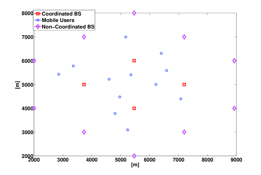
Figure 1: Topology of simulated network.

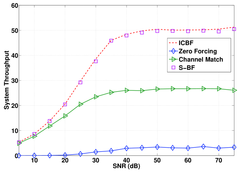
Figure 2: Comparison of system throughput of Different Algorithms. $K=5$, $N=5$, $M=4$. Users $i\in\mathcal{N}_{m}$ uniformly placed within $d_{m,m_{i}}\in[200,~{}1000]$ meters within each BS.

In Fig. 2 and Fig. 4, we consider networks with $N=K=5$ and $N=K=10$, where the the users $i\in\mathcal{N}_{m}$ that are associated with BS $m$ are uniformly placed within $d_{m,m_{i}}\in[200,~{}1000]$ meters. We show the sum rate performance of the S-BF algorithm comparing with the ICBF algorithm in [13] and the non-coordinating schemes where the BSs individually perform zero forcing beamforming and channel matched filter beamforming. In Fig. 4 we consider network with $N=K=5$ and $d_{m,m_{i}}\in[200,~{}300],~{}\forall~{}m,i$. Clearly all the coordinated schemes achieve similar throughput performance, which is significantly higher than the non-coordinated schemes.

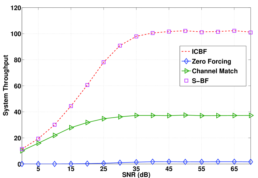
Figure 3: Comparison of system throughput of Different Algorithms. $K=10$, $N=10$, $M=4$. Users $i\in\mathcal{N}_{m}$ uniformly placed within $d_{m,m_{i}}\in[200,~{}1000]$ meters within each BS.

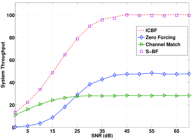
Figure 4: Comparison of system throughput of different Algorithms. $K=5$, $N=5$, $M=4$. Users $i\in\mathcal{N}_{m}$ uniformly placed within $d_{m,m_{i}}\in[200,~{}300]$ meters within each BS.

We then compare the amount of inter-cell information needed for different coordinated schemes. We define the unit of information transfer as the total information needed from the set of coordinated BS for updating the beam vectors for a single BS $m\in\mathcal{M}$. Clearly, in each iteration of the S-BF algorithm, a single unit of information is needed to go through the backhaul network, while in ICBF algorithm, $M$ units of information are needed. In Fig. 6 and Fig. 6, we demonstrate the averaged number of iterations and the averaged total units of information needed for different coordinated schemes until convergence. We observe that the total units of information needed for the proposed SSCA-BF and S-BF algorithms are around $25\%$ less than the ICBF algorithm when $M=4$, and around $40\%$ less when $M=9$. We also emphasize that typically, several inner iterations are needed per outer iteration of ICBF, and we have not count the extra information needed between the BSs and the users in these inner iterations. As a results, in Fig. 6 and Fig. 6 we see that the total iterations needed for ICBF algorithm are close to the S-BF algorithm. In all the simulations presented above, the results are obtained by averaging over $500$ randomly generated user locations and channel realizations.

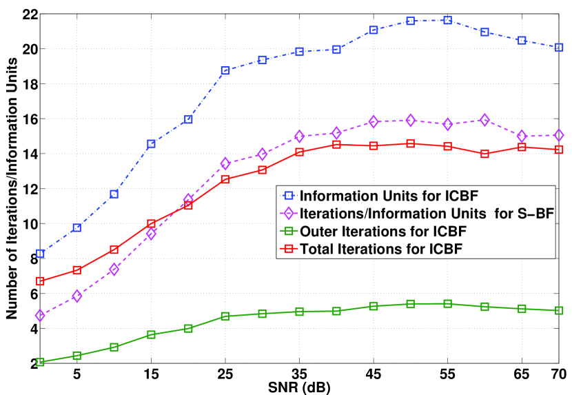
Figure 5: Comparison of the Number of Iterations/Information Units Needed for Convergence. $K=5$, $N=5$, $M=4$.

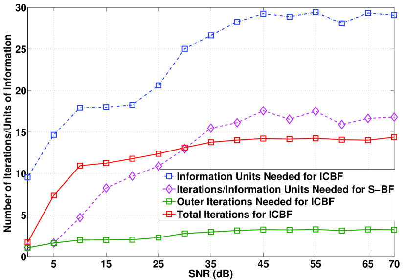
Figure 6: Comparison of the Number of Iterations/Information Units Needed for Convergence. $K=5$, $N=5$, $M=9$.

VI Conclusion

In this correspondence, we study the sum rate maximization problem using beamforming in a multi-cell MISO network. We have explored the structure of the problem and identified a set of lower bounds for the system sum rate. For the case of a single user per cell, we proposed an algorithm that reaches the KKT point of the sum rate maximization problem. For the case of multiple users per cell, we propose and algorithm that achieve high system throughput with reduced backhaul information exchange among the BSs.

References

• [1] G. J. Foschini and M.J. Gans, “On limits of wireless communications in a fading environment when using multiple antennas,” Wireless Personal Communications, vol. 6, no. 3, pp. 311–335, 1998.
• [2] “IEEEstandard for local and metropolitan area networks part 16: Air interface for broadband wireless access systems amendment 3: Advanced air interface,” 2011, IEEE Std 802.16m-2011.
• [3] “Evolved Universal Terrestrial Radio Access (EUTRA) and Evolved Universal Terrestrial Radio Access Network (EUTRAN); overall description,,” 2011, 3GPP TS 36.300, V8.9.0.
• [4] D. Gesbert, S.G. Kiani, A. Gjendemsjø, and G.E. Øien, “Adaptation, coordination, and distributed resource allocation in interference-limited wireless networks,” Proceedings of the IEEE, vol. 95, no. 12, pp. 2393–2409, 2007.
• [5] M.K. Karakayali, G.J. Foschini, and R.A. Valenzuela, “Network coordination for spectrally efficient communications in cellular systems,” IEEE Wireless Communications, vol. 13, no. 4, pp. 56–61, 2006.
• [6] M. Sawahashi, Y. Kishiyama, A. Morimoto, D. Nishikawa, and M. Tanno, “Coordinated multipoint transmission/reception techniques for LTE-advanced,” IEEE Wireless Communications, vol. 17, no. 3, pp. 26–34, 2010.
• [7] J. Zhang, R. Chen, J.G. Andrews, A. Ghosh, and R.W. Heath, “Networked mimo with clustered linear precoding,” IEEE Transactions on Wireless Communications, , no. 8, pp. 1910–1921, 2009.
• [8] A. García Armada, Roberto Corvaja, M. Sánchez-Fernández, and Ana Santos Rodríguez, “MMSE precoding for downlink coordinated base station transmission,” in the Proceedings of IEEE Vehicular Technology Conference, 2011, pp. 1–5.
• [9] H. Sun, W. Fang, and L. Yang, “A novel precoder design for coordinated multipoint downlink transmission,” in the Proceedings of IEEE Vehicular Technology Conference, 2011, pp. 1–5.
• [10] E. Bjornson, R. Zakhour, D. Gesbert, and B. Ottersten, “Cooperative multicell precoding: Rate region characterization and distributed strategies with instantaneous and statistical CSI,” IEEE Trans. on Signal Process., vol. 4658, 2010.
• [11] H. Huh, H. Papadopoulos, and G. Caire, “Multiuser MISO transmitter optimization for intercell interference mitigation,” IEEE Transactions on Signal Processing, vol. 58, pp. 4272–4285, 2010.
• [12] W. Yu, T. Kwon, and C. Shin, “Multicell coordination via joint scheduling beamforming and power spectrum adaptation,” in Proceedings of INFOCOM, 2011.
• [13] L. Venturino, N. Prasad, and X. Wang, “Coordinated linear beamforming in downlink multicell wireless networks,” IEEE Transactions on Wireless Communications, vol. 9, no. 4, pp. 1451–1461, 2010.
• [14] T. M. Cover and J. A. Thomas, Elements of Information Theory, second edition, Wiley, 2005.
• [15] L. Vandenberghe, S. Boyd, and S. P. Wu, “Determinant maximization with linear matrix inequality constraint,” SIAM Journal on Matrix Analysis and Application, vol. 19, no. 2, 1998.
• [16] M. Grant and S. Boyd, “CVX: Matlab software for disciplined convex programming, version 1.21,” Apr. 2011.
• [17] Y. Huang and D. P. Palomar, “Rank-constrained separable semifedinite programming with applications to optimal beamforming,” IEEE Transactions on Signal Processing, vol. 58, 2010.
• [18] A. Wiesel, Y. Eldar, and S. Shamai, “Zero-forcing precoding and generalized inverses,” IEEE Transactions on Signal Processing, vol. 56, no. 1, pp. 4409–4418, 2008.