Robust Max-Product Belief Propagation

Abstract

We study the problem of optimizing a graph-structured objective function under adversarial uncertainty. This problem can be modeled as a two-persons zero-sum game between an Engineer and Nature. The Engineer controls a subset of the variables (nodes in the graph), and tries to assign their values to maximize an objective function. Nature controls the complementary subset of variables and tries to minimize the same objective. This setting encompasses estimation and optimization problems under model uncertainty, and strategic problems with a graph structure. Von Neumann’s minimax theorem guarantees the existence of a (minimax) pair of randomized strategies that provide optimal robustness for each player against its adversary.

We prove several structural properties of this strategy pair in the case of graph-structured payoff function. In particular, the randomized minimax strategies (distributions over variable assignments) can be chosen in such a way to satisfy the Markov property with respect to the graph. This significantly reduces the problem dimensionality. Finally we introduce a message passing algorithm to solve this minimax problem. The algorithm generalizes max-product belief propagation to this new domain.

I Introduction

A two-persons zero-sum game in normal form is specified by an objective (or utility) function ${\cal O}:(x,\theta)\mapsto{\cal O}(x,\theta)$, whereby $x\in{\mathcal{X}}$ is the strategy of the first player (which we shall call by convention the Engineer), while $\theta\in\Theta$ is the strategy of the second player (Nature). Once the strategy pair $(x,\theta)$ is chosen, the Engineer earns from Nature an amount ${\cal O}(x,\theta)$. The two players optimize their strategies with respect to the opposite objective of maximizing (Engineer) or minimizing (Nature) the objective. Zero-sum games capture strategic situations in which agents compete for a fixed, limited pool of resources [21, 3, 17]. Remarkably, they have found broad applicability beyond economic theory, including areas such as online prediction and learning [6], and statistical decision theory [2]. Here statistical estimation is viewed as a game between a Statistician (who tries to design the best statistical procedure) and Nature (who chooses the worst parameters).

Closer to our motivation, a large variety of optimal design problems in engineering can be reduced to maximizing an appropriate objective function. The form of this function is normally dictated by a model of the underlying system, with parameters to be estimated empirically. Of course the parameter estimation process is inherently imprecise and, more importantly, any model of a real system necessarily overlooks a multitude of effects. This remark has motivated the burgeoning fields of robust optimization and robust control [1]. In this context, one considers a family of objective functions $x\mapsto{\cal O}(x;\theta)$, with $x$ the design variables, and $\theta\in\Theta$ a vector of parameters. Rather than designing for a ‘nominal’ $\theta_{*}\in\Theta$, one then tries to maximize the worst case cost $\min_{\theta\in\theta}{\cal O}(x;\theta)$. The problem is hence reduced to a two-players zero-sum game.

Robust optimization theory provides a wealth of structural information, and efficient algorithms for classes of objective functions ${\cal O}(\,\cdot\,,\theta):x\mapsto{\cal O}(x,\theta)$ that are convex in the control variables $x$. The present paper takes a complementary point of view. We assume that both $x$ and $\theta$ take values in high-dimensional, discrete spaces. Explicitly, $x=\underline{x}\in{\mathcal{X}}^{V}$ and $\theta=\underline{\theta}\in\Theta^{F}$ where ${\mathcal{X}}$, $\Theta$ are finite alphabets and $V$, $F$ are finite index sets. Letting $|V|=n$ and $|F|=m$, a pair of pure strategies is specified by two vectors: the Engineer controls variables $\underline{x}=(x_{1},x_{2},\dots,x_{n})$ indexed by the elements of $V$, while Nature controls parameters $\underline{\theta}=(\theta_{1},\theta_{2},\dots,\theta_{n})$. Within this setting we aim at finding strategies for the Engineer which are optimally robust with respect to Nature.

Of course, this general problem is NP-hard, and indeed so even in absence of any adversary (since it includes MaxSat as a special case). Our approach is to exploit simplifications that follow from the underlying factorization structure of the objective function. More precisely, we shall assume that the objective ${\cal O}(\underline{x},\underline{\theta})$ can be expressed as a sum of terms which are local on a graph $G=(V,F,E)$, whereby $V$ is the set of nodes controlled by the Engineer, $F$ the set of nodes controlled by Nature, and $E$ the edge set.

Graph-structured objective functions naturally arise from probabilistic graphical models [15]. In particular, if $\mu(\underline{x})$ is the probability of configuration $\underline{x}$ under a probabilistic graphical model, then $\log\mu(\underline{x})$ is an objective function that factors additively. Hence MAP estimation falls in the class of optimization problems considered here. With a slight abuse of terminology, we shall use the term ‘graphical model’ to refer to general graph-structured objective functions, even if these are not originated from probability distributions.

The application to graphical models also clarifies the need for robustness. Graphical models are particularly effective at expressing complex relationships. Think for instance to the subtle relationships between diseases and symptoms in a medical diagnostic systems [16]. Such relationships are normally modeled through simple parametric families of conditional probabilities (e.g. logit or noisy OR). However, it is not expected that these parametric expressions coincide with the ‘true’ conditional distributions. The only solid justification for this methodology is that the resulting predictions are robust with respect to the details of the model itself. Robustness is therefore implicitly assumed, but has never been carefully investigated and accounted for (but see Section IV for related work).

Apart from the use of graphical models, we achieve significant structural simplification by convexifying the space of strategies, i.e. introducing randomized (mixed) strategies. This is a well established path within game theory. The Engineer has at her disposal a stochastic device generating strategy $\underline{x}\in{\mathcal{X}}^{V}$ with probability $p(\underline{x})$, and plays it, while Nature plays strategy $\underline{\theta}\in\Theta^{F}$ with probability $q(\underline{\theta})$. The Engineer tries to maximize the expected utility $\mathbb{E}_{(p,q)}\{{\cal O}(\underline{x},\underline{\theta})\}$, while Nature tries to minimize the same quantity. A crucial consequence is that the problems faced by the two players become dual linear programs (LPs). In particular, the celebrated Von Neumann’s minimax theorem ensures the existence of a saddle point, i.e. a strategy pair $(p^{*},q^{*})$ such that for any other strategies $p$, $q$

$$\mathbb{E}_{(p,q^{*})}\{{\cal O}(\underline{x},\underline{\theta})\}\leq\mathbb{E}_{(p^{*},q^{*})}\{{\cal O}(\underline{x},\underline{\theta})\}\leq\mathbb{E}_{(p^{*},q)}\{{\cal O}(\underline{x},\underline{\theta})\}\,.$$ (1)

This is equivalent to requiring that $(p^{*},q^{*})$ forms a Nash equilibrium. The saddle point condition implies in particular that the order of play does not matter: $\max_{p}\min_{q}\mathbb{E}_{(p,q)}\{{\cal O}(\underline{x},\underline{\theta})\}=\min_{q}\max_{p}\mathbb{E}_{(p,q)}\{{\cal O}(\underline{x},\underline{\theta})\}$. In words, $p^{*}$ provides to the Engineer optimal robustness against Nature’s adversarial choice, and indeed the same as if this choice was known in advance. Remarkably, the worst-case expected utility of strategy $p^{*}$ is in general strictly larger than the utility of any pure strategy.

Notice that convexification of the strategies space is achieved at the expense of an exponential blow-up in dimensionality. While a pure strategy for the Engineer is a (discrete) vector of length $n$, a mixed strategy is a (probability) vector of length $|{\mathcal{X}}|^{n}$. Hence, by itself, convexification does not reduce the problem complexity.

In the next section we will illustrate key ideas and questions on a simple example, and then describe our general formalism and contributions. In Section III we derive a message passing algorithm, called Robust Max-Product  to construct minimax strategies. Finally, we review related work in Section IV.

II An example and main contributions

a

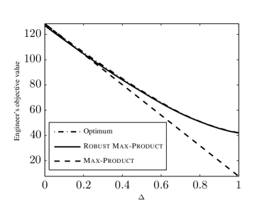
Figure 1: Engineer’s objective vs. $\Delta$ for the Ising model example.

a

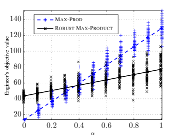
Figure 2: Ising model example; the solid curves indicate the Engineer’s expected payoff and the scattered points show the payoff for random instantiations of mixed strategies. For each value of $\alpha$, there are $50$ random instantiations of mixed strategies.

Ising models. The Ising model is a pairwise graphical model with binary alphabet ${\mathcal{X}}=\{-1,+1\}$. The unnormalized log probability ${\cal O}(\underline{x},\underline{\theta})=\log\mu(\underline{x})+{\rm const.}$ can be written as

$$\begin{split}{\cal O}(\underline{x},\underline{\theta})=\sum_{(i,j)\in E}\psi_{ij}(x_{i}x_{j};\theta_{ij})+\sum_{i\in V}\psi_{i}(x_{i};\theta_{i}),\\ \psi_{ij}(x_{i}x_{j};\theta_{ij})=\theta_{ij}x_{i}x_{j},\;\psi_{i}(x_{i};\theta_{i})=\theta_{i}x_{i}.\end{split}$$ (2)

In practice, the parameters $\underline{\theta}$ are learned from the data and hence are inaccurate. The Engineer’s challenge is to find an strategy $p^{*}(\underline{x})$ which maximize $\mathbb{E}_{(p(\underline{x}),q^{*}(\underline{\theta}))}{\cal O}(\underline{x},\underline{\theta})$ for the worst case distribution $q^{*}$ of the uncertain parameter $\underline{\theta}$.

Minimax strategies depend on the domain of $\underline{\theta}$. We considered a family of models with parameters $h,\Delta\geq 0$. Single variable potentials have $\theta_{i}\!\sim\!U[-h,h]$, i.e., $\theta_{i}$ is uniformly distributed between $-h$ and $h$, and edges belong to two classes: positive and negative. Positive edges have $\theta_{ij}\in\{+1-\Delta,+1,+1+\Delta\}$ while negative edges have $\theta_{ij}\in\{-1-\Delta,-1,-1+\Delta\}$.

Finding minimax strategies for this model is NP-hard, even in the special case of $\Delta=0$, $h=0$. Indeed, when all edges are negative, this reduces to the MAXCUT problem.

We consider a random tree with $n=93$ nodes as the underlying graph and perform the following experiments.

First Experiment: We apply the Robust Max-Product  algorithm derived in Section III to find the Engineer’s optimum strategy, $p^{*}$. We further compare it with the case the Engineer ignores Nature and apply the classical Max-Product  to the graph with nominal values; namely $\theta_{ij}=+1$ on positive edges and $-1$ on negative edges. Finally, in order to check the convergence of Robust Max-Product  , we compute $p^{*}$ by solving the minimax optimization problem in cvx[12]. Note that the latter is computationally much more expensive than the Robust Max-Product  and Max-Product  . Figures 1 summarizes the results for different values of $\Delta$. Robust Max-Product  was run for $100$ iterations. For $\Delta=0$, Max-Product  and Robust Max-Product  are equivalent as Nature has no power. As $\Delta$ increases, Robust Max-Product  performs increasingly better compared to Max-Product  .

Second Experiment: Let $p^{*}$ be the Engineer’s strategy given by Robust Max-Product  algorithm, and let $\tilde{p}^{*}$ be the one obtained by applying Max-Product  considering the nominal values of the parameters. Finally, denote by $q^{*}$ and $\tilde{q}^{*}$, Nature’s best responses against $p^{*}$ and $\tilde{p}^{*}$. In this experiment, we compare the performance of strategies $p^{*}$ and $\tilde{p}^{*}$, when Nature deviates from her optimal strategies $q^{*},\tilde{q}^{*}$. More specifically, Nature’s strategy is chosen to be a mixture of her optimum strategy and the uniform distribution, i.e., $q(\underline{\theta})=(1-\alpha)q^{*}(\underline{\theta})+\alpha|\Theta|^{-m}$ and $\tilde{q}(\underline{\theta})=(1-\alpha)\tilde{q}^{*}(\underline{\theta})+\alpha|\Theta|^{-m}$. Figure 2 illustrates the Engineer’s payoff for the pairs of strategies $(p^{*},q(\underline{\theta}))$ and $(\tilde{p}^{*},\tilde{q}(\underline{\theta}))$, as $\alpha$ varies. Here, $\alpha=0$ corresponds to the case Nature chooses her optimum strategy. Robust Max-Product  outperforms the simple Max-Product  in this regime. As $\alpha$ increases, Nature changes from being adversarial to completely random for $\alpha=1$. Max-Product  outperforms Robust Max-Product  in the latter case, since Nature is no-longer an adversary and one can design for nominal values.

II-A Main contributions

We consider a general bipartite graph (or factor graph) $G=(V,F,E)$, where nodes in $V$ (variable nodes, to be denoted by $i,j,k,\dots$) are controlled by the Engineer, nodes in $F$ (factor nodes, denoted by $a,b,c,\dots$) are controlled by Nature, and $E\subseteq V\times F$ is a set of undirected edges. Given $i\in V$ , the set of its neighbors is denoted by $\partial{i}=\{a\in F:(i,a)\in E\}$. The neighborhood of $a\in F$ , denoted by $\partial{a}$, is defined analogously.

The objective function ${\cal O}:{\mathcal{X}}^{V}\times\Theta^{F}\to{\mathbb{R}}$ factors on graph $G$ if there exists a set of functions $\underline{\psi}=\{\psi_{a}:a\in F\}$, $\psi_{a}:{\mathcal{X}}^{\partial{a}}\times\Theta\to{\mathbb{R}}$ such that

$${\cal O}(\underline{x},\underline{\theta})=\sum_{a\in F}\psi_{a}(\underline{x}_{\partial{a}};\theta_{a}).$$

The functions $\psi_{a}$ are called potentials. There is no loss of generality in assuming $G$ to be bipartite. If two nodes $i$, $j$ controlled by the same player were neighbors, we could replace them by a single node with strategy space ${\mathcal{X}}^{\prime}\equiv{\mathcal{X}}\times{\mathcal{X}}$.

As discussed above, our goal is to find a pair $(p^{*},q^{*})$ where $p^{*}$ is a probability distribution over ${\mathcal{X}}^{V}$, $q^{*}$ a distribution over $\Theta^{F}$, and the pair satisfies the Nash equilibrium condition (1). From the point of view of the Engineer, this amounts to solving the problem

$$p^{*}=\text{\rm{arg}}\max_{p}\min_{q}\mathbb{E}_{(p,q)}{\cal O}(\underline{x},\underline{\theta})\,.$$ (3)

The support $\text{supp}(p)$ of a probability distribution $p$ is the smallest set $S$ such that $p(S^{c})=0$.

Since $\mathbb{E}_{(p,q)}{\cal O}(\underline{x},\underline{\theta})$ is linear both in $p$ and $q$, which belong to the simplex, (3) is equivalent to an LP problem. However, the dimensionality of this problem is exponential in the graph size: even writing down the strategy takes exponential time. The following result plays a key role in our approach.

Theorem II.1.

In problem (3), without loss of generality, we can assume that the Engineer’s strategy is a Markov Random Field (MRF) with factor graph $G$, and that Nature chooses a product distribution. Explicitly, the Engineer’s strategy can be assumed to take the form $p^{*}(\underline{x})=\prod_{a\in F}f_{a}(\underline{x}_{\partial{a}})$, while Nature’s strategy takes the form $q^{*}(\underline{\theta})=\prod_{a\in F}g_{a}(\theta_{a})$.

Proof:

Note that the Engineer’s pay off is given by

$$\mathbb{E}_{(p(\underline{x}),q(\underline{\theta}))}\sum_{a\in F}\psi_{a}(\underline{x}_{\partial{a}};\theta_{a})=\sum_{a\in F}\mathbb{E}_{q_{a}(\theta_{a})}\mathbb{E}_{p_{a}(\underline{x}_{\partial{a}})}\psi_{a}(\underline{x}_{\partial{a}};\theta_{a}).$$

Therefore, only the marginals $q_{a}(\theta_{a})$ of the Nature’s distribution play role in the pay off. Hence, we can assume that Nature has a product distribution $q(\underline{\theta})=\prod_{a\in F}q_{a}(\theta_{a})$.

Similarly, only the marginals $p_{a}(\underline{x}_{\partial{a}})$ appears in the pay off. Thereby, without loss of generality we can assume that the Engineer’s distribution is an MRF with respect to $G$. This follows from the fact that for all factor graphs $G$ and for all joint distributions $p(\underline{x})$, there exists a distribution $\tilde{p}(\underline{x})$ that is representable as an MRF with graph $G$ such that $p_{a}(\underline{x}_{\partial{a}})=\tilde{p_{a}}(\underline{x}_{\partial{a}})$ [17]. ∎

Notice that, for a graph $G$ with bounded degree, a MRF can be specified by $O(|V|)$ parameters. In particular, the MRF is completely specified by the marginals $p_{a}(\underline{x}_{\partial a})$. We then reformulate the minimax problem as the one of computing the minimax marginals $\{p_{a}^{*}\}_{a\in F}$. By definition, these belong to the so-called marginal polytope [22]

$${\rm MARG}(G)\equiv\Big{\{}\{p_{a}\}_{a\in F} \Big{|}\;p_{a}(\underline{x}_{\partial{a}})=\sum_{\underline{x}_{V\backslash\partial{a}}}p(\underline{x}),$$

$$\text{ for some distribution }p(\underline{x})\Big{\}}\,.$$

Problem 3 can therefore be restated as an LP over ${\rm MARG}(G)$:

$$\begin{split}&\underset{p_{a}(\underline{x}_{\partial{a}})}{\text{maximize}}\quad\sum_{a\in F}\underset{\theta_{a}}{\min}\Big{[}\sum_{\underline{x}_{\partial a}}p_{a}(\underline{x}_{\partial{a}})\psi_{a}(\underline{x}_{\partial a};\theta_{a})\Big{]},\\ &\text{s.t.}\quad\quad\quad\quad\{p_{a}\}_{a\in F}\in{\rm MARG}(G)\,.\end{split}$$ (4)

Here we used the fact that the $\min$ over $q$ in the simplex is necessarily achieved at one extremal point, i.e. at a pure strategy. In general, ${\rm MARG}(G)$ does not possess a polynomial separation oracle and therefore this problem is not tractable. Instead, we relax it to the set of locally consistent marginals on $G$, denoted by ${\rm LOC}(G)$

$$\begin{split}&{\rm LOC}(G)=\\ &\Bigg{\{}\{p_{a}\}_{a\in F}\;\begin{array}[]{|ll}\exists p_{i}(x_{i}):p_{i}(x_{i})\geq 0,&\underset{x_{i}}{\sum}p_{i}(x_{i})=1\\ p_{a}(\underline{x}_{\partial{a}})\geq 0,&\underset{\underline{x}_{\partial{a}\backslash i}}{\sum}p_{a}(\underline{x}_{\partial{a}})=p_{i}(x_{i})\end{array}\Bigg{\}}.\end{split}$$ (5)

We then have the following relaxation of problem (LABEL:eqn:minimax) to the local polytope.

$$\begin{split}(\text{P}_{0}):\quad&\underset{p_{a}(\underline{x}_{\partial{a}})}{\text{maximize}}\quad\sum_{a\in F}\underset{\theta_{a}}{\min}\Big{[}\sum_{\underline{x}_{\partial a}}p_{a}(\underline{x}_{\partial{a}})\psi_{a}(\underline{x}_{\partial a};\theta_{a})\Big{]}\,,\\ &\text{s.t.}\quad\quad\quad\quad\{p_{a}\}_{a\in F}\in{\rm LOC}(G)\,.\end{split}$$ (6)

If $G$ is a tree, then $\text{\rm{LOC}}(G)\equiv\text{\rm{MARG}}(G)$ and therefore this relaxation is exact.

III Algorithm

Here, we first present the alternating direction method of multipliers (ADMM) [10], [11] algorithm for solving convex optimization problems and state a general result regarding its convergence properties. Subsequently, we show how the optimization problem ${(\text{P}_{0})}$ can be transformed to conform with the general form for the ADMM algorithm. We derive the Robust Max-Product  algorithm from the transformed variant of the problem ${(\text{P}_{0})}$ and obtain convergence guarantees using the result stated for the general case of ADMM algorithms.

III-A ADMM Algorithm

What follows is a short presentation of the ADMM algorithm and its properties. The reader interested in a more comprehensive treatment can refer to [4]. Consider the optimization problem

$$\begin{split}&\underset{x\in{\mathbb{R}}^{n},z\in{\mathbb{R}}^{m}}{\text{minimize}}\quad f(x)+g(z),\\ &\text{s.t.}\quad\quad\quad\quad Ax-z=0.\end{split}$$ (7)

where $A\in{\mathbb{R}}^{p\times n}$. The augmented Lagrangian for this problem is defined as

$$L_{\rho}(x,z,y)=f(x)+g(z)+y^{T}(Ax-z)+\frac{1}{2}\rho\|Ax-z\|_{2}^{2}.$$ (8)

with $\rho>0$ a parameter and $\|\cdot\|_{2}$ indicating the $\ell_{2}$ norm. The ADMM algorithm tries to solve the above optimization problem by starting from some initial estimates $(z^{(0)},y^{(0)}=0)$ and performing the following iteration

$$\begin{split}x^{(t+1)}&=\underset{x}{{\text{\rm{arg}}\!\min}}\;L_{\rho}(x,z^{(t)},y^{(t)})\,,\\ z^{(t+1)}&=\underset{z}{{\text{\rm{arg}}\!\min}}\;L_{\rho}(x^{(t+1)},z,y^{(t)})\,,\\ y^{(t+1)}&=y^{(t)}+\rho(Ax^{(t+1)}-z^{(t+1)}).\end{split}$$ (9)

The update rules in (9) closely resemble the dual gradient descent method where the dual is obtained from the augmented Lagrangian. This indeed is the gist of the method of multipliers. Despite the fact that the primal optimization is done in two steps and the augmented Lagrangian is used in place of the Lagrangian, the iteration (9) provably converges to the solution of 7. Formally, assume the optimization problem (7) has a finite optimum value $p^{*}$. We say the Lagrangian $L(x,z,y)$ has a saddle point $(x^{*},z^{*},y^{*})$ if $L(x^{*},z^{*},y)\leq L(x^{*},z^{*},y^{*})\leq L(x,z,y^{*})$ for all $x$, $z$, and $y$. Then the following theorem holds.

Theorem III.1.

([10] Theorem 3.1, [8] Theorem 8, [4] Section 3.2) Assume that the extended real valued functions $f(x)$ and $g(z)$ are closed, proper, and convex and the un-augmented Lagrangian $L_{0}(x,z,y)$ has a saddle point. Then

$$\lim_{t\to\infty}f(x^{(t)})+g(z^{(t)})\to p^{*}$$

$$\lim_{t\to\infty}Ax^{(t)}-z^{(t)}\to 0$$

$$\lim_{t\to\infty}y^{(t)}\to y^{*}$$ (10)

III-B Robust Max-Product  Algorithm

TABLE I: Robust Max-Product  Algorithm

 
Robust Max-Product:
 
Input: Factor graph $G(V,F,E)$, potential functions $\{\psi_{a}(\underline{x}_{\partial a},\theta_{a}\}_{a\in F}$
Output: Local marginals $\{p_{a}(\underline{x}_{\partial a})\}_{a\in F}$
${\bf 1.}$ Initialize:

$$\qquad u^{(0)}_{ai}(x)=0,\quad\forall\;(a,i)\in E,\;x\in{\mathcal{X}}\hskip 227.62204pt$$

$$\qquad p^{(0)}_{i}(x)=\frac{1}{|{\mathcal{X}}|},\quad\forall\;i\in V,\;x\in{\mathcal{X}}$$

${\bf 2.}$ Update until convergence:
 At the factor nodes:

$$\begin{array}[]{l l l}\qquad\left\{p_{a}^{(t+1)},\lambda_{a}^{(t+1)}\right\}=&\underset{p_{a},\lambda_{a}}{{\text{\rm{arg}}\!\min}}&\lambda_{a}+\frac{\rho}{2}\underset{\begin{subarray}{c}i\in\partial a\\ x_{i}\in{\mathcal{X}}\end{subarray}}{\sum}\left(\underset{\underline{x}_{\partial{a}\backslash i}}{\sum}p_{a}(\underline{x}_{\partial{a}\backslash i};x_{i})-p_{i}^{(t)}(x_{i})-u_{ai}^{(t)}(x_{i})\right)^{2}\\ \vspace{10pt}&{\rm s.t.}&\lambda_{a}+\sum_{\underline{x}_{\partial{a}}}p_{a}(\underline{x}_{\partial{a}})\psi_{a}(\underline{x}_{\partial{a}};\theta_{a})\geq 0,\quad\forall{a,\theta_{a}}\\ \vspace{10pt}&&p_{a}(\underline{x}_{\partial{a}})\geq 0,\hskip 108.12054pt\forall\underline{x}_{\partial a}\in{\mathcal{X}}^{|\partial a|}\\ \end{array}\hskip 113.81102pt$$

At the variable nodes:

$$\qquad p_{i}^{(t+1)}=\Pi_{{\cal S}^{|{\mathcal{X}}|-1}}\left(\frac{1}{|\partial i|}\underset{a\in\partial i}{\sum}\left\{\underset{\underline{x}_{\partial{a}\backslash i}}{\sum}p^{(t)}_{a}(\underline{x}_{\partial{a}\backslash i};\cdot)-u_{ai}^{(t)}(\cdot)\right\}\right),$$

$$\qquad u_{ai}^{(t+1)}(x_{i})=u_{ai}^{(t)}(x_{i})+\underset{\underline{x}_{\partial{a}\backslash i}}{\sum}p^{(t+1)}_{a}(\underline{x}_{\partial{a}\backslash i};x_{i})-p_{i}^{(t+1)}(x_{i})\qquad\forall\;i,\;a\in\partial i,\;x_{i}\in{\mathcal{X}}.\hskip 113.81102pt$$

${\bf 3.}$ Return: $\{p_{a}\}_{a\in F}$.
 

Note that the epigraph form of the optimization problem ${(\text{P}_{0})}$ is given by

$$\begin{array}[]{l l r}{\text{minimize}}&\underset{a\in F}{\sum}\lambda_{a}&\\ \text{s.t.}&\lambda_{a}+\underset{\underline{x}_{\partial{a}}}{\sum}p_{a}(\underline{x}_{\partial{a}})\psi_{a}(\underline{x}_{\partial{a}};\theta_{a})\geq 0,&\forall{a,\theta_{a}}\\ &p_{i}(x_{i})=\underset{\underline{x}_{\partial{a}\backslash i}}{\sum}p_{a}(\underline{x}_{\partial{a}}),&\forall{(i,a)\in E,x_{i}}\\ &\sum_{x_{i}}p_{i}(x_{i})=1,&\forall{i\in V}\\ &p_{a}(\underline{x}_{\partial{a}})\geq 0,&\forall{(i,a)\in E,\underline{x}_{\partial{a}}}\\ &p_{i}(x_{i})\geq 0,&\forall{i\in V,x_{i}}\\ &&\end{array}$$ (11)

where the minimization is over $\{\lambda_{a}\}_{a\in F},\{p_{a}\}_{a\in F},\{p_{i}\}_{i\in V}$ and ${\rm LOC}(G)$ is represented in terms of the set of marginals. Define the indicator function $\mathbb{I}(\cdot)$ as

$$\mathbb{I}(x)=\left\{\begin{array}[]{l l}0&\text{if }x=\text{TRUE},\\ \infty&\text{if }x=\text{FALSE}.\end{array}\right.$$ (12)

Furthermore, let $f(\{\lambda_{a}\}_{a\in F},\{p_{a}\}_{a\in F})=\sum_{a\in F}\tilde{f}(\lambda_{a},p_{a})$ and $g(\{p_{i}\}_{i\in V})=\sum_{i\in V}\tilde{g}(p_{i})$ whereby $\tilde{f}(\lambda_{a},p_{a})$ and $\tilde{g}(p_{i})$ are defined as

$$\tilde{f}(\lambda_{a},p_{a}) =\lambda_{a}+\sum_{\theta_{a}\in\Theta}{\mathbb{I}}(\lambda_{a}+\sum_{\underline{x}_{\partial{a}}}p_{a}(\underline{x}_{\partial{a}})\psi_{a}(\underline{x}_{\partial{a}};\theta_{a})\geq 0)$$

$$\;\;+\sum_{\underline{x}_{\partial a}\in{\mathcal{X}}^{|\partial a|}}{\mathbb{I}}(p_{a}(\underline{x}_{\partial{a}})\geq 0),$$ (13)

and

$$\tilde{g}\left(p_{i}\right)={\mathbb{I}}(p_{i}\in{\cal S}^{|{\mathcal{X}}|-1}).$$ (14)

Here, ${\cal S}^{|{\mathcal{X}}|-1}$ is the $|{\mathcal{X}}|-1$ dimensional simplex and $p_{a}$ and $p_{i}$ are the $|{\mathcal{X}}|^{|\partial a|}$ and $|{\mathcal{X}}|$ dimensional real vectors respectively. It is easy to see that the extended real valued functions

$$f :{\mathbb{R}}^{|F|+\sum_{a\in F}|{\mathcal{X}}|^{|\partial a|}}\to(-\infty,+\infty]$$

$$g :{\mathbb{R}}^{|V||{\mathcal{X}}|}\to(-\infty,+\infty]$$

are closed, convex, and proper.

Using the functions $f$ and $g$, the optimization problem (11) can be restated as

$${(\text{P})}:$$

$$\begin{array}[]{l l l }{\text{minimize}}&f(\{\lambda_{a}\}_{a\in F},\{p_{a}\}_{a\in F})+g(\{p_{i}\}_{i\in V})&\\ \text{s.t.}&p_{i}(x_{i})=\underset{\underline{x}_{\partial{a}\backslash i}}{\sum}p_{a}(\underline{x}_{\partial{a}\backslash i};x_{i}),&\forall(a,i)\in E,\\ &&\forall x_{i}\in{\mathcal{X}},\end{array}$$

where the minimization is over $\{\lambda_{a}\}_{a\in F}$, $\{p_{a}\}_{a\in F}$, and $\{p_{i}\}_{i\in V}$. Optimization problem ${(\text{P})}$ follows the form of the general problem in Eq. (7) and can be solved using the ADMM algorithm. The augmented Lagrangian for problem ${(\text{P})}$ can be written as

$$\begin{split}&L_{\rho}\left(\{\lambda_{a}\}_{a\in F},\{p_{a}\}_{a\in F},\{p_{i}\}_{i\in V},\{u_{ai}\}_{(a,i)\in E}\right)=\\ &\quad\qquad\sum_{a\in F}\tilde{f}(\lambda_{a},p_{a})+\sum_{i\in V}\tilde{g}\left(p_{i}\right)\\ &\quad+\sum_{(a,i)\in E,x_{i}\in{\mathcal{X}}}u_{ai}(x_{i})\,\Big{(}p_{i}(x_{i})-\sum_{\underline{x}_{\partial{a}\backslash i}}p_{a}(\underline{x}_{\partial{a}\backslash i};x_{i})\Big{)}\\ &\quad+\sum_{(a,i)\in E,x_{i}\in{\mathcal{X}}}\rho\,\Big{(}p_{i}(x_{i})-\sum_{\underline{x}_{\partial{a}\backslash i}}p_{a}(\underline{x}_{\partial{a}\backslash i};x_{i})\Big{)}^{2},\end{split}$$ (15)

where $\rho$ is a parameter and $u_{a,i}(x_{i})$ are the dual variables. Notice that the special form of the constraint results in the quadratic penalty being block separable in $\{p_{a}\}_{a\in F}$. Furthermore, the function $f$ is also block separable in $\{p_{a}\}_{a\in F}$, as well. Similarly, the quadratic penalty and the function $g$ are separable in $\{p_{i}\}_{i\in V}$. These facts enable us to further decompose the first two steps of the ADMM iteration (Eq. (9)) and perform the optimization at the corresponding check and variable node locally. The resulting algorithm is presented in Table I.

III-C Convergence of the Robust Max-Product  Algorithm

a

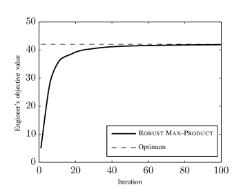
Figure 3: Engineer’s objective vs. iteration.

a

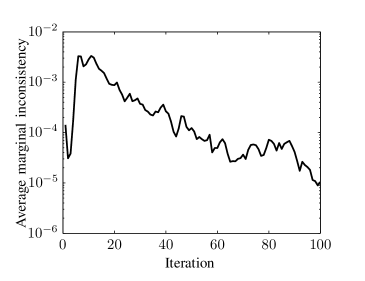
Figure 4: Average marginal inconsistency vs. iteration.

For $(a,i)\in E$, $x_{i}\in{\mathcal{X}}$ and local marginals $\{p_{a}\}_{a\in F}$, $\{p_{i}\}_{i\in V}$, define the marginal inconsistency residual $r_{ai}(x_{i})$ as

$$r_{ai}(x_{i})=p_{i}(x_{i})-\sum_{\underline{x}_{\partial{a}\backslash i}}{p_{a}(\underline{x}_{\partial{a}\backslash i};x_{i})}.$$ (16)

Let $\underline{r}\in\mathbb{R}^{|E|\times|{\mathcal{X}}|}$ be the vector of residuals defined as $\underline{r}=(\{r_{ai}(x_{i})\}_{(a,i)\in E,x_{i}\in{\mathcal{X}}})$. In particular, let $\underline{r}^{(t)}$ be the marginal inconsistency residual at iteration $t$ of the Robust Max-Product  algorithm.

Define ${\cal C}^{(t)}=\sum_{a\in F}\lambda_{a}^{(t)}$, the cost function at iteration $t$ of the Robust Max-Product  algorithm and let ${\cal C}^{*}$ be the optimum value of the optimization problem (6). Figures 3 and 4 show ${\cal C}^{(t)}$ and $\frac{1}{|E||{\mathcal{X}}|}\|\underline{r}^{(t)}\|_{1}$ as a function of $t$ (iteration) for the Ising model described in Section II with $\Delta=1$. Figure 4 shows that the marginals quickly become nearly consistent while Fig 3 demonstrates that the objective value converges to the optimum value as number of iteration increases to a modest number.

The following theorem provides theoretical guarantees for the behavior observed in Figures 3 and 4. In particular, it states that the sequence of local marginals in the Robust Max-Product  algorithm converges to a set of locally consistent marginals that achieves the optimum payoff for the Engineer.

Theorem III.2.

For any graph $G(F,V,E)$ and set of potential functions $\{\psi_{a}(\underline{x}_{\partial a})\}_{a\in F}$ the followings hold.

• $\underset{t\to\infty}{\lim}\;\underline{r}^{(t)}=\underline{0}.$

• $\underset{t\to\infty}{\lim}\;{\cal C}^{(t)}={\cal C}^{*}.$

The proof of this theorem can be obtained by applying the result of the following lemma to Theorem III.1.

Lemma III.1.

. For any graph $G(F,V,E)$ and potential functions $\{\psi_{a}(\underline{x}_{\partial a})\}_{a\in F}$, the optimization problem (6) is feasible. Furthermore, there exist $\{\lambda_{a}^{*}\}_{a\in F}$, $\{p_{a}^{*}\}_{a\in F}$, $\{p_{i}^{*}\}_{i\in V}$, and $\{u_{ai}\}_{(a,i)\in E}^{*}$ such that $(\{\lambda_{a}^{*}\}_{a\in F}$, $\{p_{a}^{*}\}_{a\in F}$, $\{p_{i}^{*}\}_{i\in V}$, $\{u_{ai}\}_{(a,i)\in E}^{*})$ is a saddle point of the augmented Lagrangian (15) with $\rho=0$ and $\sum_{a\in F}\lambda_{a}^{*}={\cal C}^{*}$.

Proof.

Consider the optimization problem in Eq. (11). First note that given the potential functions $\{\psi_{a}(\underline{x}_{\partial a})\}_{a\in F}$ are bounded, this problem has a strictly feasible point. Also it is a linear program. Hence the strong duality holds by Slater’s theorem [5] and the Lagrangian has a saddle point. Let $\{\lambda_{a}^{*}\}_{a\in F},\{p_{a}^{*}\}_{a\in F},\{p_{i}^{*}\}_{i\in V}$ be the values of the primal variables at this saddle point. Similarly, let $\{u_{ai}^{*}\}_{(a,i)\in E}$ be the values of the dual variables corresponding to the constraints $p_{i}(x_{i})=\sum_{\underline{x}_{\partial{a}\backslash i}}p_{a}(\underline{x}_{\partial{a}})$ at this saddle point. Then $\{\lambda_{a}^{*}\}_{a\in F},\{p_{a}^{*}\}_{a\in F},\{p_{i}^{*}\}_{i\in V}$ are primal optimal for (11). In particular, $\sum_{a\in F}\lambda_{a}^{*}={\cal C}^{*}$. Furthermore, it is easy to see that$(\{\lambda_{a}^{*}\}_{a\in F},\{p_{a}^{*}\}_{a\in F},\{p_{i}^{*}\}_{i\in V},\{u_{ai}^{*}\}_{(a,i)\in E})$ is a saddle point of the Lagrangian in Eq. (15) with $\rho=0$.

∎

IV Related work

Several groups investigated the impact of graphical model structure on the computational properties of Nash equilibria [14, 18, 7, 9]. In particular, Ortiz and Kearns [18] proposed a message passing algorithm (called NashProp) to find Nash equilibria. However, as shown in [9], the problem of computing Nash equilibria is PPAD-complete even on trees. Within graphical games studied in this literature, a different player controls each vertex of a graph, and a game is played along each edge. A single player has at her disposal only a small number of pure strategies (typically two), and the problem complexity arises because of the large number of players.

Let us emphasize that the present paper studies a very different class of models. We consider a small fixed number of players (indeed in this paper only two players), but each of them has at her disposal a large number of pure strategies. The problem complexity is due to the strategies proliferation.

The motivation for focusing on two-players zero-sum games came from their relevance to optimization and inference under model uncertainty. A few authors [13, 20] have already analyzed the sensitivity of message passing algorithms to model uncertainty. However these studies assumed a probability distribution over model parameters, which is very restrictive in a high-dimensional setting, or carried out a perturbation analysis, without constructing more robust algorithms.

ADMM and many related algorithms (Uzawa’s algorithm, Douglas-Rachford splitting, proximal method, Bregman iterative methods, etc.) have been around for a few decades. However, recent years have seen a surge of interest in these algorithms in many fields. The reader can refer to [4] for many examples in the field of statistical learning. Closer to the spirit of this paper, [19] uses the technique of Bregman projection to obtain fractional solution for the maximum a posteriori probability (MAP) problem in graphical models. The problem addressed in this paper is fundamentally different from this work in that we consider the case of adversarial uncertainty in the model.

References

- [1] A. Ben-Tal, L. E. Ghaoui, and A. Nemirovski. Robust Optimization. Princeton University Press, Princeton, 2009.
- [2] J. O. Berger. Statistical Decision Theory and Bayesian Analysis. Springer, New York, 1985.
- [3] K. Binmore. Playing for Real: A Text on Game Theory. Oxford University Press, Oxford, UK, 2007.
- [4] S. Boyd, N. Parikh, E. Chu, B. Peleato, and J. Eckstein. Distributed optimization and statistical learning via the alternating direction method of multipliers. Machine Learning, 3(1):1–123, 2010.
- [5] S. Boyd and L. Vandenberghe. Convex Optimization. Cambridge University Press, Cambridge, 2004.
- [6] N. Cesa-Bianchi and G. Lugosi. Prediction, Learning, and Games. Cambridge University Press, Cambridge, UK, 2006.
- [7] C. Daskalakis and C. H. Papadimitriou. Computing pure Nash equilibria in graphical games via Markov Random Fields. In Proc. of the 7th ACM conference on Electronic Commerce, pages 91–99, 2006.
- [8] J. Eckstein and D. Bertsekas. On the douglas—rachford splitting method and the proximal point algorithm for maximal monotone operators. Mathematical Programming, 55(1):293–318, 1992.
- [9] E. Elkind, L. Goldberg, and P. Goldberg. Nash equilibria in graphical games on trees revisited. In Proceedings of the 7th ACM conference on Electronic commerce, pages 100–109, 2006.
- [10] D. Gabay and B. Mercier. A dual algorithm for the solution of nonlinear variational problems via finite element approximation. Computers & Mathematics with Applications, 2(1):17–40, 1976.
- [11] R. Glowinski and A. Marroco. Sur l’approximation, par éléments finis d’ordre un, et la résolution, par penalisation-dualité, d’une classe de problèmes de dirichlet non linéaires. Rev. Franc. Automat. Inform. Rech. Operat., 9:41–76, 1975.
- [12] M. Grant and S. Boyd. CVX: Matlab software for disciplined convex programming, version 1.21. http://cvxr.com/cvx, Apr. 2011.
- [13] A. Ihler, J. W. F. III, and A. S. Willsky. Loopy belief propagation: Convergence and effects of message errors. J. Mach. Learn. Res., 6:905–936, 2005.
- [14] M. Kearns. Graphical games. In Nisan, Roughgarden, Tardos, and Vazirani, editors, Algorithmic Game Theory. Cambridge University Press, 2007.
- [15] D. Koller and N. Friedman. Probabilistic Graphical Models: Principles and Techniques. The MIT Press, Cambridge, MA, 2009.
- [16] P. Lucas, L. van der Gaag, and A. Abu-Hannac. Bayesian networks in biomedicine and health-care. Artif. Intelligence in Medicine, 30:201–214, 2004.
- [17] N. Nisan, T. Roughgarden, E. Tardos, and V. V. Vazirani. Algorithmic Game Theory. Cambridge University Press, New York, NY, USA, 2007.
- [18] L. E. Ortiz and M. Kearns. Nash propagation for loopy graphical games. In In Neural Information Processing Systems, pages 793–800. MIT Press, 2003.
- [19] P. Ravikumar, A. Agarwal, and M. Wainwright. Message-passing for graph-structured linear programs: Proximal methods and rounding schemes. The Journal of Machine Learning Research, 11:1043–1080, 2010.
- [20] L. Varshney. Performance of LDPC Codes Under Noisy Message-Passing Decoding. In IEEE Information Theory Workshop, pages 178–183, Tahoe City, CA, 2007.
- [21] J. von Neumann and O. Morgenstern. Theory of Games and Economic Behavior. Princeton University Press, Princeton, 2007.
- [22] M. Wainwright and M. I. Jordan. Graphical models, exponential families, and variational inference. Found. Trends Mach. Learn., 1:1–305, 2008.