Linearized Auxiliary fields Monte Carlo: efficient sampling of the fermion sign

Abstract

We introduce a method that combines the power of both the lattice Green function Monte Carlo (LGFMC) with the auxiliary field techniques (AFQMC), and allows us to compute exact ground state properties of the Hubbard model for $U\lesssim 4t$ on finite clusters. Thanks to LGFMC one obtains unbiased zero temperature results, not affected by the so called Trotter approximation of the imaginary time propagator $e^{-H\tau}$. On the other hand the AFQMC formalism yields a remarkably fast convergence in $\tau$ before the fermion sign problem becomes prohibitive. As a first application we report ground state energies in the Hubbard model at $U/t=4$ with up to one hundred sites.

After several years of scientific effort, based on advanced analitycal and numerical methods, only very few properties of the 2D Hubbard model have been settled. The 2D Hubbard model is defined in a square lattice containing a finite number $L$ ($N$) of sites (electrons):

$$H=-t\sum_{<i,j>,\sigma}c^{{\dagger}}_{i,\sigma}c_{j,\sigma}+U\sum_{i}n_{i}^{\uparrow}n_{i}^{\downarrow}$$ (1)

with standard notations. In the thermodinamic limit, namely for $L\to\infty$ at given density $\rho=N/L$ fundamental issues such as the existence of a ferromagnetic phase at large $U/t$ ratio and/or the stability of an homogeneous ground state with possible d-wave supoerconducting properties are still highly debated, as several approximate numerical techniques lead to controversial and often conflicting results. This situation is particularly embarazzing, since recent progress in the realization of fermionic optical lattices could lead soon to the experimental realization of the fermionic Hubbard model, apparently much before we will reach a consensus among the different theoretical and numerical techniques.

Method: In LGFMCldmc , the main property used to compute the ground state $\psi_{0}$ of a many body Hamiltonian $H$, is the iterative application of a linearized Green’s function:

$$G=\Lambda I-{H}$$ (2)

to an initial wave function $\psi$ by a stochastic method, namely $\psi_{0}=\lim\limits_{n\to\infty}G^{n}|\psi\rangle$. Here $I$ is the identity matrix and $\Lambda$ is a suitably large constant. This is possible because the application of $G$ to a given configuration $|x\rangle$, where electrons have definite positions and spins, can be expressed as a sum of a finite number of independent configurations. Namely the number of non zero matrix elements $G_{x^{\prime},x}=\langle x^{\prime}|G|x\rangle$ for given $x$ is affordable ($\propto L$), though the Hilbert space is exponentially large with $L$. For large $n$ it is possible to sample the ground state wave function $\psi_{0}(x)=\langle x|\psi_{0}\rangle$ and its correlation functions. This method can be improved by the so called importance sampling, yielding a much more efficient algorithm: the matrix elements of $G$ are scaled by means of the so called guiding function $\psi_{g}(x)$:

$$\bar{G}_{x^{\prime},x}=\psi_{g}(x^{\prime})G_{x^{\prime},x}/\psi_{g}(x)$$ (3)

This method allows the calculation of exact ground state properties without any approximation other than (i) finite $L$ and (ii) statistical errors. The latter may be particularly large with fermionic systems, due to the unfamous ”sign problem”, a limitation that is usually much severe, if not prohibitive, for this type of approach. We remark also that, in LGFMC, one can work with infinite $\Lambda$caprio and sample the many body propagator $e^{-H\tau}=\lim\limits_{\Lambda\to\infty}({G\over\Lambda})^{n}$ with a similar computational effort, despite $n=\tau\Lambda\to\infty$ in this limit. Moreover, since the projection time $\tau$ is proportional to the length of the Monte Carlo simulation, converged ground state properties are easily obtained after the equilibration time, and the limit $\tau\to\infty$ is basically achieved without any particular effort when there is no sign problem.

Another important stochastic method that is quite popular for the Hubbard model is based on AFQMChirsch ; canieporci and the algebra of one body propagators. The basic property used in this approach is that a one body operator $U$, when applied to a Slater determinant $|D\rangle$, generates again a Slater determinant $|D^{\prime}\rangle=U|D\rangle$, that is easy to evaluate. Obviously, by the above definition, the product of several one-body propagators remains a one-body propagator, and the computation is always feasible for a finite number of them. Indeed, within AFQMC, the many body propagator $e^{-H\tau}$ is conveniently written as a superposition of time dependent one body propagators $U_{[\sigma]}(\tau,0)=U_{\sigma}(t_{L_{\tau}})\cdots U_{\sigma}(t_{1})$ after the introduction of discrete Hubbard-Stratonovich time-dependent auxiliary fields $\sigma_{i}(t_{j})=\pm 1$ defined in all the $L$ lattice sites and a finite number of discrete imaginary times $t_{j}=j\tau/L_{\tau}$ $j=1,\cdots,L_{\tau}$. Thus $e^{-H\tau}|\psi\rangle=\sum\limits_{\sigma}U_{\sigma}(\tau,0)|\psi\rangle$ for large imaginary time gives formally the exact ground state wave function and can be computed by Monte Carlo sampling of the auxiliary fields $\sigma_{i}(t_{j})=\pm 1$.hirsch At variance of the LGFMC technique, it is not simple to avoid the error due to the discretization in time of the propagator-usually called Trotter error- and all the results require a careful and often boring extrapolation both in $\tau\to\infty$ and $L_{\tau}\to\infty$. By contrast, within AFQMC, the sign problem is much less severe for two main reasons, (i) for $U=0$ the method is exact and one does not need any random sampling, (ii) at half-filling or with negative $U$ the method is not affected by the ”sign problem”.

In the following we propose to combine the power of the two methods, by taking the best of the two approaches in what we name Linearized Auxiliary fields Monte Carlo (LAQMC). From AFQMC we take the advantage of a much less severe sign problem and from LGFMC the exact imaginary time projection will be available in a rigorous and simple way. The latter achievement has been made recently possible also within the so called ”diagrammatic” Monte Carloprokovev ; lichtnestein , but only within the reasonable assumption that the diagrammatic perturbation serie converges.

In order to define this new approach we use that the lattice Green function (2) of the Hubbard model can be written exactly as a finite sum of one body propagators $U_{i}$, with an approach that is similar to the conventional auxiliary field technique, where instead of splitting up the many propagator $\exp(-\tau H)$ we focus on its linearized expression given by $G$:

$$G=\Lambda I-H=\sum_{i=1}^{p}a_{i}U_{i}$$ (4)

where the coefficients $a_{i}\geq 0$ and the $U_{i}$ will be defined later on and $p=4L$ for the Hubbard model. The above identity can be generally fullfilled for any reasonable many-body Hamiltonian by using a number $p$ of one-body propagators that scales at most as $L^{2}$. For the Hubbard model we obtain after simple algebra:

$$\Lambda = \Gamma_{U}(e^{\lambda}+e^{-\lambda}-2)N+\sum\limits_{i=1}^{p}a_{i}$$

$$U_{i} = e^{-\gamma_{i}c^{{\dagger}}_{k_{i},\sigma_{i}}c_{k_{i},\sigma_{i}}}~{}~{}i=1,\cdots 2L$$

$$U_{i+5/2L\pm L/2} = e^{\pm\lambda(n_{i}^{\uparrow}-n_{i}^{\downarrow})}~{}~{}i=1,\cdots L$$

where, in order to satisfy Eq.(4):

$$a_{i}(e^{-\gamma_{i}}-1) = -\epsilon_{k_{i}}~{}~{}~{}i\leq 2L$$ (5)

$$2a_{i}(e^{\lambda}-1)(e^{-\lambda}-1) = -U~{}~{}~{}~{}i>2L$$ (6)

and $\epsilon_{k^{i}}=-2t(\cos(k_{x}^{i})+\cos(k_{y}^{i}))$ is the $U=0$ band and $k^{i}$ label all the $2L$ independent $k$ vectors of the spin-up and spin-down electrons ($\sigma_{i}=\uparrow$ for $i=1,\cdots L$ and $\sigma_{i}=\downarrow$ for $i=L+1,\cdots 2L$). Here for simplicity we set $a_{i}=\Gamma_{t}$ ($a_{i}=\Gamma_{U}$), independent of $i$ for $i\leq 2L$ ($i>2L$). Notice that the main difference compared with the discrete Hubbard-Stratonovich transformationhirsch is that, in order to decompose the propagator $G$, we introduce not only one body propagators for the interaction term $U$, but we use also further one body operators $U_{i}$ for $i\leq 2L$, to recast the kinetic term as a simple sum of one-body propagators. In some sense this is equivalent to double the dimension of the auxiliary fields $[\sigma]$, extension that does not lead to a particular loss of efficiency of the algorithm and, on the other hand, allows us to remove the bias due to the time discretization in a simple and rigorous way. The choice of $\Gamma_{t}$ and $\Gamma_{U}$, and in principle all the coefficients $a_{i}$, are completely arbitrary in this approach and can be tuned for optimizing efficiency, by a substantial alleviation of the sign problem. On the other hand, it is simple to realize that for $\Gamma_{t}=1/\Delta t$ and $\lambda=\sqrt{U\Delta t}$, one recover the same Master equationhamman of the standard AFQMC in the limit $\Delta t\to 0$, where $\Delta t$ is the time discretization adopted with the Trotter approximation. Thus at least in this limit the proposed method has no sign problem in all the cases when the standard AFQMC has no sign problem. We will refer as the ”time continuous limit” (TCL) for this particular choice of the coupling $\Gamma_{t}$ and $\lambda$.

Once this decomposition is implemented we immediately recover the main property of GFMC, provided the configuration $|x\rangle$ is replaced by a Slater determinant $|D\rangle$, defined by the orbital matrix $D_{ij}$, that in the particular case of the Hubbard model reads:

$$|D\rangle=\prod\limits_{i=1}^{N^{\uparrow}}(\sum_{j}D_{i,j}c^{{\dagger}}_{j,\uparrow})\prod\limits_{i=N^{\uparrow}+1}^{N}(\sum_{j}D_{i,j}c^{{\dagger}}_{j,\downarrow})|0\rangle$$ (7)

where $D$ is real and $N^{\uparrow}$ is the number of spin-up particles. In fact, the application of $G$, written in the form (4), to a single Slater determinant generates a finite number of Slater determinants of the same form. The importance sampling can be analogously defined by means of a guiding function $\psi_{g}:D\to\psi_{g}(D)$ such that $\psi_{g}(D)$ can be easily computed. From this point of view the method is similar to Constrained Path AFQMC cpqmc , where the guiding function is defined in terms of a simple mean field Slater determinant $|\psi_{MF}\rangle$, namely $\psi_{g}(D)=\langle\psi_{MF}|D\rangle$.

In order to work with a rigorous statistical method with finite variance one can employ standard smearing procedures of the guiding function based on the reweighting method, that allow us to work with a non zero guiding function for all $D$ generated by the Markov processceperleyrelease . Following the argument discussed in Ref.hydrogen, , a very efficient smearing procedure is defined here by means of the Green’s function, a $2L\times 2L$ matrix:

$$g_{i\sigma,j\sigma^{\prime}}={\langle\psi_{MF}|c^{{\dagger}}_{i,\sigma}c_{j,\sigma^{\prime}}|D\rangle\over\langle\psi_{MF}|D\rangle}$$ (8)

If the determinant $|D|=\langle\psi_{MF}|D$ vanishes, some of the the Green’s function elements should diverge in the same way, so that we define a reweighting factor $R\leq 1$, satisfying $R\simeq|D|$ for $|D|\to 0$:

$$R(D)=1/\sqrt{1+\epsilon^{2}Tr(gg^{T})}$$ (9)

where the trace $Tr(gg^{T})=\sum_{i,j,\sigma,\sigma^{\prime}}|g_{i\sigma,j\sigma^{\prime}}|^{2}$, and $\epsilon$ is an appropriate small number, chosen in a way that, on average, $R$ is around $0.9\div 0.95$. Then it is easy to define a guiding function $\psi_{g}(D)={|D|\over R}$ that remains finite for $|D|\to 0$. On the other hand for $\epsilon$ small enough $\psi_{g}$ remains sufficiently close to the mean field determinant $|D|$, by allowing a very good importance sampling.

Let us consider the basic step of the stochastic implementation of the power method $\Lambda-H$. Once the normalization $b_{D}=\sum_{i=1}^{p}|\bar{G}_{U_{i}|D\rangle,|D\rangle}|$ is given, the walker weight and the determinant $|D\rangle$ are updated by means of the following simple Markov chain:

$$|D\rangle \to U_{i}|D\rangle{\rm~{}~{}with~{}probability~{}~{}}|\bar{G}_{U_{i}|D\rangle,|D\rangle}|/b_{D}$$

$$w \to w\,b_{D}\,{\rm Sgn}\bar{G}_{U_{i}|D\rangle,|D\rangle}$$ (10)

On the other hand the expectation value of the energy as any other ”mixed average” quantity, can be computed by means of the ratio of two random variable averages ${<e_{L}(D)Rw>\over<Rw>}$, where $e_{L}(D)$ is the local energy: $e_{L}(D)=\Lambda-\sum_{i}a_{i}{\langle\psi_{MF}|U_{i}|D\rangle\over\langle\psi_{MF}|D\rangle}$.

Several walkers with weights $w_{i},i=1,\cdots M$ evolve with the above Markov chain and undergo a ”branching” processcalandra to optimize efficiency in the sampling. In order to eliminate completely the finite population bias it is necessary only to bookkeep a ”correcting factor” $\bar{w}={1\over M}\sum_{i}w_{i}$.calandra

Constrained path as a standard LGFMC: In this formalism it is very simple to employ the constrained path approximationcpqmc . This is a very stable algorithm as the walker is constrained to avoid regions with extremely small determinant $|D|$. A simple way to implement the CPQMC approximation in the continuous limit is obtained by the following standard recipe: whenever a sign change occur in Eq.(10), the walker weight $w$ is simply annihilated within this approximation. This implementation is particularly important for applying the standard release nodeceperleyrelease , explained below.

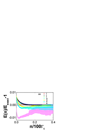
Figure 1: (Colors online) Comparison of exact ground state energy and the one obtained by LAQMC projection for the Hubbard with two holes ($N=16$) in the $18$ square lattice with $\Gamma_{t}=2.5U$. Notice the rapid convergence with projection time even for large $U/t$.

Release node technique: When there is sign problem, the Markov chain (Linearized Auxiliary fields Monte Carlo: efficient sampling of the fermion sign) is unstable because after a while half of the walkers will have negative sign and will cancel almost exactly the contribution of the ones with positive sign. In order to stabilize the process, we employ the standard release node technique introduced long time agoceperleyrelease , and adapted to the present case, to take into account only a ”discrete time” projection given by the power method. Therefore after the Markov chain equilibrates, we can have access with a single run and a very simple postprocessing, to all the history evolution of the energy as a function of the power method iterations starting from the very good estimate provided by the CPQMC state $\psi_{CPQMC}$, namely:

$$E_{n}={\langle\psi_{MF}|HG^{n}|\psi_{CPQMC}\rangle\over\langle\psi_{MF}|G^{n}|\psi_{CPQMC}\rangle}$$ (11)

for all $n\leq n_{\tau}$, where $n_{\tau}$ is the maximum release time allowed.

Guiding function: In order to define the appropriate guiding function $\psi_{g}$ at one electron per site filling $N=L$ we use an antiferromagnetic mean field Slater determinant with the order parameter along the x-spin axisbecca ; lugas .

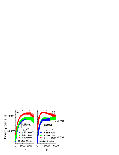
Figure 2: (Colors online) Energy as a function of the power method iterations using different mean field wave functions $\psi_{MF}$ for defining the guiding function in LAQMC. They differ for the value of the chemical potential $\mu_{0}$ and the BCS d-wave parameter $\Delta_{BCS}^{x^{2}-y^{2}}$ (see Ref.epaps, ). (a) $\mu_{0}=-0.198t$ (b) $\Delta_{BCS}^{x^{2}-y^{2}}=0.002t$

Moreover away from half-filling we use also a BCS like wave function with a small d-wave order parameter $\Delta_{BCS}^{x^{2}-y^{2}}$, when the ground state of the $U=0$ model is degenerate (open shell case). In the half-filled case $N=L$ in any bipartite lattice and for $U=0$, there is no sign problem (for $\Gamma_{t}$ large enough) and $\psi_{CPQMC}=\psi_{0}$. Therefore the method is exact already for $n=0$. On the contrary the TCL will lead to biased result without smearing the guiding function ($\epsilon=0$), due to lack of ergodicity in the Markov process. This is a well known problem in the standard CPQMCcpqmc , that can be definitively solved by means of the careful regularization introduced for $\epsilon>0$. As a particular example we show in Fig.(1) the comparison of the exact resultsbecca for the two hole case in the 18 site cluster. In this picture we reach convergence within statistical errors always with a small number of power iterations with no particular difficulty to sample the sign even for large $U/t$ values. From this picture we remark that only for very large $U/t$ ratios we observe that the convergence to the exact result is non monotonic as a function of $n$. In Fig. (2) the method is shown to work quite effectively as the CPQMC estimate remains very accurate also for a large cluster size, and convergence can be achieved much more quickly than the standard AFQMChlubina . In this figure we see that even when the initial wave function is not optimal it is possible to reach convergence with a quite good error bar. However it is also clear that a good initial guess allows a much more accurate energy estimate by using a much smaller $n_{\tau}$.

Finally we show the resultsepaps obtained for the energy per hole in Fig.(3), where $\delta=1-N/L$ is the hole concentration. If there is phase separation between an hole rich phase and the undoped insulator at $\delta=0$ the energy per hole should have a minimum at a critical doping $\delta_{c}$emery . Our reference energy at $\delta=0$ is exact and given by $E/L=-0.85996(5)t$ for $L\to\infty$ at $U/t=4$. For small doping, though we obtained a non monotonic behavior similar to the ones shown in Fig. 1 for $U/t>12t$, we were able to achieve convergence even in these particularly difficult cases using up to $n_{\tau}=10000$ power method iterations.

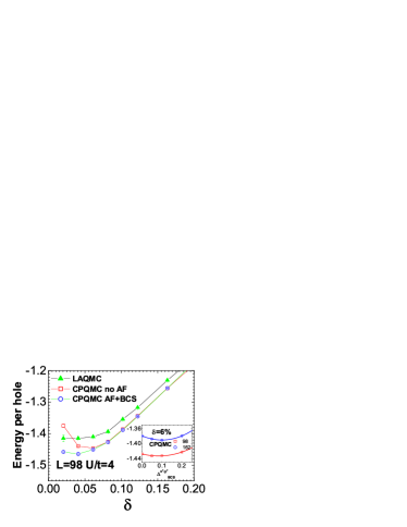
Figure 3: (Colors online) Energy per hole for LAQMC release nodes (full symbols) and CPQMC (empty symbols). Lines are guides to the eye.

Considering therefore our energy results for the larger possible cluster size, we find a clear flat region in the energy per hole $e_{h}(\delta)$, as shown in Fig.(3), that may suggest an incipient phase separationjarrell . This behavior is in disagreement with the standard CPQMC, where a clear minimum was found at doping $\delta_{c}\simeq 5\%$zhang for $L\simeq 100$. In order to understand this result, we have performed CPQMC calculations with our technique, and found, as clearly displayed in the same picture, that the CPQMC energy per hole is quite sensitive to the quality of the guiding function in the small doping region, and a magnetic guiding function containing both an antiferromagnetic and a d-wave order parameter greatly improves the CPQMC energy per hole, that becomes qualitatively similar to the LAQMC $e_{h}(\delta)$. Summirizing an infinite compressibility appears plausible only when the doping approaches zero, in contrast with the clearly bounded one obtained in the $t-J$ model with a similar guiding functionlugas . We believe that this difference is due to the particle-hole symmetry, that is not satisfied in the $t-J$ model, and instead could imply $e_{h}(\delta)\simeq\delta^{2}$ as in 1D.

In conclusion we have presented a new method for the simulation of the Hubbard model with about $100$ electrons, even when the sign problem prevents affordable calculations with standard techniques. Preliminary results show a very large but finite compressibility at small doping in the square lattice Hubbard model at $U/t=4$.

This work was supported by a PRACE grant 2010PA0447.

References

- (1) N. Trivedi and D. M. Ceperley Phys. Rev. B41, 4552 (1990).
- (2) S. Sorella and L. Capriotti Phys. Rev. B61, 2599 (2000).
- (3) J. E. Hirsch Phys. Rev. B31, 4403.
- (4) S.R. White et al Phys. Rev. B40, 506, (1989); S. Sorella et al. Europhys. Lett. 8, 663 (1989).
- (5) Philipp Werner et al. Phys. Rev. Lett. 97, 076405, (2006); N. V. Prokof’ev and B. V. Svistunov Phys. Rev. B77, 125101 (2008).
- (6) A. N. Rubtsov, V. V. Savkin, and A. I. Lichtenstein, Phys. Rev. B72, 035122 (2005).
- (7) S. Fahy and D.R. Hamann Phys. Rev. B43, 765 (1991).
- (8) S. Zhang, J. Carlson, and J.E. Gubernatis Phys. Rev. Lett. 78, 4486, (1997); J. Carlson et al., Phys. Rev. B59, 12788 (1999).
- (9) D. M. Ceperley, and B. J. Alder, Journal of Chemical Physics, 81, 5833 (1984).
- (10) C. Attaccalite and S. Sorella Phys. Rev. Lett. 100, 114501 (2008).
- (11) M. Calandra and S. Sorella, Phys. Rev. B57, 11446 (1998).
- (12) F. Becca, M. Capone and S. Sorella Phys. Rev. B62, 12700 (2000)
- (13) M. Lugas, L. Spanu, F. Becca, S. Sorella Phys. Rev. B74, 165122 (2006).
- (14) R. Hlubina , S. Sorella and F. Guinea, Phys. Rev. Lett. 78, 1343 (1997).
- (15) See Supplemental Material at [URL] for energy values and finite size scaling at .
- (16) V. J. Emery, S. A. Kivelson, and H. Q. Lin, Phys. Rev. Lett. 64, 475 (1990).
- (17) Chia-Chen Chang and Shiwei Zhang Phys. Rev. B 78, 165101 (2008).
- (18) E. Khatami et al. Phys. Rev. B81, 201101 (2010).