Abstract

We propose a quantitative method to estimate the statistical properties of sets of genes for which expression data are available and co-registered on a reference atlas of the brain. It is based on graph-theoretic properties of co-expression coefficients between pairs of genes. We apply this method to mouse genes from the Allen Gene Expression Atlas. Co-expression patterns of a list of several hundreds of genes related to addiction are analyzed, using ISH data produced for the mouse brain at the Allen Institute. It appears that large subsets of this set of genes are much more highly co-expressed than expected by chance.

Contents

1. 1 Introduction
2. 2 Model and gene-expression data
   1. 2.1 Data: the Allen Gene Expression Atlas (AGEA)
   2. 2.2 Co-expression matrices
   3. 2.3 Co-expression matrices as co-expression graphs
   4. 2.4 Thresholding a co-expression graph
   5. 2.5 Monte Carlo study
   6. 2.6 Empirical cumulative distribution functions of co-expression coefficients
      1. 2.6.1 Empirical distribution function
      2. 2.6.2 Bootstrapping: cumulative distribution functions of random sets of genes
3. 3 Application to a list of addiction-related genes
   1. 3.1 A set of 288 genes from NicSNP
   2. 3.2 Search for statistically significants subsets of fixed size

1 Introduction

In this era of complete genomes, genes are related to medical conditions by genome-wide association studies. This results in large lists of condition-related genes. It is desirable to prioritize some subsets of these lists for further study. High-throughput experiments have already provided neuroscience with a publicly-available dataset at a resultion of 200 microns for the mouse brain, the Allen Gene Expression Atlas (AGEA), [1, 2, 3, 4]. The AGEA can be used as a reference set to assess how exceptional a set of genes is. We define co-expression matrices for sets of genes, and study statistical properties of the underlying graphs by Monte Carlo methods.

These methods are applied to a set of 288 candidate genes extracted from the NicSNP database , http://zork.wustl.edu/nida/Results/data1.html, which have been linked to nicotine dependence, based on the statistical significance of allele frequency difference between cases and controls. These 288 genes are those for which mouse orthologs are found in the AGEA, with at least two datasets, one sagittal and one coronal.

The brainwide gene-expression data are used to compute co-expression networks. Restrictions to marker genes for brain regions defined by classical neuroanatomy [5, 6], or spatial clusters of gene-expression data [7, 8] could be used in order to work out the anatomical properties of co-expression, in order to interpret them in terms of connections [9, 10].

2 Model and gene-expression data

2.1 Data: the Allen Gene Expression Atlas (AGEA)

The Allen Gene Expression Atlas is a high-resolution, brain-wide dataset, that provides estimators of the number of mRNAs in the mouse brain at a resolution of 200 microns can be presented in the form of a voxel-by-gene matrix whose columns represent genes, and whose lines corresponds to voxels (emphi.e cubes of side 200 microns into which the brain is partitioned):

$$E(v,g)\simeq{\mathrm{Number\;of\;mRNAs\;for\;gene}}\;g\;{\mathrm{\;at\;voxel\;}}v.$$ (1)

The entries of the matrix $E$ are gene expression energies were obtained from the co-registration to a reference brain atlas of sets of ISH images of thousands of genes in the Allen Gene Expression Atlas [4]. For each of the genes, an eight-week old C57Bl/6J male mouse brain was prepared as unfixed, fresh-frozen tissue. The following steps were taken in an automatized pipeline :

• Colorimetric in situ hybridization;

• Automatic processing of the resulting images. In this step, tissue areas are found by eliminating artefacts, looking for cell-shaped objects of size $\simeq 10-30$ microns;
  

• Aggregation of the raw pixel data into a grid. The mouse brain is partitioned into $V=49,742$ cubic voxels of side 200 microns. All series of brain tissue are registered to a reference atlas [5]. For each voxel $v$, the expression energy of the gene $g$ is defined as a weighted sum of the greyscale-value intensities of pixels $p$ intersecting the voxel:

  $$E(v,g):=\frac{\sum_{p\in v}M(p)I(p)}{\sum_{p\in v}1},$$ (2)

  where $M(p)$ is a Boolean mask worked out by step 2 with value 1 if the pixel is expressing and 0 if it is non-expressing.
  

The present analysis is focused on genes for which sagittal and coronal data are available. We computed the correlation coefficients between sagittal and coronal data and selected the genes in the top-three quartiles of correlation ($G=3041$ genes), and used the coronal atlas .

2.2 Co-expression matrices

Since each gene in the AGEA has a gene-expression energy given by a positive number at each of the $V$ voxels, the columns of the matrix $E$ of gene-expression data are naturally identified to vectors in a $V$-dimensional space. This is a very high-dimensional space. However, given two genes, the two corresponding columns of the matrix $E$ span a two-dimensional vector-space. The simplest geometric quantity to study for this system of two vectors is the angle at which they intersect. As all the entries of the matrix $E$ are positive by construction, this angle is between 0 and $pi/2$. The angle between the two vectors is therefore completely characterized by its cosine, which is readily expressed in terms of the normalized columns of the matrix of gene-expression energies.

Consider the matrix $\tilde{E}$ of $L^{2}$-normalized columns of $E$:

$$\tilde{E}(v,g)=\frac{1}{\sqrt{\sum_{v=1}^{V}E(v,g)^{2}}}E(v,g).$$

The $g$-th columns of $\tilde{E}$ is the direction of the expression-vector of gene $g$ (the factor $\sqrt{\sum_{v=1}^{V}E(v,g)^{2}}$ is the Euclidean norm of the expression vector of gene $g$ in voxel space).

For any two genes $g$ and $g^{\prime}$, consider the following scalar product:

$${\mathrm{coExpr}}(g,g^{\prime})=\sum_{v=1}^{V}\tilde{E}(v,g)\tilde{E}(v,g^{\prime}).$$ (3)

This number is between 0 and 1 by construction. It is the cosine of the angle between the direction of the expression vectors of $g$ and $g^{\prime}$. We call it the co-expression, or cosine similarity, of genes $g$ and $g^{\prime}$. The more co-expressed $g$ and $g^{\prime}$ are in the brain, the closer their cosine similarity is to 1.

These numbers, which we computed for pairs of genes in the AGEA are naturally arranged in a matrix, denoted by $C^{\mathrm{atlas}}$, with the genes arranged in the same order as the list of genes in the AGEA:

$${C^{\mathrm{atlas}}}(g,g^{\prime})={\mathrm{coExpr}}(g,g^{\prime}).$$ (4)

This matrix is symmetric because the scalar product is. Its diagonal entries are all equal to one, as they correspond to the scalar product of normalized gene expression vectors with themselves. This diagonal is trivial in the sense that it expresses that the vector of expression energies of each gene in the atlas is perfectly aligned with itself. When we consider the distribution of the entries of the co-expression matrix, we really mean the distribution of the upper-diagonal coefficients.

2.3 Co-expression matrices as co-expression graphs

Given a set of genes curated from the literature, possibly studied using different methods, one may ask if these genes (or a subset) expression profiles across the brain are particularly close to each other. The study of the co-expression matrix is a quantitative way to assess how exceptional a set of genes is.

A set of strongly co-expressed genes corresponds to a submatrix of the co-expression matrix with large coefficients. In order to formalise this idea, we need to choose a way to define what a submatrix with large coefficients is. We propose to study the matrix in terms of the underlying graph, because this makes the results less dependent on the way genes are ordered. Even though considering the data as a matrix suggested the study of the angles between its column vectors, we are only interested in the set of co-expression between pairs of genes, and the set of pairs of genes does not depend on the order in which we present the genes of AGEA.

There are $G!$ ways of ordering the $G$ genes in the Allen Gene Expression Atlas. Generically they will generically give rise to different co-expression matrices, related by similarity transformation. But the sets of highly co-expressed genes are certainly invariant under these operations.

The co-expression matrix can be mapped to a weighted graph in a straightforward way (see Figure (1) for a toy-model with 9 genes). The vertices of the graph are the genes, and the edges are as follows:
- genes $g$ and $g^{\prime}$ are linked by an edge if their co-expression $C_{gg^{\prime}}$ is strictly positive.
- If an edge exists, it has weight $C_{gg^{\prime}}$.

Consider a set of genes of size $K$, for all of which data are available in the AGEA. They correspond to indices $(g_{1},\dots,g_{K})$ in the columns of the matrix $E$ of gene-expression data. We can construct a co-expression matrix just by extracting the coefficients of the co-expression matrix of the atlas corresponding to these genes. Let us denote this matrix $C^{\mathrm{set}}$:

$$C^{\mathrm{set}}=\left(C^{\mathrm{atlas}}(g,g^{\prime})\right)_{g,g^{\prime}\in\{g_{1},\dots,g_{K}\}}.$$ (5)

We would like to compare the properties of the matrix $C^{\mathrm{set}}$ to the ones of $C^{\mathrm{atlas}}$. Some quantities such as the average of the upper-diagonal coefficients can be readily computed for both matrices, there is a sample-size bias that prevents us from comparing the results directly. Instead, we are going to study some properties of the graph underlying $C^{\mathrm{set}}$, and to compare them to the properties of the graphs underlying submatrices of $C^{\mathrm{atlas}}$ of the same size.

2.4 Thresholding a co-expression graph

We have not formalized the notion of a large co-expression coefficients. It is most likely impossible to give a useful absolute definition of properties that would characterize large co-expression matrices, because the absolute values of co-expression depend a lot on the resolution and will not be reproduced in other atlases and/or datasets. For instance, in the limit of a very coarse resolution, the data will not reflect much of the microscopic details of the gene-expression profiles, and the entries of the co-expression matrix will be larger on average than in the present atlas. In the limit of a very fine resolution, for instance if one took the Allen data at full (one micron) resolution, the shape of the soma would become visible, and the expression is zero outside the soma. Even after co-registration of all the ISH image series to the Reference Atlas, the spatial distribution of somas would vary from brain to brain and the co-expression coefficients would therefore be much lower on average that at a resolution of 200 microns.

Hence we have to define large co-expression matrices in relative terms, using thresholds on the value of co-expression that describe the whole set of possible values. The coefficients of the co-expression networks are numbers between $0$ and $1$ by construction. We define the following thresholding procedure on co-expression graphs: given a threshold $\rho$ between $0$ and $1$, and a co-expression matrix denoted by $C$ (which can come from any set of genes in the AGEA), put to zero all the coefficients that are lower than this coefficient. This graph comes from a thresholded co-expression matrix $C_{\rho}$ such that the underlying graph has only edges with weight larger than the threshold:

$$C_{\rho}(i,j)=C(i,j)\times\mathbf{1}(C(i,j)\geq\rho).$$ (6)

By construction we have $C_{0}=C$. The graph corresponding to the matrix $C_{\rho}$ has connected components, and each connected component has a certain number of genes in it. Our notion of a large co-expression matrix, relative to a threshold $\rho$ is therefore a topological property of the graph (see Figure 1 for an illustration of a toy-model with only 10 genes) underlying the thresholded matrix $C_{\rho}$.

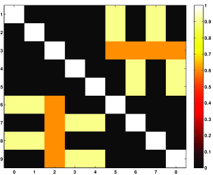
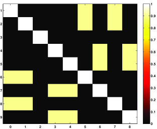
Figure 1: A toy model with 9 genes, and only three distinct values of co-expression, 0, 0.6 and 0.9, for simplicity. The two heat maps of the co-expression matrix correspond to two different orderings of the genes, but the co-expression coefficients are the same. On the second heat map, it is obvious by eye that the first four genes form an ’island’ with high co-expression, but it is hard to observe this on the first map, simply because these genes are not placed at adjacent columns. However, plots of the underlying graph show that these genes stay connected even when the links with strength weaker than a threshold are pruned.

If the initial co-expression matrix $C$ has size $G$ (i.e. corresponds to $g$ genes), then for every integer $k$ between 1 and $G$ we can count the number $N_{\rho}(k)$ of connected components of $C_{\rho}$ that have exactly $k$ genes in them.

We can study the average size of connected components of thresholded co-expression networks

$$\mathcal{G}(\rho)=\frac{\sum_{k=1}^{G}kN_{\rho}(k)}{\sum_{k=1}^{G}N_{\rho}(k)},$$ (7)

and the size of the largest connected component:

$$\mathcal{A}(\rho)=\frac{\sum_{k=1}^{G}kN_{\rho}(k)}{\sum_{k=1}^{G}N_{\rho}(k)},$$ (8)

$$\mathcal{M}(\rho)=\mathrm{max}\left\{k\in[1..G],N_{\rho}(k)>0\right\},$$ (9)

as a function of the threshold $\rho$. We can see that $\mathcal{A}(0)$ is the size of the set of genes, as the whole set is connected. At large thresholds every single singe is disconnected from the other genes, as having co-expression equal to one is equivalent to having exactly the same expression across the whole brain. So at threshold 1 all the connected components have size one, and $\mathcal{G}(1)=1$. Examples are given below for several values of $G$.

2.5 Monte Carlo study

In order to eliminate the sample-size bias we have to compare graph properties of $C^{\mathrm{set}}$ to the graph properties of matrice sof the same size, drawn from $C^{\mathrm{atlas}}$. If $C^{\mathrm{set}}$ has size $K$, we can repeatedly draw random sets of genes of size $K$, extract the corresponding submatrices of the full co-expression matrix $C^{\mathrm{atlas}}$, and compute the size of the largest connected component for each value of the threshold for which $C^{\mathrm{set}}$ was studied.

In order to explore the space of thresholds we have to choose a discrete set of threshold regularly spaced between 0 and 1. Call $R$ the number of random draws. The computations can be described as follows in pseudocode:
1. Choose a number of thresholds $T$ to study.
2. Choose a number of draws $R$ to be performed for each value
of the threshold.
3. For each integer $t$ between $1$ and $T$:
3.a. consider the threshold $\rho_{t}=\frac{t}{T};$
3.b. compute the connected components of the thresholded matrix $C^{\mathrm{set}}_{\rho_{t}}$;
call $\mathcal{M}^{\mathrm{set}}(\rho)$ the size of the largest connected component;
4. for each integer $r$ between $1$ and $R$:
draw a random set of distinct indices of size $K$ from [1..G],
extract the corresponding submatrix of $C^{\mathrm{atlas}}$;
call it $C^{r}$, and repeat step 3 after substituting $C^{r}$ to $C^{set}$;
call $\mathcal{M}^{\mathrm{r}}(\rho_{t})$ the size of the largest connected component of $C^{\mathrm{r}}_{\rho_{t}}$. The two values chosen in the first step are obviously dictated by the speed on the computation. The number of mathematical operation is $O(TR)$. If interesting and/or regular behaviour is observed around a particular threshold, the algorithm can be rerun on a set of threshold centered around these values, because the results of loops associated to different values of the threshold are independent.

At each value $\rho$ of the threshold, we therefore have:
- the size of the maximal connected component $\mathcal{M}^{\mathrm{set}}(\rho)$,
- a distribution of $R$ numbers, each of wchich is the size of the largest connected components of a random submatrix of the same size as the set of genes to study, thresholded at $\rho$.
We can study where in $\mathcal{M}^{\mathrm{set}}(\rho)$ sits in the distribution by computing the number of standard deviations by which it deviates from the mean across all draws:

$$\mu(\rho)=\frac{1}{R}\sum_{r=1}^{R}\mathcal{M}^{\mathrm{r}}(\rho),$$

$$\sigma(\rho):=\sqrt{\frac{1}{R}\sum_{r=1}^{R}(\mathcal{M}^{\mathrm{r}}(\rho)-\mu(\rho))^{2}},$$

$$\delta(\rho):=\frac{\mathcal{M}^{\mathrm{set}}(\rho)}{\sigma(\rho)}$$

2.6 Empirical cumulative distribution functions of co-expression coefficients

2.6.1 Empirical distribution function

In order to complement the graph-theoretic approach, we can study the cumulative distribution function of the co-expression coefficients in the special set, and compare it to the one resulting from randonm sets of genes of the same size.

Let us plot the empirical distribution functions of the coefficients above the diagonal in the co-expression matrices $C$, for $C=C^{\mathrm{atlas}}$ in blue, for $C=C^{\mathrm{set}}$ in red. These distribution functions are evaluated in the following way: Let $N$ denote the size of the matrix $C$, i.e. the number of genes from which $C$ was computed. Consider the coefficients above the diagonal (which are the meaningful quantities in $C$ by construction) and arrange them into a vector $C_{\mathrm{vec}}$ with $N^{\prime}=N(N-1)/2$ components: $C_{{\mathrm{vec}}}=\{C_{gh}\}_{1\leq g\leq N,h>g}$. The components are numbers between 0 and 1. For every number between 0 and 1, the empirical distribution function of $C$, denoted by ${\mathrm{edf}}^{C}$ is defined as the fraction of the components of $C_{{\mathrm{vec}}}$ that are smaller than this number:

$${\mathrm{edf}}^{C}:[0,1]\rightarrow[0,1]$$

$$x\mapsto\frac{1}{N^{\prime}}\sum_{k=1}^{N^{\prime}}\delta_{C_{{\mathrm{vec}}}(k)\leq x}.$$

2.6.2 Bootstrapping: cumulative distribution functions of random sets of genes

We would like to compare the network of interest to random networks of the same size, drawn from the set of genes in our dataset. The procedure is exactly the same as with the thresholded matrices, except that the quantities computed from the random draws are cumulative dictribution functions rather than connected components. Let us repeteadly draw random subsets of genes with the same number of elements as the set of interest, compute the empirical distribution function of the corresponding submatrix of $C^{\mathcal{T}}$ and average over the draws. The average over the draws should converge towards the one of a typical network of $N$ genes, when the number of draws becomes larger.

3 Application to a list of addiction-related genes

3.1 A set of 288 genes from NicSNP

We applied the graph-theoretic method described above to a set of 288 genes related to nicotine addiction gathered from the NicSNP database [11]. The results are presented on Figure (2). The special set of 288 genes is not more co-expressed than expected by chance, since thresholding at high values of the co-expression coefficient induces connected components that are smaller on average than those of random sets of genes of size 288.

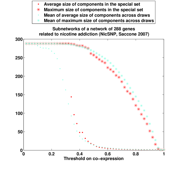
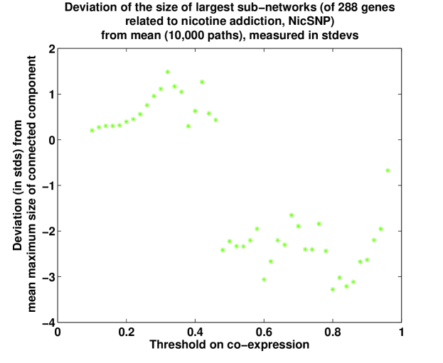
Figure 2: Statistics of maximum and average size of connected components of thresholded co-expression graphs (addiction-related genes in red, random sets in cyan), 288 genes.

The result is therefore rather negative : there is no clear statistical significance of the connected component of the co-expression matrix of these genes, especially at the highest levels of co-expression. The use of the proposed graph-theoretic method is however adapted to the determination of exceptional sets of genes that are small in scale of a pre-determined set of condition-related genes.

The study of the cumulative distribution function of co-expression for the full set of 288 genes is also rather negative (see Figure 3), as the cdf grows faster than expected by chance for small values of the co-expression.

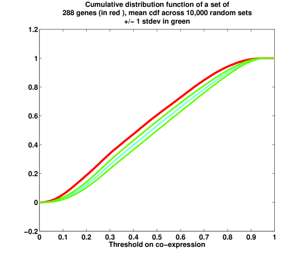
Figure 3: Cumulative distribution function of cosine similarities in co-expression graphs of 288 genes related to nictine addiction.

3.2 Search for statistically significants subsets of fixed size

It may be the case that subsets of the list of genes to study exhibit exceptional co-expression properties, while the whole set is not particularly co-expressed. In order to prioritize subsets of the genes in NicSNP for further study, we would like to identify such subsets.

We would be in that case for instance if the first few genes had all very-high co-expression with each other, while the next genes are orthogonal to them as well as with each other , corresponding to a co-expression matrix with a square of high coefficients (of size, say, $G_{high}$) in the upper-left corner, and zeros everywhere. However, the order in which genes are presented does not ensure that the set of highly expressed genes should be the set of the first $G_{high}$ genes.

In order to detect such subsets of genes, one can allow the user to specify a list $I_{init}$ few indices in the list of genes, that have been observed to have high co-expression, or that are of special interest as a subset.

For a thorough search of exceptional sets of co-expressed genes of a given size, one can take the list $I^{init}$ to consist of just one index, and repeat the procedure for all posible choice of this index.

Let the list $I^{init}$ consist of $G_{init}$ indices:

$$I^{init}=:(i_{1},\dots,i_{G_{high}}).$$

One can grow it one element at a time by adding to it the gene that co-expresses the most on average with the genes that are already in the list. That is, for each gene whose index is not in $I^{init}$, compute the sums of co-expressions with genes whose index is in $I^{init}$, and pick the index $g_{suppl}$ that maximizes the sum:

$$c^{extra}:=\left(\sum_{j\in I^{init}}C^{small}_{ij}\right)_{i\notin I_{init}}.$$

$$g_{suppl}:={\mathrm{argmax}}_{i\notin I^{init}}\left(c^{extra}_{i}\right).$$

The gene with index $g_{suppl}$ is then added to the list:

$$I^{init}\rightarrow[I^{init},g_{suppl}],$$

and the co-expression matrix corresponding to the new list can be studied by the thresholding technique described above.

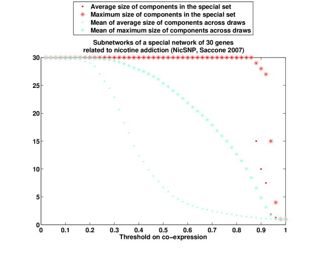
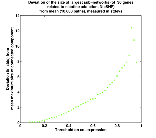
Figure 4: Statistics of maximum and average size of connected components of thresholded co-expression graphs (addiction-related genes in red, random sets in cyan), 30 genes.

This procedure was used to construct a set of 30 genes, which was studied using the graph-theoretic procedure. The names of these genes are the following: Gprasp1, Uchl1, Grin1, Ctsb, Gria2, Phyh, Snap25, Actr2, Gabarapl1, Calm1, Dlgh4, Syt1, Ppp1r9b, Cttn, Grik5, Gria3, Slc1a2, Ssbp4, Gria4, Hint1, Atrx, Per1, Slc1a1, Gabbr2, Chrm1, Gtpbp9, Cap1, Fbxw2, Mtch2, Socs5.

The results are shown of Figure (4), from which it is quite clear that this set of genes is exceptionally co-expressed. The procedure can then be repeated on the set of 258 nicotine-related genes obtained by removing those genes.

The study of the cumulative distribution function of co-expression for this special set of 30 genes deviates (see Figure 5), as the cdf takes off at higher values of the co-expression than expected by chance.

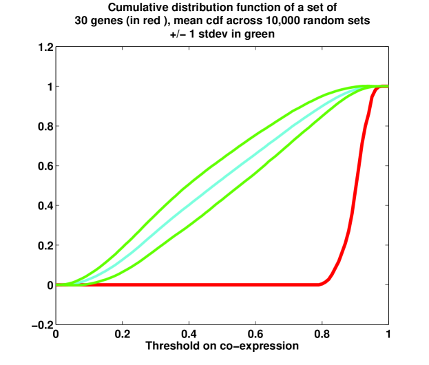
Figure 5: Cumulative distribution function of cosine similarities in co-expression graphs of 30 genes related to nicotine addiction (in red).

References

- 1. E.S. Lein et al., Genome-wide atlas of gene expression in the adult mouse brain, Nature 445 (2007), 168–176.
- 2. L. Ng, M. Hawrylycz, and D. Haynor (2005), Automated high-throughput registration for localizing 3D mouse brain gene expression using ITK, Insight-Journal (2005).
- 3. L. Ng et al., Neuroinformatics for Genome-Wide 3-D Gene Expression Mapping in the Mouse Brain, IEEE/ACM Transactions on Computational Biology and Bioinformatics (2007), 382–393.
- 4. L. Ng, A. Bernard, C. Lau, C.C. Overly, H.-W. Dong, C. Kuan, S. Pathak, S.M. Sunkin, C. Dang, J.W. Bohland, H. Bokil, P.P. Mitra, L. Puelles, J. Hohmann, D.J. Anderson, E.S. Lein, A.R. Jones and M. Hawrylycz, An anatomic gene expression atlas of the adult mouse brain, Nature Neuroscience 12, 356–362 (2009).
- 5. H.-W. Dong, The Allen reference atlas: a digital brain atlas of the C57BL/6J male mouse, Wiley, 2007.
- 6. P. Grange and P.P. Mitra, Determination of optimal sets of genes as markers of anatomical regions in the mouse brain, [arXiv:1105.1217 [q-bio.QM]].
- 7. T. Hastie, R. Tibshirani, J. Friedman (2009), The elements of statistical learning: data mining, inference, and prediction, Springer Series in Statistics.
- 8. Bohland JW, Bokil H, Pathak SD, Lee CK, Ng L et al. (2010),Clustering of spatial gene expression patterns in the mouse brain and comparison with classical neuroanatomy, Methods.
- 9. J.W. Bohland et al. (2009), A proposal for a coordinated effort for the determination of brainwide neuroanatomical connectivity in model organisms at a mesoscopic scale, PLoS Computational Biology, 5(3), e1000334. PMID: 19325892.
- 10. P. Grange and P.P. Mitra, Algorithmic choice of coordinates for injections into the brain: encoding a neuroanatomical atlas on a grid, arXiv:1104.2616.
- 11. S.F. Saccone, N.L. Saccone, G.E. Swan, P.A.F. Madden, A.M. Goate, J.P. Rice and L.J. Bierut, Systematic biological prioritization after a genome-wide association study: an application to nicotine dependence, Bioinformatics (2008), 24, 1805–1811.