Electronic standing waves on the surface of the topological insulator Bi₂Te₃

Abstract

A line defect on a metallic surface induces standing waves in the electronic local density of states (LDOS). Asymptotically far from the defect, the wave number of the LDOS oscillations at the Fermi energy is usually equal to the distance between nesting segments of the Fermi contour, and the envelope of the LDOS oscillations shows a power-law decay as moving away from the line defect. Here, we theoretically analyze the LDOS oscillations close to a line defect on the surface of the topological insulator Bi₂Te₃, and identify an important preasymptotic contribution with wave-number and decay characteristics markedly different from the asymptotic contributions. The calculated energy dependence of the wave number of the preasymptotic LDOS oscillations is in quantitative agreement with the result of a recent scanning tunneling microscopy experiment [Phys. Rev. Lett. 104, 016401 (2010)].

I Introduction

Distinct surface-electronic properties, potentially relevant for spintronic applications, arise from the strong spin-orbit interaction in three-dimensional topological insulators (3DTIs) Hasan-review . Although the bulk electronic structure of these materials resembles that of standard band insulators with electronic bands separated by an energy gap, the valence and conduction bands of the surface states form a conical dispersion and touch at the center of the surface Brillouin zone. These gapless surface states lack the standard twofold spin degeneracy, they are protected against backscattering, and the spin orientation of each plane-wave surface state is determined unambiguously by its momentum vector.

In the past few years, surface-sensitive experimental techniques have been utilized to explore the remarkable properties of the surface electrons in 3DTIs. The linear, Dirac-cone-like electronic dispersion and deviations from that were observed in various 3DTI materials using angle-resolved photoemission spectroscopy Hsieh-nature ; Hsieh-science ; Xia-naturephysics ; Chen-Bi2Te3 ; BiSexp ; Hsieh-prl (ARPES), and the correlation between spin and momentum was demonstrated by the spin-resolved version of the same technique Hsieh-science . The role of electron scattering off pointlike impurities and line defects on 3DTI surfaces, highly relevant for future attempts to design electronic devices based on these materials, has been studied via scanning tunneling microscopy (STM) Roushan-nature ; TongZhang-edgeimpurity ; BiTexp ; JungpilSeo-antimony ; JingWang . In the vicinity of obstacles on the surface, characteristic standing wave patterns are formed due to the interference of initial and final scattering states 2DEG . These electronic standing waves contribute to the local density of states (local DOS, LDOS), therefore real-space mapping of them is possible via STM. Theories describing the standing waves on 3DTI surfaces have also been formulated recently FuHam ; WeiChengLee-prb-bite ; LDOS_Zhou ; Guo-ftstm ; QiangHuaWang-ldos ; LDOS_Biswas ; Biswas_arxiv ; Liu-arxiv .

A line defect has translational symmetry in the direction it stretches along, hence the electronic standing waves in its vicinity are essentially one-dimensional (1D), (i.e., the LDOS varies only along the axis perpendicular to the line defect). This simple 1D character of the induced LDOS pattern implies a relatively straightforward experimental and theoretical analysis of the effect, which serves as a strong motivation to consider such arrangements. A line defect arises naturally at the edge of a step formed by an extra crystal layer on the surface, 2DEG ; BiTexp ; TongZhang-edgeimpurity ; JingWang hence this 1D setup is accessible experimentally.

Information on the electronic system can be extracted from the asymptotic decay exponent and wave number of LDOS oscillation around line defects. Theoretical results LDOS_Zhou ; LDOS_Biswas ; Biswas_arxiv ; JingWang indicate that the LDOS oscillations on the surface of a 3DTI, asymptotically far from a line defect and within the energy range of linear dispersion, decay with the distance $x$ from the defect as $x^{-3/2}$. This decay exponent is in contrast with the $\sim x^{-1/2}$ decay seen in a standard two-dimensional electron gas, 2DEG and arises as a consequence of the absence of backscattering characteristic of surface electrons in 3DTIs. Recent STM data agrees with this prediction. JingWang The wave vector of the asymptotic LDOS oscillations is usually equal to the distance between nesting segments of the constant-energy contour (CEC), which is the diameter of the Fermi circle in the above-mentioned case. This has been used in a recent experiment TongZhang-edgeimpurity to confirm the linear dispersion and to infer the Fermi velocity on the Dirac cone in Bi₂Te₃.

For energies well above the Dirac point, the topological surface conduction band of Bi₂Te₃  is subject to strong hexagonal warping. STM data corresponding to this energy range is available BiTexp ; JingWang , however, the rather complex geometry of the dispersion relation has so far prevented an unambiguous theoretical interpretation of the observations. In this work, we provide a theoretical investigation of LDOS oscillations created by a line defect on the surface of Bi₂Te₃. We describe the effect in an exact scattering-theory framework LDOS_Zhou , yielding results that are not restricted to the spatial region asymptotically far from the defect, but hold also in the vicinity thereof. This enables us to directly compare our results with experimental data, the latter being usually taken close to the defect where features of the LDOS are most pronounced. In the energy range of strong hexagonal warping, we identify a significant pre-asymptotic contribution to the LDOS oscillations, with wave number quantitatively matching that of a recent experiment BiTexp .

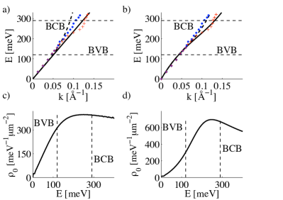
Figure 1: (a,b) Surface-state conduction-band dispersion of Bi₂Te₃ along the $\Gamma M$ (solid line) and $\Gamma K$ (dashed line) directions of the surface Brillouin zone. (c,d) Surface-state conduction-band density of states of Bi₂Te₃. For (a) and (c), Eq. (2) was used with parameter valuesFuHam $v_{0}=2.55$ eVÅ, $\lambda=250$ eVų and $\alpha,\gamma=0$. For (b) and (d), the parameter values $v_{0}=3.5\;{\rm eV\AA}$, $\lambda=150\;{\rm eV\AA^{3}}$, $\alpha=21\;{\rm\AA^{2}}$ and $\gamma=-19.5\;{\rm eV\AA^{2}}$ were used. Red crosses (blue points) represent the measured dispersion along $\Gamma M$ ($\Gamma K$) (data taken from Ref. BiTexp, ). The zero of energy corresponds to the Dirac point of the spectrum. Energy intervals overlapping with the bulk valence band (BVB) and bulk conduction band (BCB) are also shown.

II Band-structure parameters.

In order to base our forthcoming calculations on an accurate surface-band dispersion, we first establish accurate values of the relevant band-structure parameters (defined below) of Bi₂Te₃. ARPES measurements BiTexp indicate that the surface bands of 3DTIs with the crystal structure of Bi₂Te₃ are subject to hexagonal warping, which can be described by the envelope-function Hamiltonian FuHam :

$$H(\mathbf{k})=\gamma\mathbf{k}^{2}+v_{\mathbf{k}}\left(k_{x}\sigma_{y}-k_{y}\sigma_{x}\right)+\frac{i\lambda}{2}\left(k_{+}^{3}-k_{-}^{3}\right)\sigma_{z}\;,$$ (1)

where $v_{\mathbf{k}}=v_{0}(1+\alpha\mathbf{k}^{2})$, and $k_{\pm}=k_{x}\pm ik_{y}$. Here, $(\sigma_{x},\sigma_{y},\sigma_{z})$ is the vector of Pauli matrices representing spin, $v_{0},\lambda,\gamma$ and $\alpha$ are band-structure parameters, $\mathbf{k}=(k_{x},k_{y})$, and $k_{x}$ and $k_{y}$ are momentum components along the $\Gamma M$ and $\Gamma K$ directions of the surface Brillouin zone, respectively. For convenience, we performed a $+\pi/2$ rotation around the $z$ axis compared to the Hamiltonian in Ref. FuHam, . Energy eigenvalues of $H$ in Eq. (1) are

$$\varepsilon_{\pm}(\mathbf{k})=\gamma\mathbf{k}^{2}\pm\sqrt{\left(v_{\mathbf{k}}\mathbf{k}\right)^{2}+\lambda^{2}k_{y}^{2}(k_{y}^{2}-3k_{x}^{2})^{2}}\;,$$ (2)

where $+$ ($-$) stands for conduction (valence) band. Higher-order termsBasak-prb-spintexture in $\bf k$ can also be included in $H$ .

Satisfactory agreement between the spectrum in Eq. (2) and the ARPES spectra of Bi₂Se₃ surface states BiSexp can be obtained by neglecting the band-structure parameters $\gamma$ and $\alpha$. In Bi₂Te₃ however, the conduction-band dispersion measured along the $\Gamma M$ direction, shown with red crosses in Figs. 1a,b, has a sub-linear segment, which can be theoretically reproduced by Eq. (2) only if $\gamma$ and $\alpha$ are finite. We find that using the band-structure parameter set $v_{0}=3.5\;{\rm eV\AA}$, $\lambda=150\;{\rm eV\AA^{3}}$, $\alpha=21\;{\rm\AA^{2}}$ and $\gamma=-19.5\;{\rm eV\AA^{2}}$, the measured dispersion relations along the $\Gamma K$ and $\Gamma M$ directions and the surface density of states (Fig. 1c,d of Ref. BiTexp, ) are accurately described by $H$ [Eq. (1)] up to 335 meV above the Dirac point. We use these parameter values throughout this paper. Fig. 1a and 1b (Fig. 1c and 1d) compares the theoretical surface-state dispersion (density of states) calculated with a parameter set used in an earlier workFuHam , and the above parameter set that we found to be optimal, respectively. Further considerations used to find the optimal parameter set above are included in Appendix A.

III Model.

Our goal is to theoretically describe the oscillations in the surface-state conduction-band LDOS induced by a line defect, e.g., the edge of an atomic terrace 2DEG ; TongZhang-edgeimpurity ; JungpilSeo-antimony ; BiTexp ; JingWang , on the surface of Bi₂Te₃. For the moment we assume that the defect forms a straight line that coincides with the $y$ axis (see Fig. 2). Following Ref. LDOS_Zhou, , we model the system with the Hamiltonian $H+V$, where effect of the defect is described via the potential $V(x)=V_{0}\Theta(-x)$.

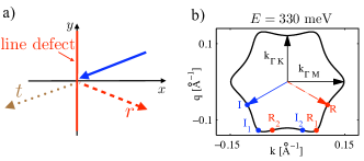
Figure 2: (a) An incident wave from the $x>0$ region (solid arrow) is partially reflected (dashed arrow) and transmitted (dotted arrow) at a line defect, e.g., an atomic terrace, on the surface of Bi₂Te₃. (b) Hexagonally warped constant-energy contour in reciprocal space, corresponding to energy $E=330$ meV above the Dirac point. Incident and reflected wave vectors from (a) are also shown.

Our analysis of the LDOS oscillations is based on exact energy eigenstates describing scattering of conduction-band electrons by the line defect (see Fig. 2). Therefore we first describe the scattering process of a plane wave energy eigenstate $\Phi_{k,q}(x,y)e^{iqy}=e^{iqy}e^{ikx}\chi_{k,q}$ incident from, say, the $x>0$ side of the edge, with momentum components $k\equiv k_{x}$ and $q\equiv k_{y}$, energy $E$, and spin wave function $\chi_{k,q}$. Scattering at the line defect is elastic, hence the energy $E$ is conserved. The momentum component $q$ parallel to the defect is also conserved due to translational invariance in the $y$ direction. The value of $q$ determines the number of propagating waves at a given energy. For example, in Fig. 2b, the number of propagating waves can be two (I and R) or four (I₁, I₂, R₁, R₂), depending on $q$.

However, the incident plane wave can be scattered into coherent superpositions of three reflected and three transmitted partial waves, for the following reasons. On the $x>0$ side of the defect, the equation $E=\varepsilon_{+}(k_{r},q)$ has six complex solutions $k_{r,1},\dots k_{r,6}$ for given values of $E$ and $q$, which follows from Eq. (2) (the numerical method used to obtain these solutions is described in Appendix B). Three of the $k_{r,p}$-s correspond to propagating waves moving away from the defect or evanescent modes. The associated wave functions $\Phi_{k_{r,p},q}=e^{iqy}e^{ik_{r,p}x}\chi(k_{r,p},q)$ ($p=1,2,3$) should be included in the Ansatz of the complete scattering state. The remaining three solutions $k_{r,p}$ $(p=4,5,6)$ correspond to propagating waves towards the defect or diverging modes, hence they are disregarded.

These arguments, together with their generalization to transmitted waves, imply that the $x$-dependent component of the complete scattering wave function is

$$\psi^{(R)}_{k,q}(x)=\left\{\begin{array}[]{cc}\Phi_{k,q}(x)+\sum\limits_{p=1}^{3}r_{kq,p}\alpha_{kq,p}\Phi_{k_{r,p},q}(x)&\textrm{if }x>0\;,\\ \sum\limits_{p=1}^{3}t_{kq,p}\beta_{kq,p}\Phi_{k_{t,p},q}(x)&\textrm{if }x<0\;,\end{array}\right.$$ (5)

where

$$\alpha_{kq,p} = \left\{\begin{array}[]{ll}\sqrt{\frac{|v_{\perp,k,q}|}{|v_{\perp,k_{r,p},q}|}}&\textrm{if }k_{r,p}\in\mathbb{R},\\ 1&\textrm{otherwise},\end{array}\right.$$ (8)

$$\beta_{kq,p} = \left\{\begin{array}[]{ll}\sqrt{\frac{|v_{\perp,k,q}|}{|v_{\perp,k_{t,p},q}|}}&\textrm{if }k_{t,p}\in\mathbb{R},\\ 1&\textrm{otherwise}.\end{array}\right.$$ (11)

Here, the $r$-s and $t$-s are reflection and transmission coefficients, $v_{\perp,k,q}$ is the $x$-component of the group velocity of the plane wave with wave-vector components $(k,q)$, and the factors $\alpha$ and $\beta$ ensure the unitarity of the scattering matrix built up from the reflection and transmission coefficients. Evanescent modes are not subject to the unitarity requirement, hence we are allowed to make the above arbitrary choice $\alpha=\beta=1$ for partial waves with complex wave vectors. As the Hamiltonian is a third-order differential operator, partial waves at the two sides of the defect should be matched via boundary conditions ensuring their continuity as well as the continuity of their first and second derivatives. The scattering state $\psi_{k,q}^{(L)}$ of a plane wave incident from the left side ($x<0$) of the defect can be described analogously.

The LDOS at a given energy $E$ and position $x$ is expressed with the exact scattering states as

$$\rho(E,x)=\frac{1}{(2\pi)^{2}\hbar}\sum_{d=L,R}\int_{\Gamma_{E}^{(d)}}d\kappa\frac{|\psi_{k,q}^{(d)}(x)|^{2}}{v(k,q)},$$ (12)

where $\Gamma_{E}^{(R)}$ [$\Gamma_{E}^{(L)}$] is the wave-vector contour of waves that (i) are incident from the right [left] side of the line defect, and (ii) have energy $E$. Note that $\Gamma_{E}^{(d)}$ breaks up to disconnected pieces for strong hexagonal warping, e.g., in Fig. 2b, the points $I_{1}$ and $I_{2}$ belong to $\Gamma_{E}^{(R)}$ but $R_{1}$ and $R_{2}$ do not. (The wave-vector contour $\Gamma_{E}^{(R)}$ is shown in Fig. 3b, there it is formed as the union of the thick blue lines.) The infinitesimal line segment along $\Gamma_{E}^{(L,R)}$ is denoted by $d\kappa$, and $v(k,q)$ is magnitude of the group velocity of the wave with momentum vector $(k,q)$. Using the exact scattering wave functions $\psi^{(d)}_{k,q}$, we evaluate the integral in Eq. (12) numerically. To account for the inevitable roughness of the line defect and to suppress noise due to the limited precision of the numerical integration, we average the LDOS oscillations $\delta\rho(x)$ over the angular range $[-5^{\circ},5^{\circ}]$ of the line defect orientation with respect to the $\Gamma K$ direction.

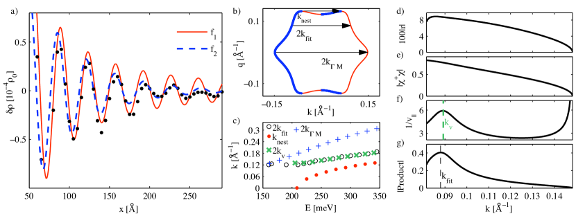
Figure 3: (a) Position-dependent contribution $\delta\rho(E,x)$ (solid line) to the LDOS at energy $E=330$ meV in the vicinity of a line defect (black points). Red solid and blue dashed lines are fits of the functions $f_{1}$ and $f_{2}$ (see text), respectively, to the data. $\rho_{0}=628\ {\rm meV}^{-1}\mu{\rm m}^{-2}$. (b) Constant-energy contour at the same energy, and relevant scattering wave vectors in reciprocal space. Thick blue (thin red) pieces of the contour correspond to left-moving (right-moving) plane waves. The union of the thick blue pieces form $\Gamma_{E}^{(R)}$ in Eq. (12). (c) Dominant wave number $2k_{\rm fit}$ of $\delta\rho(E,x)$ (open circles), and characteristic wave numbers $k_{\rm nest}$ (red points), $k_{\rm v}$ (green diagonal crosses) and $2k_{\Gamma{\rm M}}$ (blue crosses) of the constant-energy contour, as functions of energy $E$. (d) Magnitude of reflection amplitude $|r|\equiv|r_{k,q^{\prime}}|$, (e) magnitude of spinor overlap $|\chi^{\dagger}\chi|\equiv|\chi_{k,q^{\prime}}^{\dagger}\chi_{-k,q^{\prime}}|$, (f) magnitude of the inverse of the parallel-to-defect group velocity component $v_{\parallel}(k)$ (in units of $10^{-6}\,{\rm s}/{\rm m}$), and (g) the product of the above three quantitites (in units of $10^{-6}\,{\rm s}/{\rm m}$), as functions of perpendicular-to-defect wave number component $k$.

IV Results.

In Fig. 3a, we plot the numerically computed LDOS oscillations $\delta\rho(x)\equiv\rho(x)-\rho_{0}$ (black points) on the $x>0$ side of the defect, corresponding to energy $E=330$ meV and potential step height $V_{0}=-150$ meV. Recent theories using asymptotic analysis JingWang ; Biswas_arxiv suggest that the LDOS oscillations in the vicinity of a line defect on the surface of Bi₂Te₃ decay no faster than $x^{-3/2}$. Motivated by this finding, we fit the function $f_{1}(x)=A_{1}\sin(2k_{1}x+\varphi_{1})x^{-3/2}$ via fitting parameters $A_{1}$, $k_{1}$, and $\varphi_{1}$ to the results (shown as red solid line). We also fit an exponentially decaying function $f_{2}(x)=A_{2}\sin(2k_{\rm fit}x+\varphi_{2})e^{-x/L}$ via fitting parameters $A_{2}$, $k_{\rm fit}$, $\varphi_{2}$ and $L$ (blue dashed line). The two major features of our numerical result $\delta\rho(x)$ are as follows. (i) Comparison of the three curves suggests that the decay of $\delta\rho(x)$ is better described by the exponentially decaying function $f_{2}(x)$ than by $f_{1}(x)$ having power-law decay (see Appendix C for further details). (ii) The wave-number value obtained from fitting $f_{2}(x)$ is $2k_{\rm fit}\approx 0.178$ Å^-1.

Expectations for the wave number of the LDOS oscillations can be drawn from asymptotic analysis JingWang ; Biswas_arxiv . That suggests that the wave number of an electronic standing wave at a given energy $E$ is associated to wave vectors connecting nesting segments of the corresponding CEC 2DEG ; FuHam ; Biswas_arxiv , i.e., $2k_{\Gamma M}=0.297$ Å^-1 or $k_{\rm nest}=0.126$ Å^-1 depicted in Fig. 3b. As the wave number $2k_{\rm fit}$ characteristic of our data $\delta\rho(x)$ deviates significantly from $2k_{\Gamma M}$ and $k_{\rm nest}$, and its decay is exponential rather than power-law, we conclude that $\delta\rho(x)$ is dominated by a pre-asymptotic contribution in the considered spatial range.

In what follows, we argue that (i) the pre-asymptotic component of the LDOS is due to the interference of incoming and reflected partial waves, i.e., the role of evanescent and transmitted partial waves is negligible, and (ii) the appearance of the characteristic wave number $2k_{\rm fit}$ in the LDOS oscillations is due to the non-monotonic behavior of the parallel-to-defect group velocity component along the CEC. To this end, we now consider only the interference contribution of incoming and reflected propagating waves to the LDOS [Eq. (12)] on the right half plane $\rho(E,x>0)$, rewrite it as an integral over the perpendicular-to-defect wave-vector component $k$, and drop the contributions from $k$-regions where more than one propagating reflected partial wave is allowed ($|k|<k_{c}$), yielding

$$\rho_{r}(E,x)=\frac{1}{2\pi^{2}\hbar}\int_{-k_{\Gamma M}}^{-k_{c}}dk\frac{\left(r_{k,q^{\prime}}\chi^{\dagger}_{k,q^{\prime}}\chi_{-k,q^{\prime}}e^{-i2kx}+c.c.\right)}{|v_{\parallel}(E,k)|}.$$ (13)

Here, $q^{\prime}\equiv q^{\prime}(k,E)$ is the unique positive solution of $E=\varepsilon_{+}(k,q)$ for a fixed $k$ and $E$. The integrand without the exponential factor is related to the Fourier transform of $\rho_{r}(x)$ . We plot the three factors determining $\rho_{r}(x)$ — the magnitudes of the reflection coefficient $|r_{k,q^{\prime}}|$, the spinor overlap $|\chi^{\dagger}_{k,q^{\prime}}\chi_{-k,q^{\prime}}|$, and the inverse of the parallel-to-defect group-velocity component $v_{\parallel}(k,E)$, — as well as their product, in Fig. 3d, e, f, and g, respectively. While Figs. 3d and e show a featureless dependence on $k$, Fig. 3f reveals a peak in $1/v_{\parallel}(k)$. The corresponding local maximum point, which we denote with $k_{v}$, is very close to $k_{\rm fit}$ obtained from the numerical result in Fig. 3a. As a consequence of the peak in $1/v_{\parallel}(k)$, a peak arises in the product of the three factors (Fig. 3g) as well. This analysis reveals that the characteristic wave number $k_{\rm fit}$ of the LDOS oscillation $\delta\rho(x)$ is determined, to a large extent, by the electronic dispersion relation via $v_{\parallel}(k)$, and the details of the scattering process have little significance on its value.

We have repeated the above analysis for various energy values in the range $E\in[145\ {\rm meV},475\ {\rm meV}]$ in order to compare the characteristic wave number $2k_{\rm fit}$ of $\delta\rho(x)$ with experimental data BiTexp , and to confirm the correlation between the characteristic wave numbers obtained from the dispersion relation [$k_{v}(E)$] and from the numerical LDOS calculation [$k_{\rm fit}(E)$]. We plot $2k_{\rm fit}$ as the function of energy $E$ in Fig. 3c. For low energy $E\lesssim 170$ meV, the hexagonal warping of the CEC is weak, and our result shows $k_{\rm fit}\approx k_{\Gamma M}$ and a decay of $\delta\rho(x)\propto x^{-3/2}$ (not shown in the figures), in agreement with the results of the asymptotic analysis JingWang ; Biswas_arxiv . Between 190 meV and 345 meV above the Dirac point, our $k_{\rm fit}$ data in Fig. 3c differs significantly from $k_{\Gamma M}$, and the former shows good quantitative agreement with the experimental values (shown in Fig. 4b of Ref. BiTexp, ). Remarkably, $2k_{v}(E)$, shown as green diagonal crosses in Fig. 3c, is almost perfectly correlated with $2k_{\rm fit}$, confirming the generality of the above proposition that the characteristic wave number of the LDOS oscillation is determined by the electronic dispersion.

No experimental data is available below 190 meV, whereas above 345 meV, the measured data (shown in Fig. 4b of Ref. BiTexp, ) shows a pronounced kink that is not described by our model. A potential reason for that discrepancy is that the surface and bulk conduction electrons might be strongly hybridized in that high-energy range, making our surface-band model inappropriate to describe the corresponding standing-wave patterns.

At high energy $E>200$ meV, the nesting of CEC segments connected by $k_{\rm nest}$ in Fig. 3b may also induce LDOS oscillations with wave number $k_{\rm nest}$JingWang ; Biswas_arxiv . However, in our model we find that such oscillations do not exist, due to the exact cancellation of contributions from reflected and transmitted waves incident from the $x>0$ and $x<0$ regions, respectively (see Sec. V).

The appearance of the LDOS contribution with wave number corresponding to the local maximum point of $1/v_{\parallel}(k)$ is a generic feature, expected to be present in other electronic systems as well. We think that it plays a dominant role in Bi₂Te₃ because of the suppression of the other two Fourier components with wave numbers $k_{\rm nest}$ and $2k_{\Gamma M}$, due to the cancellation mechanism (see Sec. V) and the absence of backscattering, respectively.

V Irrelevance of transmitted waves to the LDOS oscillation

In principle, plane waves incident from the $x<0$ region can contribute to the LDOS oscillations in the $x>0$ region, provided that they are transmitted into at least two propagating channels on the $x>0$ side of the line defect. In this section, we show that such a contribution is precisely balanced and canceled out in our model by the interfering reflected components of plane waves incident from the $x>0$ side. In turn, this cancellation is responsible for the absence of LDOS oscillations with wave number $k_{\rm nest}$. Without the above cancellation mechanism, such oscillations would be expected to arise as $k_{\rm nest}$ connects nesting segments of the CEC (see Fig. 3b ).

As we show now, our above statements follow from the unitary character of the scattering matrix describing the line defect. Following the notation used in Sec. III, consider electron plane waves with energy $E$ and parallel-to-defect wave vector component $q$. We assume for concreteness that for these given parameters $E$ and $q$, there exists two incoming, and correspondingly, two outgoing plane waves on the $x>0$ side, and one incoming and one outgoing wave on the $x<0$ side. The corresponding perpendicular-to-defect wave-vector components are $k_{{\rm i}1}$, $k_{{\rm i}2}$, $k_{{\rm o}1}$, $k_{{\rm o}2}$ on the $x>0$ side and $\tilde{k}_{\rm i}$ and $\tilde{k}_{\rm o}$ on the $x<0$ side, respectively. In this example, the scattering matrix $S(E,q)$ has the following structureDatta :

$$S=\left(\begin{array}[]{ccc}r&t^{\prime}_{1}&t^{\prime}_{2}\\ t_{1}&r^{\prime}_{11}&r^{\prime}_{12}\\ t_{2}&r^{\prime}_{21}&r^{\prime}_{22}\end{array}\right).$$ (14)

A specific example is shown in Fig. 2b, where the points $I_{1}\leftrightarrow k_{{\rm i}1}$ and $I_{2}\leftrightarrow k_{{\rm i}2}$ represent the incoming waves from the $x>0$ region and $R_{1}\leftrightarrow k_{{\rm o}1}$ and $R_{2}\leftrightarrow k_{{\rm o}2}$ represent the reflected and transmitted waves in the $x>0$ region. Note that the conclusions of this Section hold for different number of scattering channels as well.

Each of the two electron waves incoming from the $x>0$ side is reflected into two propagating states with reflection amplitudes $r^{\prime}_{p^{\prime}p}$ ($p,p^{\prime}=1,2$). The incident wave from $x<0$ is transmitted into two propagating states on the $x>0$ side with transmission amplitudes $t_{p^{\prime}}$ ($p^{\prime}=1,2$). Straightforward calculation shows that the contribution of the transmitted waves to the LDOS oscillations in the $x>0$ region is accompanied by a contribution from the interference of the reflected waves, and the sum of these contributions is proportional to

$$\left({r^{\prime}}^{*}_{11}r^{\prime}_{21}+{r^{\prime}}^{*}_{12}r^{\prime}_{22}+t^{*}_{1}t_{2}\right)e^{i(k_{{\rm o}2}-k_{{\rm o}1})x}.$$ (15)

The first factor in Eq. (15) is the scalar product of the first and second rows of the scattering matrix describing the line defect, hence it vanishes because of the unitary character of the scattering matrix.

This finding has the following remarkable consequence with respect to our calculated LDOS oscillations $\delta\rho(x)$. In the $q$ intervals where two incoming and two outgoing waves exist (an example with a specific $q$ is shown in Fig. 2b, $I_{1}\leftrightarrow k_{{\rm i}1}$, $I_{2}\leftrightarrow k_{{\rm i}2}$, $R_{1}\leftrightarrow k_{{\rm o}1}$ and $R_{2}\leftrightarrow k_{{\rm o}2}$) the wave number $k_{{\rm o}2}-k_{{\rm o}1}$ approaches $k_{\rm nest}$ in a stationary fashion as $q$ approaches its extremal value on the CEC, which, in principle, implies that the wave number $k_{\rm nest}$ is visible in the LDOS oscillations. In practice, however, the prefactor of the term oscillating with $k_{{\rm o}2}-k_{{\rm o}1}$, i.e., the first factor in Eq. (15), is zero for the whole $q$ range with multiple outgoing waves.

Note that the wave numbers $k_{{\rm i}p}-k_{{\rm o}p^{\prime}}$ ($p,p^{\prime}=1,2$), which appear in the LDOS oscillations due to interference between incoming and reflected waves, do approach $k_{\rm nest}$ as $q$ approaches its extremal value on the CEC, but not in a stationary fashion. Consequently, these interference terms are also not able to promote $k_{\rm nest}$ to the dominant wave number of the LDOS oscillations. In summary, both the theoretical findings presented in this section and our numerical results shown above indicate that in the considered parameter range, the characteristic wave number of the LDOS oscillation in the vicinity of the line defect is not $k_{\rm nest}$.

VI Discussion and conclusions

A line defect on a metallic surface is usually modeled as a potential step JingWang ; 2DEG ; LDOS_Zhou or as a localized potential barrier LDOS_Biswas ; Liu-arxiv ; related (e.g., Dirac-delta potential). In our work, we make the convenient, but arbitrary choice of modeling the defect as a potential step. It is important to note that the fine details of the LDOS results might in fact depend on the choice of the model of the defect (step vs. localized barrier). However, our interpretation explaining our main result, i.e., the dependence of the standing wave’s wave number $k_{\rm fit}(E)$ on the Fermi energy $E$, is based on the momentum-dependence of the inverse velocity $1/v_{\parallel}$ (see Figs. 3c-g). The latter quantity is independent of the model describing the line defect, therefore our main conclusion is expected to hold even if (a) the height of the potential step at the line defect, denoted by $V_{0}$, is varied, or (b) a different model (e.g., Dirac-delta potential barrier) is used to represent the defect. To further support the expectation (a), we have numerically calculated the LDOS oscillations for various values of the potential step height $V_{0}$ and found no qualitative change in the inferred $k_{\rm fit}(E)$ data.

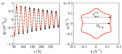
Figure 4: (a) Numerically obtained LDOS oscillations (points) at energy $E=330$ meV for the case when the line defect is perpendicular to the $\Gamma K$ direction, and the fit of $f(x)=A\sin(kx+\varphi)/x^{1/2}$ with fitting parameters $A$, $k$ and $\varphi$ (solid red line). (b) Constant energy contour and the relevant wave numbers $k_{\rm nest}$ and $2k_{\Gamma K}$. The wave number of the oscillation in (a) is given by $k_{\rm nest}^{\Gamma K}$, as the oscillations with $2k_{\Gamma K}$ are fast decaying ($\propto x^{-3/2}$) due to the absence of backscattering.

Even though the line defect in the considered experiment Ref. BiTexp, was perpendicular to the $\Gamma M$ direction of the surface Brillouin zoneLDOS_Biswas , it is instructive, and regarding future experiments, potentially useful to consider the other high-symmetry case when the line defect is oriented perpendicular to the $\Gamma K$ direction. In Fig. 4, we demonstrate that both the wave vector and the decay characteristics of the LDOS standing waves we obtain from our numerical technique are in complete correspondence with the analytical results of asymptotic analysisJingWang ; Biswas_arxiv . Namely, the wave number of the oscillation is given by the extremal (maximal) perpendicular-to-defect width $k_{\rm nest}^{\Gamma K}$ of the constant energy contour, whereas the decay goes as $\delta\rho(x)\propto 1/\sqrt{x}$. Oscillations with $2k_{\Gamma K}$ are not seen in Fig. 4a presumably because they are fast decaying ($\propto x^{-3/2}$) due to the absence of backscatteringLDOS_Biswas .

In conclusion, we theoretically described pre-asymptotic electronic LDOS oscillations in the vicinity of a line defect on the surface of Bi₂Te₃, with wave number and decay characteristics markedly different from the asymptotic ones. The calculated energy dependence of the characteristic wave number of the LDOS oscillations is in line with STM data. In a general context, our study highlights the importance of pre-asymptotic calculation of the surface-state LDOS oscillations in the analysis and interpretation of STM experiments.

Note: While completing this manuscript, we became aware of a related work related on electronic standing waves on 3DTI surfaces. Our results partially overlap with those in Ref. related, . Apart from various details of the model, the major distinctive features of our work are (i) the interpretation of the results in terms of the properties of the group velocity (Fig. 3d-g), and (ii) the quantitative agreement with the experimental results reported in Ref. BiTexp, .

Appendix A Band-structure parameters of the homogeneous system

To base our calculation on an accurate surface-state dispersion relation, in Sec. II. we estimated the band-structure parameters of Bi₂Te₃ by comparing the theoretical dispersion (see Eq. (2)) and DOS with the experimentally observed ARPES and STM spectra and the DOS derived from those. The four band-structure parameters are $v_{0}$, $\lambda$, $\gamma$ and $\alpha$. Here we outline the considerations we used for those estimates.

The signs of $\gamma$ and $\alpha$ can be determined by considering the ARPES spectrum along the $\Gamma M$ direction, shown as red crosses in Fig. 1a and b. Note that this cut of the dispersion relation corresponds to the function $\varepsilon_{+}(k_{x},0)$ in Eq. (2). The measured dispersion is linear for small wave number, its slope first becomes smaller as the wave number is increased, but then the slope increases again as wave number is increased further. This characteristic is naturally captured by a polynomial of the wave number with negative second-order coefficient and positive third-order coefficient. Since the third-order Taylor series of $\varepsilon_{+}(k_{x},0)$ in $k_{x}$ around zero has the form

$$\varepsilon_{+}(k_{x},0)\approx v_{0}k_{x}+\gamma k_{x}^{2}+\alpha v_{0}k_{x}^{3}$$ (16)

we can conclude that $\gamma<0$ and $\alpha>0$ is required to describe the measured dispersion. The signs of the remaining two parameters $v_{0}$ and $\lambda$ has no effect on the spectral properties, therefore we assign a positive sign to them.

Having the signs of band-structure parameters established, we determined the values of the four parameters by systematic visual comparison of the experimental dispersions (Figs. 1a,b), the DOS data obtained from ARPES and STM measurements (Figs. 1c,d of Ref. BiTexp, ), and the corresponding theoretical curves.

Appendix B Plane-wave states

We label the electronic plane-wave states by their energy $E$ and the parallel-to-defect wave-number component $q$, which are conserved in the scattering process on the line defect (for details see the main text). Here we review a numerical method to obtain these states, which is necessary to solve the scattering problem at the edge step. For a given $E$ and $q$ there are six solutions of longitudinal wave vector $k_{r,p}$ ($p=1\dots 6$) which satisfies the characteristic equation $\det\left[H(k_{r},q)-\rm{\hat{I}}E\right]=0$, where $\rm{\hat{I}}$ is the $2\times 2$ identity matrix and $H$ is the Hamiltonian defined by Eq. (1) in the main text. Complex roots $k_{r,p}$ of the characteristic polynomial

$$\det\left[H-\rm{\hat{I}}E\right]=\sum\limits_{k=0}^{6}a(E,q)k_{r}^{k}\;$$ (17)

are equal to eigenvalues of the companion matrix companion of this polynomial, hence we find the roots $k_{r,p}$ by numerically diagonalizing the companion matrix. Then, the spinor component $\chi$ of the corresponding plane wave $\Phi_{k_{r,p},q}(x,y)=e^{iqy}e^{ik_{r,p}x}\chi(k_{r,p},q)$ can be numerically computed from the eigenvalues problem

$$H(k_{r,p})\chi(k_{r,p},q)=E\chi(k_{r,p},q)$$ (18)

for $p=1,\dots,6$.

Appendix C Fourier analysis of $\delta\rho(x)$

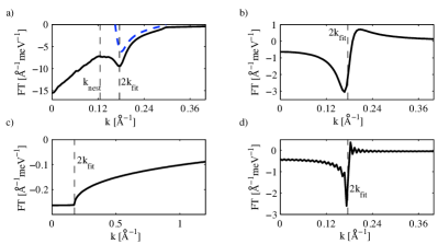
Figure 5: Comparison of the discrete Fourier transforms of (a) the computed LDOS oscillation $\delta\rho(x)$ shown in Fig. 3a, (b) the function $f_{2}(x)=A_{2}\sin(2k_{\rm fit}x+\varphi_{2})e^{-x/L}$, where $A_{2}$, $k_{\rm fit}$, $\varphi_{2}$, $L$ are obtained from fitting $f_{2}$ to $\delta\rho$, (c) $A_{2}\sin(2k_{\rm fit}x+\varphi_{2})x^{-3/2}$, and (d) $A_{2}\sin(2k_{\rm fit}x+\varphi_{2})x^{-1/2}$.

In Sec. IV, we present numerical results for the defect-induced spatial modulation of the LDOS, $\delta\rho(x)$. In order to develop an understanding of the decay characteristic of the LDOS oscillations, we fit a power-law decaying ($\delta\rho\propto x^{-3/2}$) as well as an exponentially decaying function, $f_{1}$ and $f_{2}$, respectively, to our data. According to Fig. 3a, the exponentially decaying $f_{2}$ provides a better fit, hinting that the decay characteristics is closer to an exponential than to a power-law predicted earlierLDOS_Zhou ; LDOS_Biswas ; Biswas_arxiv ; JingWang . However, our fitting procedure is not conclusive, as the exponentially decaying function $f_{2}$ has an extra fitting parameter, the length scale $L$ of the decay.

In order to investigate the decay characteristics further, here we provide the discrete Fourier transform (FT) (Fig. 5a) of the real-space data in Fig. 3a, and compare that to discrete Fourier transformed oscillations that decay in an exponential (Fig. 5b) or power-law (Fig 5c,d) fashion. The discrete Fourier transformation is carried out after symmetrization of the real-space data, i.e., after mapping the real-space data set $f(x_{i})$ $(i=0,\dots,N-1)$ to $f_{{\rm sym},j}$ ($j=0,\dots,2N-1$) via the definition

$$f_{{\rm sym},j}:=\left\{\begin{array}[]{cl}f(x_{j})&\mbox{if $0\leq j\leq N-1$,}\\ f(x_{2N-1-j})&\mbox{if $N\leq j\leq 2N-1$}.\end{array}\right.$$ (19)

This symmetrization ensures that the Fourier transform will be real valued in the large $N$ limit.

The subplots of Fig. 5 show the FT of (a) our numerical results $\delta\rho(x)$ shown in Fig. 3a, (b) the function $f_{2}(x)=A_{2}\sin(2k_{\rm fit}x+\varphi_{2})e^{-x/L}$, where $A_{2}$, $k_{\rm fit}$, $\varphi_{2}$, $L$ are obtained from fitting $f_{2}$ to $\delta\rho$, (c) $A_{2}\sin(2k_{\rm fit}x+\varphi_{2})x^{-3/2}$, and (d) $A_{2}\sin(2k_{\rm fit}x+\varphi_{2})x^{-1/2}$. The data in Fig. 5c,d shows, in accordance with the known analytical formula describing the Fourier transform of power-law decaying sinusoidal oscillationsLDOS_Biswas , that the FT develops non-analytical behavior at the characteristic wave number $2k_{\rm fit}$. In contrast, our data set in Fig. 5a shows no such non-analytical behavior, similarly to the FT of the exponentially decaying oscillation in Fig. 5b. This observation, although still not conclusive, further supports the possibility that the LDOS oscillations in the vicinity of the line defect do not follow a power-law decay, and perhaps are closer to an exponential. Further analytical studies, e.g., the extension of the asymptotic analysis LDOS_Biswas ; Biswas_arxiv ; JingWang to the pre-asymptotic spatial region might help settling this open issue.

In Sec. IV, we argued that the pre-asymptotic component of the LDOS is due to the interference of incoming and reflected partial waves i.e., that the role of evanescent and transmitted partial waves is negligible. To strengthen that point further, we plot the quantity

$$\tilde{\rho}_{r}(2k)=\frac{{\rm Re}\left(r_{k,q^{\prime}}\chi^{\dagger}_{k,q^{\prime}}\chi_{-k,q^{\prime}}\right)}{2\pi\hbar|v_{\parallel}(E,k)|}$$ (20)

as a function of $k$ [for definitions, see around Eq. (13)], as a dashed blue line in Fig. 5a. Note that $\tilde{\rho}_{r}(2k)$ is the Fourier transform of the symmetrized $\rho_{r}(x)$ of Eq. (13). Figure 5a further supports the interpretation that the dip around the characteristic wave number $2k_{\rm fit}$ of the LDOS oscillation forms as a result of interference of incoming and reflected partial waves.

References

- (1) M. Z. Hasan and C. L. Kane, Rev. Mod. Phys. 82, 3045 (2010).
- (2) D. Hsieh, D. Qian, L. Wray, Y. Xia, Y. S. Hor, R. J. Cava and M. Z. Hasan, Nature 452, 970 (2008).
- (3) D. Hsieh et al., Science 323, 919 (2009).
- (4) Y. Xia et al., Nat. Phys. 5, 398 (2009).
- (5) Y. L. Chen et al., Science 325, 178 (2009).
- (6) D. Hsieh et al., Phys. Rev. Lett. 103, 146401 (2009).
- (7) K. Kuroda, M. Arita, K. Miyamoto, M. Ye, J. Jiang, A. Kimura, E. E. Krasovskii, E. V. Chulkov, H. Iwasawa, T. Okuda, K. Shimada, Y. Ueda, H. Namatame and M. Taniguchi Phys. Rev. Lett. 105, 076802 (2010).
- (8) P. Roushan, J. Seo, C. V. Parker, Y. S. Hor, D. Hsieh, D. Qian, A. Richardella, M. Z. Hasan, R. J. Cava and A. Yazdani, Nature 460, 1106 (2009).
- (9) T. Zhang et al., Phys. Rev. Lett. 103, 266803 (2009).
- (10) J. Seo, P. Roushan, H. Beidenkopf, Y. S. Hor, R. J. Cava and A. Yazdani, Nature 466, 343 (2010).
- (11) Z. Alpichshev, J. G. Analytis, J.-H. Chu, I. R. Fisher, Y. L. Chen, Z. X. Shen, A. Fang and A. Kapitulnik, Phys. Rev. Lett. 104, 016401 (2010).
- (12) J. Wang, W. Li, P. Cheng, C. Song, T. Zhang, P. Deng, X. Chen, X. Ma, K. He, J.-F. Jia, Q.-K. Xue, B.-F. Zhu, Phys. Rev. B 84, 235447 (2011).
- (13) M. F. Crommie, C. P. Lutz and D. M. Eigler, Nature 363, 524 (1993).
- (14) L. Fu, Phys. Rev. Lett. 103, 266801 (2009).
- (15) W.-C. Lee, C. Wu, D. P. Arovas and S.-C. Zhang, Phys. Rev. B 80, 245439 (2009).
- (16) H. M. Guo and M. Franz, Phys. Rev. B 81, 041102(R) (2010).
- (17) Q.-H. Wang, D. Wang and F.-C. Zhang, Phys. Rev. B 81, 035104 (2010).
- (18) X. Zhou, C. Fang, W. F. Tsai, and J. P. Hu, Phys. Rev. B 80, 245317 (2009).
- (19) R. R. Biswas and A. V. Balatsky, Phys. Rev. B 83, 075439 (2011).
- (20) R. R. Biswas and A. V. Balatsky, arXiv:1005.4780 (unpublished).
- (21) Q. Liu, arXiv:1108.6051 (unpublished).
- (22) S. Basak, H. Lin, L. A. Wray, S.-Y. Xu, L. Fu, M. Z. Hasan, and A. Bansil, Phys. Rev. B 84, 121401(R) (2011).
- (23) S. Datta, Electronic Transport in Mesoscopic Systems (Cambridge University Press, 1995).
- (24) D. Zhang and C. S. Ting, Phys. Rev. B 85, 115434 (2012).
- (25) R. A. Horn and C. R. Johnson, Matrix Analysis (Cambridge University Press, 1985).