Achlioptas processes are not always self-averaging

Abstract

We consider a class of percolation models, called Achlioptas processes, discussed in [Science 323, 1453 (2009)] and [Science 333, 322 (2011)]. For these the evolution of the order parameter (the rescaled size of the largest connected component) has been the main focus of research in recent years. We show that, in striking contrast to ‘classical’ models, self-averaging is not a universal feature of these new percolation models: there are natural Achlioptas processes whose order parameter has random fluctuations that do not disappear in the thermodynamic limit.

I Introduction

Percolation is a fundamental problem in statistical physics, and the emergence of long range connectivity in various percolation models is one of the quintessential examples of a phase transition. While many ‘classical’ models and their broad universality classes are nowadays well understood Stauffer and Aharony (1994); Grimmett (1999); Bollobás and Riordan (2006), in recent years a new class of percolation models has been widely studied. These so-called Achlioptas processes Achlioptas et al. (2009); Bohman and Kravitz (2006); Spencer and Wormald (2007); Riordan and Warnke (2011a) are defined via a slight modification of well-studied Erdős–Rényi random graphs, and have been of great interest to many physicists Achlioptas et al. (2009); Ziff (2009); Cho et al. (2009); Radicchi and Fortunato (2009); Friedman and Landsberg (2009); Radicchi and Fortunato (2010); D’Souza and Mitzenmacher (2010); Cho et al. (2010); Ziff (2010); da Costa et al. (2010); Manna and Chatterjee (2011); Nagler et al. (2011); Araújo et al. (2011); Chen and D’Souza (2011); Hooyberghs and Van Schaeybroeck (2011); Andrade et al. (2011); Grassberger et al. (2011); Riordan and Warnke (2011b); Lee et al. (2011); Choi et al. (2011); Bastas et al. (2011); Cho and Kahng (2011); Tian and Shi (2012); Manna (2012) due to their intriguingly different features.

One of the most studied properties of Achlioptas processes is the evolution of the order parameter (the rescaled size of the largest connected component), yielding several surprises Achlioptas et al. (2009); da Costa et al. (2010); Riordan and Warnke (2011a, b). Indeed, certain Achlioptas processes were first claimed to have discontinuous (first order) phase transitions Achlioptas et al. (2009), in striking contrast to the typical second order transition observed in classical percolation models. Called explosive percolation, this was subsequently supported by many researchers Ziff (2009); Cho et al. (2009); Radicchi and Fortunato (2009); Friedman and Landsberg (2009); D’Souza and Mitzenmacher (2010); Radicchi and Fortunato (2010); Cho et al. (2010); Ziff (2010); Hooyberghs and Van Schaeybroeck (2011), but recently it was mathematically rigorously proven that the transition is in fact continuous for all mean-field Achlioptas processes Riordan and Warnke (2011a, b), although it can be extremely steep da Costa et al. (2010). Furthermore, compared to the classical cases many of these models seem to behave differently in essential ways, representing a new universality class da Costa et al. (2010); Grassberger et al. (2011); Bastas et al. (2011); Tian and Shi (2012) whose basic features still require further investigation Bohman (2009); Janson (2011).

In this letter we show that these new percolation models can show another surprising behaviour: there are natural Achlioptas processes whose order parameter has large random fluctuations, i.e., is not self-averaging. This is in contrast to classical models, where the order parameter converges to a nonrandom function in the thermodynamic limit. As our nonconvergent examples are from different universality classes, including the ‘explosive’ one, these also serve as a cautionary tale: when studying a wide range of Achlioptas processes, one should not take convergence for granted.

II The Model

Many ‘competitive’ percolation models on the complete graph have been studied, see e.g. Achlioptas et al. (2009); Bohman and Kravitz (2006); Spencer and Wormald (2007); da Costa et al. (2010); D’Souza and Mitzenmacher (2010); Nagler et al. (2011); Riordan and Warnke (2011a) and the references therein. These Achlioptas processes start, as in the classical Erdős–Rényi (ER) model, with an empty graph consisting of a large number $n$ of isolated vertices, and then sequentially add random edges to the graph. In the simplest case in every round two random edges $e_{1}=v_{1}v_{2}$ and $e_{2}=v_{3}v_{4}$ are picked (rather than one), and, using some rule, one of them is chosen and added to the evolving graph. Of course, there is nothing special about two edges; indeed, Achlioptas processes are a subset of the general class of $\ell$-vertex rules introduced in Riordan and Warnke (2011a). Here in every round $\ell$ uniformly random vertices $v_{1},\ldots,v_{\ell}$ are chosen, and two of them are connected with an edge using some rule (see Riordan and Warnke (2011a) for more variations). Note that the resulting percolation processes include the ER model, which we obtain by always adding $v_{1}v_{2}$.

In the following we introduce two different $3$-vertex rules belonging to different universality classes, always writing $c_{i}$ for the size of the component containing $v_{i}$. The first rule, the NG rule, proceeds as follows. If all three component sizes $c_{i}$ are equal, add $v_{1}v_{2}$. If exactly two component sizes $c_{i}$ are equal, connect the corresponding vertices with an edge. Otherwise (if all $c_{i}$ are different) join the vertices in the two smallest components. This rule is named after Nagler and Gutch, who suggested a slight variant in a different context (personal communication). It is a modification of the ‘explosive’ triangle rule introduced in Friedman and Landsberg (2009); D’Souza and Mitzenmacher (2010), which has a steep (but continuous) transition. The rapid growth of the order parameter in Figure 3 shows that NG also belongs to the class of ‘explosive’ rules.

The second rule we consider can be viewed as a modified ER model and thus we use the shorthand mER. Writing $L_{1}$ and $L_{2}$ for the sizes of the two largest components of the evolving graph, it is defined as follows. If the two largest components in the current graph have the same size ($L_{1}=L_{2}$), add $v_{1}v_{2}$. When $L_{1}>L_{2}$, if at least two $c_{i}$ are equal to $L_{1}$, connect two corresponding vertices; otherwise connect two vertices in components of size smaller than $L_{1}$. Figure 3 indicates that mER belongs to the class of ‘nonexplosive’ rules, where the order parameter evolves rather slowly around the percolation threshold (as in the classical ER case).

III Results

For Achlioptas processes the natural order parameter is

$$\rho_{n}(t)=\frac{L_{1}(tn)}{n},$$

where $L_{1}(m)$ denotes the size of the largest connected component after $m$ steps (suppressing in the notation the dependence on the rule ${\mathcal{R}}$ and on the number of vertices $n$). For classical percolation models it is well known that the order parameter converges to a nonrandom function in the thermodynamic limit, i.e., that there exists a scaling limit $\rho:[0,\infty)\to[0,1]$ such that

$$\lim_{n\to\infty}\rho_{n}(t)=\rho(t).$$ (1)

Since $L_{1}(tn)$ is random, this actually means that $\rho_{n}(t)=L_{1}(tn)/n$ converges in probability to $\rho(t)$, see e.g. Riordan and Warnke (2011a) for a more detailed discussion. So (1) asserts: (A) that $\rho_{n}(t)$ is self-averaging, i.e., that the random fluctuations are negligible as $n\to\infty$, and (B) that the expected value of $\rho_{n}(t)$ converges to some deterministic function, i.e., that ${\mathbb{E}}\rho_{n}(t)$ does not depend on $n$ in the thermodynamic limit.

In the following we show that for the NG and mER rules the corresponding scaling limits do not exist, i.e., that (1) fails. To establish this we estimate the mean $\mu_{n}$ and standard deviation $\sigma_{n}$ of $\rho_{n}(1)$ for a range of $n$ (based on $10^{4}$ runs for each $n$). Formally we say that $\rho_{n}(t)$ is self-averaging (at time $t=1$) if $\sigma_{n}/\mu_{n}\to 0$ as $n\to\infty$, which is well known to hold for the ER process (see also Figure 1). For the NG rule, and especially the mER rule, Figure 1 demonstrates that $\sigma_{n}/\mu_{n}$ does not tend to $0$ in the thermodynamic limit; hence these are not self-averaging. This is further illustrated in Figure 2, which also indicates that the expected values of the corresponding order parameters have a non-trivial dependence on $n$: they seem to oscillate. While for the mER rule the amplitudes seem to vanish in the thermodynamic limit, for the NG rule we leave it open whether ${\mathbb{E}}\rho^{\mathrm{NG}}_{n}(t)$ converges as $n\to\infty$ or not: if it does, then Figure 2 suggests that this only happens for extremely large values of $n$.

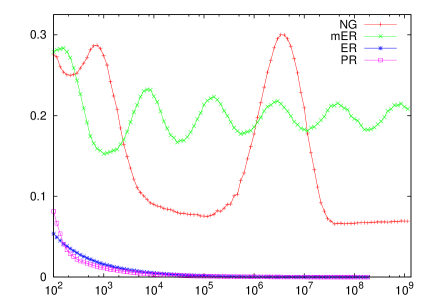
Figure 1: (Color online). Estimated value of $\sigma_{n}/\mu_{n}$ for $\rho_{n}(1)$ as a function of $n$ (each based on $10^{4}$ runs) using the NG, mER, ER rules and product rule (PR) Achlioptas et al. (2009). Self-averaging (ER, PR) does not correlate with being ‘explosive’ (NG, PR).

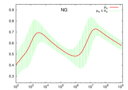
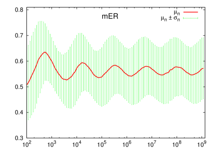
Figure 2: (Color online). Simulation of the order parameter $\rho_{n}(1)=L_{1}(n)/n$ as a function of $n$ for the NG and mER rules: average and standard deviation ($10^{4}$ runs for each $n$).

To put our findings into perspective, note that it is easy to construct artificial Achlioptas processes without scaling limits (using, for example, different rules depending on the vertices sampled in the first round). The point is that the mER, and in particular the NG rule, are natural examples which nevertheless are nonconvergent. Furthermore, they belong to two very different classes of rules (explosive and nonexplosive). This shows that, contrary to classical percolation models, self-averaging is not a universal feature of Achlioptas processes.

IV Analysis

We start by collecting some structural properties of Achlioptas processes. Remark 9 in Riordan and Warnke (2011a) implies that whp (meaning with high probability, i.e., with probability tending to $1$ as $n\to\infty$) the following two properties hold throughout the entire evolution of any $\ell$-vertex Achlioptas process: (i) the vertex set of the union of the $\ell-1$ largest components changes by at most $o(n)$ vertices in any $o(n)$ steps, and (ii) there exists a function $s=s(n)$ such that the $\ell$-th largest component always has size at most $s=o(n)$. Although (i) might seem rather technical at first sight, it has an important implication: it shows that (whp) the size of the largest component can ‘jump’, i.e., change by $\Theta(n)$ vertices in $o(n)$ steps, only if there is a step where two linear size components merge to form the new largest component (for $\ell$-vertex rules this strengthens some of the main conclusions in Nagler et al. (2011)).

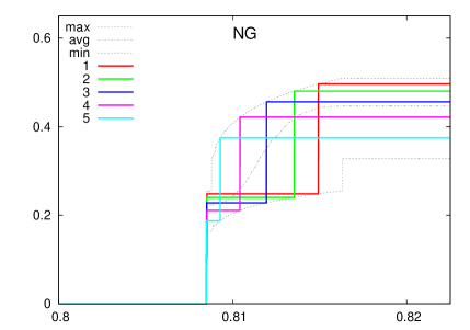
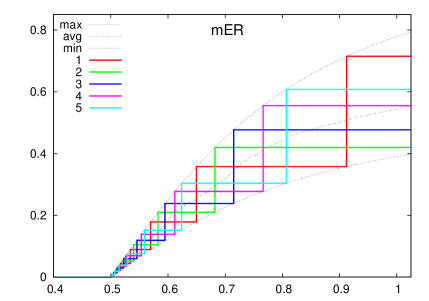
Figure 3: (Color online). Simulation of the order parameter $\rho_{n}(t)=L_{1}(tn)/n$ as a function of $t$ for the NG and mER rules with $n=10^{11}$: five sample runs together with min, max and average of $10^{3}$ runs.

Turning to the evolution of the NG and mER rules, the key property of both is that they prevent the largest component from growing as long as the two largest components have different sizes ($L_{1}>L_{2}$). But, whenever we have two linear size ‘giant’ components of the same size, they merge with constant probability in each step (recall that by property (ii) we can have at most two such components as here $\ell=3$). If this happens then $L_{1}$ doubles and by (ii) we are left with one giant; all other components, in particular $L_{2}$, have size at most $s=o(n)$. Now $L_{1}$ is prevented from growing and $L_{2}$ slowly starts growing. After some time $L_{2}$ emerges to linear size, while all smaller components have size at most $s=o(n)$ by (ii). When $L_{1}$ and $L_{2}$ have similar size, they might overtake each other repeatedly, but since we have many small components they will merge in $o(n)$ steps, and again $L_{1}$ essentially doubles by property (i). To summarize, after the first linear size giant appears, the remaining evolution of $L_{1}$ is essentially governed by discrete doublings.

The behaviour at the percolation threshold, where the first linear size component is formed, seems rather complicated for both rules. However, the simulation results for the NG and mER rules depicted in Figure 3 show that the size of the linear size giant component is not deterministic once it first emerges: note the large spread in the order parameter $\rho_{n}(t)=L_{1}(tn)/n$. So, after the percolation threshold the largest component has random size. Since the remaining discrete doublings depend on this initial value, this shows that the corresponding $\rho^{\mathrm{NG}}_{n}(t)$ and $\rho^{\mathrm{mER}}_{n}(t)$ exhibit large random fluctuations in their subsequent evolution. Figures 1 and 2 indicate that these do not disappear in the thermodynamic limit: the order parameters of the NG and mER rules are not self-averaging. This ‘freezing in’ of early variations (the microscopic fluctuations in the size of the largest component are magnified and propagated to later in the process) is similar to the nonconvergent behaviour of the maximum degree in the Barabási–Albert network model Barab si and Albert (1999), see e.g. Bollobás and Riordan (2003).

For the mER rule we can formally describe this propagation to later stages, since its evolution has a close connection to Erdős–Rényi random graphs. To see this, we first argue that throughout its evolution, up to $o(n)$ differences, mER yields a graph of the following form: its largest component has size $\alpha n$, where $\alpha\geq 0$, and the remaining smaller component sizes follow the distribution of an ER graph $G(\tilde{n},\lambda/\tilde{n})$ where $\tilde{n}=(1-\alpha)n$ and $\lambda\geq 0$; here $G(n,p)$ denotes the binomial random graph model in which, starting with an empty graph on $n$ vertices, each of the $\binom{n}{2}$ possible edges is included independently with probability $p$ (for $p=2m/n^{2}$ it is well known to be very similar to the uniform ER graph obtained after inserting $m$ random edges). The key observation is that whenever $L_{1}>L_{2}$, the mER rule either adds an edge with both ends inside the largest component, or one with both ends outside. In each case the endpoints are chosen uniformly at random. So, between each doubling of $L_{1}$ the graph outside the largest component evolves like a (rescaled) ER graph. Once $L_{1}$ and $L_{2}$ have similar linear size they merge in $o(n)$ steps, so, for equality up to $o(n)$ differences, it suffices to show that the step in which they merge retains the claimed form of the graph. But this follows from the discrete duality principle for $G(n,c/n)$ first used in Bollobás (1984): the removal of the largest component leaves an ER graph $G(n^{\prime},d/n^{\prime})$ on $n^{\prime}$ vertices with $d\leq 1$. Summarizing, the evolution of the mER graph after $m=tn$ steps is described by the evolution of the parameters $\alpha(t)$ and $\lambda(t)$, which control the size of the largest component and the distribution of the smaller component sizes, respectively. For $t\leq 1/2$ we have $\alpha=0$ and $\lambda=2t$: the graph is still close to the ER graph (as all components are small). Close to $t=1/2$ the parameters evolve in a non-deterministic way. Then, as a function of this ‘initial randomness’ at time $t_{0}>1/2$, the later evolution is deterministic and can be described explicitly for any $t\geq t_{0}$. For the mER rule this explains how the lack of self-averaging depicted in Figure 3 arises.

Finally, the ‘jumps’ of the order parameter in Figure 3 show that the NG and mER rules are examples of Achlioptas processes which violate ($\star$) continuity throughout the process, although these satisfy the widely studied ($\dagger$) continuity at the percolation threshold by Riordan and Warnke (2011a, b). In fact, since in both rules the largest component grows essentially only by discrete doublings, it follows that after the percolation threshold both give rise to an ‘infinite’ number of discontinuities in sense ($\star$). Property (i) implies that in $\ell$-vertex rules such discontinuities can only arise if two linear size components merge. It would be interesting to know if, when restricting to $\ell$-vertex rules whose decisions (which edge to add) depend only on the component sizes $(c_{1},\ldots,c_{\ell})$, this is the only mechanism leading to nonconvergent behaviour.

V Conclusions

In summary, we have shown that self-averaging of the order parameter is not a universal feature of Achlioptas processes: the corresponding scaling limits do not always exist. While for any particular rule this can be tested numerically via simulations (as in Grassberger et al. (2011); Lee et al. (2011) for example), the large interest in such percolation models Achlioptas et al. (2009); Ziff (2009); Cho et al. (2009); Radicchi and Fortunato (2009); Friedman and Landsberg (2009); Radicchi and Fortunato (2010); D’Souza and Mitzenmacher (2010); Cho et al. (2010); Ziff (2010); da Costa et al. (2010); Manna and Chatterjee (2011); Nagler et al. (2011); Araújo et al. (2011); Chen and D’Souza (2011); Hooyberghs and Van Schaeybroeck (2011); Andrade et al. (2011); Grassberger et al. (2011); Riordan and Warnke (2011b); Lee et al. (2011); Choi et al. (2011); Bastas et al. (2011); Cho and Kahng (2011); Tian and Shi (2012); Manna (2012) indicates that a theoretical investigation of convergence in Achlioptas processes is needed, see also Bohman (2009); Janson (2011). Is there a general criterion which allows us to determine whether certain rules are convergent or not? Recently self-averaging has been rigorously established for a restricted class of Achlioptas rules Riordan and Warnke (2011c): this includes the ‘dCDGM’ rule considered in da Costa et al. (2010), but not the widely studied Achlioptas et al. (2009); Ziff (2009); Cho et al. (2009); Radicchi and Fortunato (2009); Friedman and Landsberg (2009); Radicchi and Fortunato (2010); Cho et al. (2010); Ziff (2010); Manna and Chatterjee (2011); Nagler et al. (2011); Araújo et al. (2011); Hooyberghs and Van Schaeybroeck (2011); Andrade et al. (2011); Grassberger et al. (2011); Riordan and Warnke (2011b); Lee et al. (2011); Choi et al. (2011); Bastas et al. (2011); Cho and Kahng (2011); Tian and Shi (2012); Manna (2012) product rule (PR). Simulations indicate that the scaling limit of the PR rule most likely exists (see e.g. Figure 1), but given the surprises that it has shown so far Achlioptas et al. (2009); Bohman (2009); Riordan and Warnke (2011b); Janson (2011) we can only be sure once we have rigorous results.

References

- Stauffer and Aharony (1994) D. Stauffer and A. Aharony, Introduction To Percolation Theory, 2nd ed. (Taylor & Francis Ltd., London, 1994).
- Grimmett (1999) G. Grimmett, Percolation, 2nd ed. (Springer-Verlag, Berlin, 1999).
- Bollobás and Riordan (2006) B. Bollobás and O. Riordan, Percolation (Cambridge University Press, New York, 2006).
- Achlioptas et al. (2009) D. Achlioptas, R. M. D’Souza, and J. Spencer, Science 323, 1453 (2009).
- Bohman and Kravitz (2006) T. Bohman and D. Kravitz, Combin. Probab. Comput. 15, 489 (2006).
- Spencer and Wormald (2007) J. Spencer and N. Wormald, Combinatorica 27, 587 (2007).
- Riordan and Warnke (2011a) O. Riordan and L. Warnke, Ann. Appl. Probab., to appear (2011a), arXiv:1102.5306 .
- Ziff (2009) R. M. Ziff, Phys. Rev. Lett. 103, 045701 (2009).
- Cho et al. (2009) Y. S. Cho, J. S. Kim, J. Park, B. Kahng, and D. Kim, Phys. Rev. Lett. 103, 135702 (2009).
- Radicchi and Fortunato (2009) F. Radicchi and S. Fortunato, Phys. Rev. Lett. 103, 168701 (2009).
- Friedman and Landsberg (2009) E. J. Friedman and A. S. Landsberg, Phys. Rev. Lett. 103, 255701 (2009).
- Radicchi and Fortunato (2010) F. Radicchi and S. Fortunato, Phys. Rev. E 81, 036110 (2010).
- D’Souza and Mitzenmacher (2010) R. M. D’Souza and M. Mitzenmacher, Phys. Rev. Lett. 104, 195702 (2010).
- Cho et al. (2010) Y. S. Cho, S.-W. Kim, J. D. Noh, B. Kahng, and D. Kim, Phys. Rev. E 82, 042102 (2010).
- Ziff (2010) R. M. Ziff, Phys. Rev. E 82, 051105 (2010).
- da Costa et al. (2010) R. A. da Costa, S. N. Dorogovtsev, A. V. Goltsev, and J. F. F. Mendes, Phys. Rev. Lett. 105, 255701 (2010).
- Manna and Chatterjee (2011) S. Manna and A. Chatterjee, Physica A 390, 177 (2011).
- Nagler et al. (2011) J. Nagler, A. Levina, and M. Timme, Nature Phys. 7, 265 (2011).
- Araújo et al. (2011) N. A. M. Araújo, J. S. Andrade, R. M. Ziff, and H. J. Herrmann, Phys. Rev. Lett. 106, 095703 (2011).
- Chen and D’Souza (2011) W. Chen and R. M. D’Souza, Phys. Rev. Lett. 106, 115701 (2011).
- Hooyberghs and Van Schaeybroeck (2011) H. Hooyberghs and B. Van Schaeybroeck, Phys. Rev. E 83, 032101 (2011).
- Andrade et al. (2011) J. S. Andrade, H. J. Herrmann, A. A. Moreira, and C. L. N. Oliveira, Phys. Rev. E 83, 031133 (2011).
- Grassberger et al. (2011) P. Grassberger, C. Christensen, G. Bizhani, S.-W. Son, and M. Paczuski, Phys. Rev. Lett. 106, 225701 (2011).
- Riordan and Warnke (2011b) O. Riordan and L. Warnke, Science 333, 322 (2011b).
- Lee et al. (2011) H. K. Lee, B. J. Kim, and H. Park, Phys. Rev. E 84, 020101 (2011).
- Choi et al. (2011) W. Choi, S.-H. Yook, and Y. Kim, Phys. Rev. E 84, 020102 (2011).
- Bastas et al. (2011) N. Bastas, K. Kosmidis, and P. Argyrakis, Phys. Rev. E 84, 066112 (2011).
- Cho and Kahng (2011) Y. S. Cho and B. Kahng, Phys. Rev. Lett. 107, 275703 (2011).
- Tian and Shi (2012) L. Tian and D.-N. Shi, Phys. Lett. A 376, 286 (2012).
- Manna (2012) S. S. Manna, Physica A 391, 2833 (2012).
- Bohman (2009) T. Bohman, Science 323, 1438 (2009).
- Janson (2011) S. Janson, Science 333, 298 (2011).
- Barab si and Albert (1999) A.-L. Barab si and R. Albert, Science 286, 509 (1999).
- Bollobás and Riordan (2003) B. Bollobás and O. Riordan, in Handbook of graphs and networks (Wiley-VCH, Weinheim, 2003) pp. 1–34.
- Bollobás (1984) B. Bollobás, Trans. Amer. Math. Soc. 286, 257 (1984).
- Riordan and Warnke (2011c) O. Riordan and L. Warnke, Preprint (2011c), arXiv:1111.6179 .