Barrow and Leibniz on the fundamental theorem of the Calculus

Abstract.

In 1693, Gottfried Whilhelm Leibniz published in the Acta Eruditorum a geometrical proof of the fundamental theorem of the calculus. During his notorious dispute with Isaac Newton on the development of the calculus, Leibniz denied any indebtedness to the work of Isaac Barrow. But it is shown here, that his geometrical proof of this theorem closely resembles Barrow’s proof in Proposition 11, Lecture 10, of his Lectiones Geometricae, published in 1670.

1. Introduction

At the height of his priority dispute with Newton concerning the invention of the calculus, Leibniz wrote an account, Historia et Origo Calculi Differentialis, describing the contributions by seventeenth century mathematicians that led him to his own development of the calculus (Child 1920, 22). In this account, Isaac Barrow is not mentioned at all, and in several occasions Leibniz denied any indebtedness to his work, particularly during his notorious priority dispute with Isaac Newton. But in Barrow’s Lectiones Geometricae (hereafter cited as Geometrical Lectures), which Leibniz had obtained during a visit to London in 1673, the concepts of the differential and integral calculus are discussed in geometrical form, and a rigorous mathematical proof is given of the fundamental theorem of the calculus . According to J. M. Child, “a Calculus may be of two kinds:

i) An analytic calculus, properly so called, that is, a set of algebraical working rules (with their proofs), with which differentiations of known functions of a dependent variable, of products, of quotients, etc., can be carried out; together with the full recognition that differentiation and integration are inverse operations, to enable integration from first principles to be avoided . . .

ii) A geometrical calculus equivalent embodying the same principles and methods; this would be the more perfect if the construction for tangents and areas could be immediately translated into algebraic form, if it where so desired.

Child concludes

Between these two there is, in my opinion, not a pin to choose theoretically; it is a mere matter of practical utility that set the first type in front of the second; whereas the balance of rigour, without modern considerations, is all on the side of the second ( Child 1930, 296).

More recently, a distinguished mathematician, Otto Toeplitz, wrote that “ Barrow was in possesion of most of the rules of differentiation, that he could treat many inverse tangent problem (indefinite integrals), and that in 1667 he discovered and gave an admirable proof of the fundamental theorem - that is the relation [ of the inverse tangent] to the definite integral (Toeplitz 1963, 128).

Leibniz’s original work concerned the analytic calculus, and he claimed to have read the relevant sections of Barrow’s lectures on the geometrical calculus only several years later, after he had independently made his own discoveries. In a letter to Johann Bernoulli written in 1703 , he attributed his initial inspiration to a “characteristic triangle” he had found in Pascal’s Traité des sinus du quart the cercle. After examining Leibniz’s original manuscript, and his copy of Barrow’s Geometrical Lectures, which were not available to Child, D. Mahnke (Manhke 1926) concluded that Leibniz had read only the beginning of this book, and that his calculus discoveries were made independently of Barrow’s work. Later, J. E. Hofmann (Hofmann 1974), likewise concluded that this independence is confirmed from Leibniz’s early manuscripts and correspondence at the time (Hofmann 1974).

In his early mathematical studies, Leibniz considered number sequences and realized that the operations associated with certain sums and differences of these sequences had a reciprocal relation. Then, by approximating a curve by polygons, these sums correspond to the area bounded by the curve, while the differences correspond to its tangent, (Bos 1973; Bos 1986, 103), which Leibniz indicated , lead to his insight of the reciprocal relation between areas and tangents . For example, Leibniz’s June 11, 1677 letter addressed to Oldenburg for Newton, in reply to Newton’s October 24, 1676 letter to Leibniz (Epistola Posterior), clearly shows that by this time he understood the fundamental theorem of the calculus, and its usefulness to evaluate algebraic integrals (Newton 1960, 221; Guicciardini 209, 360). But Child has given considerable circumstantial evidence, based on the reproductions of some of Leibniz’s manuscripts, that Barrow’s Geometrical Lectures also influenced some of Leibniz’s work (Child 1920), and he did not concur with Mahnke’s conclusion. To give one example, in the first publication of his integral calculus (Leibniz 1686), Leibniz gave an analytic derivation of Barrow’s geometrical proof in Prop. 1, Lecture 11, (Child 1916, 125), that the area bounded by a curve with ordinates equal to the subnormals of a given curve is equal to half of the square of the final ordinate of the original curve. In this publication, Leibniz admitted that he was familiar with Barrow’s theorem, and notes found in the margin of his copy of Barrow’s Lecciones Geometricae indicate that Leibniz had read it sometimes between 1674 and 1676 (Leibniz 2008, 301). Barrow’s proposition appears in one of he last lectures in his book, which suggests that by this time he had read also most of the other theorems in this book, particularly Prop. 11, Lecture 10 which contains Barrow’s geometrical proof of the fundamental theorem of the calculus.

But in a 1694 letter to the Marquis de l’Hospital, Leibniz wrote:

I recognize that M. Barrow has advanced considerably, but I can assure you, Sir, that I have derived no assistance from him for my methods (pour mes methodes) (Child 1920, 220),

and insisted that

by the use of the “characteristic triangle” . . . I thus found as it were in the twinkling of an eyelid nearly all the theorems that I afterward found in the works of Barrow and Gregory (Child 1920, 221).

Later, in an intended postscript to a letter from Berlin to Jacob Bernoulli, dated April 1703, he wrote,

Perhaps you will think it small-minded of me that I should be irritated with you, your brother [Johann Bernoulli], or anyone else, it you should have perceived the opportunities for obligation to Barrow, which it was not necessary for me, his contemporary in these discoveries to have obtained from him. (Child 1920, 11)

Apparently this comment was motivated by an article in the Acta Eruditorum of January 1691, where Jacob Bernoulli had emphasized the similarities of the methods of Barrow with those of Leibniz, and argued that anyone who was familliar with the former could hardly avoid recognizing the latter,

Yet to speak frankly, whoever has understood Barrrow’s . . . will hardly fail to know the other discoveries of Mr. Leibniz considering that they were based on that earlier discovery, and do not differ from them, except perhaps in the notation of the differentials and in some abridgment of the operation of it.(Feingold 1993, 325)

More recently, M. S. Mahoney, presumably referring to Child’s work, remarked that “Barrow seems to have acquired significant historical importance only at the turn of the twentieth century, when historians revived his reputation on two grounds: as a forerunner of the calculus and as a source of Newton’s mathematics.” But, he continued, “beginning in the 1960’s two lines of historical inquiry began to cast doubt on this consensus” , and he concluded that Barrow was “ competent and well informed, but not particularly original” (Mahoney 1990, 180, 240). This sentiment echoes Whiteside’s assessment that “Barrow remains . . . only a thoroughly competent university don whose real importance lies more in his coordinating of available knowledge for future use rather than in introducing new concepts” (Whiteside 1961, 289). In contrast to these derogatory comments, Toeplitz concluded, in conformance with Child’s evaluation, that “in a very large measure Barrow is indeed the real discoverer [of the fundamental theorem of the calculus] - insofar as an individual can ever be given credit within a course of development such as we have tried to trace here” (Toeplitz 1963, 98). Whiteside claimed that Barrow’s proof of the fundamental theorem of the calculus is only a “neat amendment of [James] Gregory’s generalization of Neil’s rectification method,” where Barrow “merely replaced an element of arc length by the ordinate of a curve.” But M. Feingold has pointed out that Whiteside’s claim that Barrow borrowed results from Gregory is not consistent with the fact that Barrow’s manuscript was virtually finished and already in the hands of John Collins, who shepherded it trough the publication process by the time that Barrow received Gregory’s book(Feingold 1993, 333).

This article is confined primarily to Leibniz geometrical discussion of the fundamental theorem of the calculus as it appeared in the 1693 Acta Eruditorum, and to a detailed comparison with Barrow’s two proofs of this theorem in Proposition 11, Lecture 10, and in Prop. 19, Lecture 11, published in his Geometrical Lectures 23 years earlier. In particular, Leibniz’s early development of the analytic form of the calculus, and his introduction of the suggestive notation that is in use up to the present time, will not be discussed here, and likewise, the related work of Isaac Newton, which recently has been covered in great detail by N. Guicciardini in his book Isaac Newton on Mathematical Certainty and Method, that contains also an excellent set of references to earlier work on this subject (Guicciardini 2009) In the next section, Barrow’s geometrical proofs of these two propositions is discussed, and in Section 3 the corresponding demonstration by Leibniz is given, showing its close similarity to Barrow’s work. This resemblance has not been discussed before, although it was noticed recently by L. Giacardi (Giacardi 1995), and it supports Child’s thesis that some of Leibniz’s contributions to the development of the calculus were influenced by Barrow’s work. Section 4 gives a description of an ingenious mechanical device invented by Leibniz to obtain the area bounded by a given curve, and Section 5 contains a brief summary and conclusions. In Appendix A a detailed discussion is given of Barrow’s proposition 1, Lecture 11, that illustrates his application of the characteristic triangle, which Leibniz obtained sometimes between 1674 and 1676. Finally, in Appendix B it is pointed out that significant errors occur in the reproduction of Leibniz’s diagram associated with the fundamental theorem as it appears in Gerhard’s edition (Leibniz 1693), in Struik’s English translation (Struik 1969, 282), and more recently in L. Giacardi’s book (Giacardi 1995), that apparently have remained unnoticed in the past.

2. Barrow’s geometrical proof of the fundamental theorem of the calculus

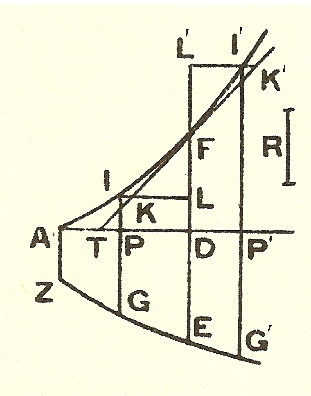
Figure 1. Barrow’s diagram for Proposition 11, Lecture 10. For clarity, prime superscripts have been added to labels that appear repeated in the original diagram.

In lectures 10 and 11 of his Geometrical Lectures, Barrow gave two related geometrical proofs of the fundamental theorem of the calculus, (Child 1916, 116,135; Struik 1969, 256; Mahoney 1990, 223,232; Folkerts 2001; Guicciardini 2009, 175). Underscoring the value of this theorem, he started his discussion with the remark

I add one or two theorems which it will be seen are of great generality, and not lightly to be passed over

Referring to his diagram in Prop. 11, Lecture 10, shown in Fig. 1, the area bounded by a given curve $ZGEG^{\prime}$ is described by another curve $AIFI^{\prime}$ with a common abscissa $APDP^{\prime}$. Barrow then proved that the subtangent $DT$ of $AIFI^{\prime}$ at $F$ is proportional to the ratio of the ordinates of the curves $AIFI^{\prime}$ and $ZGEG^{\prime}$, at a corresponding value $AD$ of the abscissa, i.e. $DT=R(DF/DE)$, where $R$ is an arbitrary parameter with dimensions of length. Even by modern standards, Barrow’s proof is mathematically rigorous, and it does not depend on any assumptions about differentials or infinitesimals which were not well understood at the time. In Proposition 19, Lecture 11, Barrow gave a related geometrical proof of his theorem that was based on an expression for the subtangent and for the area of curves in terms of differential quantities that were well known to mathematicians in the seventeenth century (Boyer, 1959).

Barrow started Prop. 11 with a description of his diagram, shown in Fig. 1, as follows:

Let $ZGE$ be any curve of which the axis is $AD$, and let ordinates applied to this axis $AZ,PG,DE$ continually increase from the initial coordinate $AZ$; and also let $AIF$ be a line [another curve] such that, if any line $EDF$ is drawn perpendicular to $AD$ cutting the curves in the points $E,F$, and $AD$ in $D$ the rectangle contained by $DF$ and a given length $R$ is equal to the intercepted space $ADEZ$;” (Child 1916, 117)

In other word, the ordinate $DF$ that determines the curve $AIFI^{\prime}$ is equal to the area $ADEZ$ bounded by the curve $ZGE$, the abcissa $AD$ and the ordinates $AZ$ and $DE$. Because the quantity associated with an area has the dimensions of length squared, Barrow introduced a parameter $R$ with units of length, and set

(1) $$DF=area(ADEZ)/R.$$

Barrow concluded,

also let $DE/DF=R/DT$, and join $DT$. Then $TF$ will touch the curve $AIF$(Child, 1916, 117),

which meant that $TF$ is a line tangent to the curve $AIF$ at $F$. Since it is $DE$ and $DF$ that are determined at a given valued of the abscissa $AD$, $DT$ is defined by the relation

(2) $$DT=R\frac{DF}{DE},$$

where $R\cdot DF=$ area $ADEZ$. Hence, Barrow’s proof consisted in showing that $DT$ is the subtangent of the curve $AIFI^{\prime}$ at $F$. In Section 3 , we shall see that Leibniz named this relation the “tangency relation” without, however, crediting it to Barrow’s original work.

Before following Barrow’s proof further, it is interesting to speculate how he may have discovered that his relation for $DT$, Eq. 2, corresponds to the subtangent at $F$ of the curve $AIFI^{\prime}$ in the limit that $DP$ becomes vanishingly small. At the end of lecture $10$, Barrow gave an argument, originally due to Fermat, that when $I$ and $F$ are close to each other, the triangles $TDF$ and $ILF$ are approximately similar, and therefore,

(3) $$\frac{DT}{DF}\approx\frac{IL}{FL}.$$

Leibniz named a triangle similar to $ILF$ the “characteristic triangle”, but attributed it to Pascal.

Since by definition of the curve $AIFI^{\prime}$,

(4) $$FL=DF-IP=\frac{area(PDEG)}{R},$$

and

(5) $$area(PDEG)\approx DE\cdot PD$$

where $PD=IL$, we have

(6) $$FL\approx\frac{DE\cdot IL}{R}.$$

Substituting this approximation for $FL$ in Eq. 3 leads to the relation

(7) $$\frac{DT}{DF}\approx\frac{R}{DE}.$$

In the limit that $I$ approaches $F$, and $IL$ becomes vanishingly small, the approximate sign $\approx$ in this equation becomes an equality, and this expression becomes Barrow’s relation for the subtangent $DT$, Eq. 2.

In the next step, Barrow gave a rigorous proof for this relation, without appealing to differentials. For the case that $DE$ increases with increasing value of $AD$, Barrow applied the inequality $DE\cdot PD>area(PDEG)$, to show that for any finite value of $IL$, $LK<LI$ when $I$ is on the left hand side of $F$, and when $I$ is on the right hand side $F$ then $LK>LI$. Since $K$ lies on the tangent line, and the curve $AIF$ is convex, this result implies that the line $TF$, that by definition “touches” the curve at $F$ does not cross it at any other point. Therefore $TF$ is the tangent line at $F$ of the curve $AIF$.

For, if any point $I$ is taken in the line $AIF$ (first on the side of F towards A), and if through it $IG$ is drawn parallel to $AZ$ and $KL$ is parallel to $AD$, cutting the given line as shown in the figure, then

$LF:LK=DF:DT=DE:R$ or $R\cdot LF=LK\cdot DE$

But, from the stated nature of the lines $DF,PK$, we have $R\cdot LF=area(PDEG)$; therefore $LK\cdot DE=area(PDEG)<PD\cdot DE$; hence $LK<DP=LI$.

Again, if the point $I$ is taken on the other side of $F$, and the same construction is made as before, plainly it can be easily shown that $LK>DP=LI$.

From which it is quite clear that the whole of the line $TKFK$ lies with or below the curve $AIF$. (Child 1916,117)

At the end of this presentation, Barrow indicated that when $DE$ decreases with increasing values of $AD$

the same conclusion is attained by similar arguments; only one distinction occurs, namely, in this case, contrary to the other, the curve $AIF$ is concave to the axis AD.(Child 1916, 118)

He concluded his proposition with the corollary

(8) $$DE\cdot DT=R\cdot DF=area(ADEZ),$$

which follows from his relation, Eq. 2.

At the end of lecture 10, Barrow considered the application of his geometrical result to the case that the curve $AIFI^{\prime}$ is determined by an algebraic relation between the abscissa $AD$ and the ordinate $DF$. Following Fermat, he set $a=IL$ and $e=FL$, and substituting $AD$ for the abscissa, and $DF$ for the ordinate, he showed by a set of three rules how to obtain an expression for the ratio $e/a$ in terms of $AD$ and $DF$. These rules amount to keeping only terms that are linear in $e$ and $a$ in a power series expansion of this algebraic relation.

It should be pointed out that in his proof, Barrow did not have to specify how to evaluate the area $(ADEZ)$, e.g. by the sum of differential rectangles indicated by Leibniz’s notation. Hence, in Prop. 11 Barrow gave a rigorous proof of the fundamental theorem of the calculus which in Cartesian and differential coordinates can be expressed in the following form:

Given a curve $x,y$, there exists another curve $x,z$, where $z$ is the area of the region bounded by the given curve and its coordinate lines, that has the property that its derivative $dz/dx$ is proportional to $y$.

Along similar lines, in Proposition 19, Lecture 11, Barrow gave another proof of the fundamental theorem of the calculus where he explicitly made use of differentials. For this proposition, Barrow introduced a somewhat different diagram, but since this is not necessary, I will present his discussion by using his diagram, Fig. 1, from Prop. 11, Lecture 10. This procedure will also facilitate comparisons in the next section between Leibniz’s and Barrow’s proofs, because Leibniz used essentially Barrow’s diagram in Prop. 11, Lecture 10. In Prop. 19, Lecture 11, the order in which Barrow constructed the two curves also was altered : he assumed that $AFI$ is the given curve, and obtained the associated curve $ZEG$ by implementing relation, Eq. 2, for the ordinate $DE$ of this curve in terms of the subtangent $DT$ and ordinate $DF$ of the given curve$AFI$, which previously had been derived quantities. In the next section it will be shown that Leibniz’s geometrical proof of the fundamental theorem of the calculus is essentially the same as the proof that Barrow gave in Prop, 19, Lecture 11.

Barrow started Prop.19, Lecture with the following description of his geometrical construction,

Again, let $AFI^{\prime}$ be a curve with axis $AP$ and let $PG$ be perpendicular to $AP$; also let $ZEG^{\prime}$ be another line [curve] such that, when any point $F$ is taken on the curve $AFI^{\prime}$ and through it are drawn $FT$ a tangent to the curve $AFI^{\prime}$ and $FDE$ parallel to $PG$, cutting $ZEG^{\prime}$ in $E$ and $AP$ in $D$, and $R$ is a line of given length, $DT:FD=R:DE$. (Child 1916, 135)

Here the ordinate $DE$ for the curve $ZEG^{\prime}$ is determined by the Barrow’s tangency relation, Eq. 2, previously established in Prop. 11, Lecture 10. Barrow formulated the fundamental theorem as follows:

Then the space $AP^{\prime}G^{\prime}Z$ is equal to the rectangle contained by $R$ and $I^{\prime}P$. (Child 1916, 135)

Here Barrow’s proof made explicit application of differentials:

For if $IF$ is taken to be an indefinitely small arc of the curve $AFI^{\prime}$ [and $IL$ is drawn parallel to $AP$ cutting $FD$ at $L$]. . . then we have

$IL:FL:=TD:FD=R:DE$; therefore $IL\cdot DE=FL\cdot R$, and $PD\cdot DE=FL\cdot R$. (Child 1916, 135)

Setting $DE=y$, $PD=dx$ and $FL=dz$, Barrow’s relation takes the form

(9) $$dx\cdot y=R\cdot dz.$$

Barrow applied the approximate similarity of the differential triangle $ILF$ and the triangle $TDF$ associated with the tangent line of $AFI^{\prime}$ at $F$, to equate the area of the differential rectangle $PD\cdot DE$ to the differential change $FL=FD-IP$ in the ordinate of $AFI^{\prime}$. Barrow concluded

Hence, since the sum of such rectangles as $PD\cdot DE$ differs only in the least degree from the space $AP^{\prime}G^{\prime}Z$, and the [sum of the] rectangles $FL\cdot R$ from the rectangle $IP\cdot R$, the theorem is quite obvious (Child 1916, 135)

In Leibniz’s notation this “sum of rectangles” is expressed in the form

(10) $$\int dx\cdot y=R\cdot\int dz=R\cdot z,$$

corresponding, in modern notation, to the integral relation for the area bounded by a curve.

Although Prop. 19 has been described as the converse of Prop 11, this characterization misses the relevance of this proposition to complete the formulation of the fundamental theorem of the calculus. For finite differentials, the product $PD\cdot DE$ in Barrow’s proof is larger than the area of the region $PDEG$; therefore the sum of the areas of these rectangles only gives an upper bound to the area of the region $AP^{\prime}G^{\prime}Z$. In the second appendix to Lecture 12, Barrow gave a geometrical proof that the area bounded by a concave curve, is obtained by the “ indefinite” sum of either circumscribed or inscribed rectangles. By indicating that these two sums would be the same, Barrow outlined a geometrical proof for the existence of the integral of such a curve, but his proof was not completed until 17 years later by Newton, in Section 1, Lemma 2 of his Principia. Finally, in 1854 Riemann extended the method of Barrow and Newton to describe the necessary properties of a function for which the concept of an integral as an indefinite sum of rectangles is justified.

3. Leibniz’s geometrical proof of the fundamental theorem of the calculus

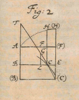
Figure 2. Leibniz’s diagram in the 1693 Acta Eruditorum. Courtesy of the Gottfried Wilhelm Leibniz Bibliothek-Niedersächsische Landesbibliothek- Hannover.

In this section I will contrast the geometrical proof of the fundamental theorem of the calculus given by Leibniz (Leibniz, 1693), (Kowalewski, 1908), (Struik 1969, 282) with the proof of this theorem given by Barrow discussed in the previous section. Leibniz started his formulation of this theorem with the statement

I shall now show that the general problem of quadratures can be reduced to the finding of a line [curve] that has a given law of tangency(declivitas), that is, for which the sides of the characteristic triangle have a given mutual relation. Then I shall show how this line [curve] can be described by a motion that I have invented. (Struik 1969, 282).

For his discussion Leibniz introduced a diagram, Fig. 2, that describes two curves $AH(H)$ and $C(C)$ with a common abscissa $AF$, and ordinates $HF$ and $FC$ respectively. Then Leibniz’s “general problem of quadratures” is to obtain the area bounded by the curve $AH(H)$ and the orthogonal lines $AF$, $HF$, by finding the curve $C(C)$ “that has a given law of tangency,” such that the ordinate $FC$ of this curve is proportional to this area. Leibniz wrote that he will “show how this line [$C(C)$] can be described by a motion that I have invented,” and the graphical device that he introduced for this purpose will be described in the next section.

The diagram associated with Leibniz’s geometrical construction, shown in Fig. 2, is essentially the same as Barrow’s diagram for Proposition 11, Lecture 10, shown in Fig. 1, except that Leibniz’s diagram is rotated with respect to Barrow’s diagram by $180^{o}$ around the horizontal axis $AF$. Thus, Leibniz’s curves $AH(H)$ and $C(C)$, Fig. 2, correspond to Barrow’s curves $ZEG^{\prime}$, and $AFI^{\prime}$, respectively.. Likewise, Leibniz’s tangent line $TGC$ to $C(C)$ corresponds to Barrow’s tangent line $TF$ to $AFI^{\prime}$, see Fig. 3. Moreover, I will show that Leibniz’s “tangency law” is the same as the relation, Eq. 3, applied by Barrow in his proof that $DT$ is the subtangent of $AFI^{\prime}$.

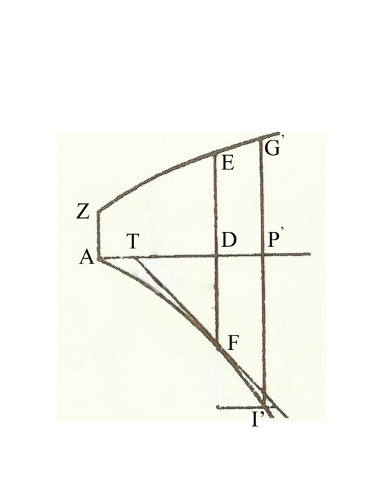
Figure 3. Barrow’s diagram, shown in Fig. 1, but rotated by $180^{0}$ around the horizonal $APD$ axis with some auxiliary lines deleted

Referring to his diagram, shown in Fig. 2, Leibniz continues

For this purpose I assume for every curve C(C’) a double characteristic triangle, one $TBC$, that is assignable, and one, $GLC$, that is inassignable, and these two are similar. The inassignable triangle consist of the parts $GL,LC$, with the elements of the coordinates $CF,CB$ as sides, and $GC$ the element of arc, as the base of the hypotenuse. But the assignable triangle $TBC$ consists of the axis, the ordinate, and the tangent, and therefore contains the angle between the direction of the curve (or its tangent) and the axis or base, that is, the inclination of the curve at a given point $C$. (Struik 1969, 283)

The tangent line to the curve $C(C)$ at $C$ is $TC$, and $GL$ and $GC$ are sides of its “characteristic triangle,” $GLC$, satisfying a “given mutual relation” specified below. But this triangle which Leibniz called inassignable , does not appear in the proof of Leibniz’s theorem, while another characteristic triangle, $CE\bar{C}$, where $\bar{C}$ (not indicated in Leibniz’s diagram, Fig. 2, is the intersection of the tangent line $TC$ with the extension of $(H)(F)$, turns out to be relevant to Leibniz’s proof. Leibniz formulated his “law of tangency” in terms of the sides $TB$ and $BC$ of the similar but assignable triangle $TBC$. The vertex $T$ of this triangle is the intersection of the tangent $TC$ with a line through the vertex $A$ of the curve $AH(H)$ perpendicular to the abscissa $AF$, and $B$ is the intersection with this line of a line from $C$ parallel to $AF$. In Proposition 11, Lecture 10, Barrow gave a proof of this law of tangency which he formulated, instead, in terms of the subtangent $T^{\prime}F$, where $T^{\prime}$ (not shown in Fig. 2) is the intersection of the tangent line $TC$ with the abscissa $AF$.

Up to this point, $C(C)$ has been treated as a given curve, but in the next sentence its construction is specified by the requirement that its slope conforms to what Leibniz, in his introduction, called a certain “law of tangency.”

Now let $F(H)$, the region of which the area has to be squared, be enclosed between the curve $H(H)$, the parallel lines $FH$ and $(F)(H)$, and the axis $F(F)$, on that axis let $A$ be a fixed point, and let a line $AB$, the conjugate axis, be drawn through $A$ perpendicular to $AF$. We assume that point $C$ lies on $HF$ (continued if neccesary); this gives a new curve $C(C)$ with the property that, if from point $C$ to the conjugate axis $AB$ [an axis through $A$ perpendicular to $AF$] (continued if neccesary) both its ordinate $CB$ (equal to $AF$) and tangent $CT$ are drawn, the part of the axis between them [$TB$] is to $BC$ as $HF$ to a constant $a$, or $a$ times $BT$ is equal to the rectangle $AFH$ (circumscribed about the trilinear figure $AFHA)$. (Struik 1969, 283)

At this stage the magnitude of $FC$, the ordinate of $C(C)$, was not specified, but further on Leibniz announced that $FC\cdot a$ is the area of the region $AHFA$, where $a$ is an arbitrary constant with dimensions of length. The relation that the curves $C(C)$ and $AH(H)$ must satisfy is the requirement

(11) $$\frac{TB}{BC}=\frac{HF}{a},$$

where $TB$ is the subtangent of $C(C)$ at $C$, and $HF$ is the corresponding ordinate of the curve $AH(H)$ at $F$. Presumably, this relation is Leibniz’s “ law of tangency” that Leibniz announced in his introduction. Leibniz, however, did not indicate the origin of this relation, but setting $TB/BC=E(C)/EC$ where $E(C)C$ is the associated characteristic triangle, it can be recognized as the fundamental theorem of the calculus that Leibniz had obtained in differential form, and Barrow had provedin Proposition 11, Lecture 10. But instead of giving a proof of this relation, in the next sentence Leibniz just asserted its validity:

This being established [the law of tangency, Eq. 11], I claim that the rectangle on $a$ and $E(C)$ (we must discriminate between the ordinates $FC$ and $(F)(C)$ of the curve) is equal to the region $F(H)$. (Struik 1969, 254)

By “the region $F(H)$” Leibniz meant the area bounded by the arc $H(H)$ of the curve $AFH$, the segment $F(F)$ of the abscissa, and the ordinates $HF$ and $(H)(F)$. From the exact similarity of the triangle $EC\bar{C}$ and the triangle $TBC$, where $\bar{C}$ (not indicate in Leibniz’s diagram, Fig. 2) is the intersection of the tangent line $TC$ with the extension of the of the ordinate $(H)(F)$, Fig. 2, it follows that

(12) $$\frac{E\bar{C}}{EC}=\frac{TB}{BC},$$

and substituting in this relation Leibniz’s form of the law of tangency, Eq. 11, yields

(13) $$a\cdot E\bar{C}=EC\cdot HF.$$

Since $CE=F(F)$, this expression is the area of the rectangle inscribed in the region $F(H)$, which is smaller that the area of this region. Hence

(14) $$E\bar{C}<E(C),$$

as is indicated in Leibniz’s diagram, Fig. 2, but in the limit that $EC$ becomes vanishingly small, the validity of Leibniz’s assertion, quoted above, is established. Then the approximation that $E(C)$ is the differential change in the ordinate of $C(C)$ for a change $EC$ in the abscissa, and $EC\cdot HF$, Eq. 13, is the differential area of the region $F(H)$, leads to the differential form of the fundamental theorem of the calculus along the same lines described by Barrow in Prop. 19, Lecture 11. As Leibniz explained it,

This follows immediately from our calculus. Let $AF=y,FH=z,BT=t$, and $FC=x$; then $t=zy/a$, according to our assumption [corresponding to Barrow’s law of tangency, Eq.2, in Leibniz’s coordinates]: on the other hand, $t=ydx/dy$ because of the property of the tangents expressed in our calculus. Hence $adx=zdy$ and therefore $ax=\int zdy=AFHA$.(Struik 1969, 284)

Here $dx=E(C)$ and $dy=F(F)=CE$. Therefore, $dx/dy=E(C)/EC$, $t/y=BT/AF$, and since triangles $TBC$ and $(C)EC$ are similar, $TB/AF=E(C)/EC$, which corresponds to $t=ydx/dy$. Here Leibniz invoked this relation for the subtangent $t$ as a “property of tangents expressed in our calculus,” but it can be seen to follow also from similarity relations between triangles in his diagram.

In summary, Leibniz based his 1693 geometrical proof of the fundamental theorem of the calculus on a “law of tangency”, Eq. 11, which originally he had developed in analytic form, but that also had been derived by Barrow in his Geometrical Lectures, Prop. 11, Lecture 10. He then proceed to demonstrate that a certain curve $C(C)$, constructed according to this law, gives the area bounded by a related curve $AH(H)$, along the same lines of Barrow’s proof of this theorem in Prop. 19, Lecture 11, using a diagram that turns out to be identical to Barrow’s diagram in Prop. 11, Lecture 10, after a $180^{0}$ rotation around the horizontal axis (see Fig. 3)

4. Leibniz graphical device to perform integrations

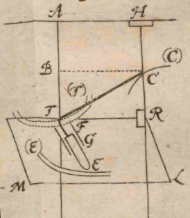
Figure 4. Leibniz’s diagram for a device to obtain graphically the area bounded by a given curve (1693 Acta Eruditorum). Courtesy of the Gottfried Wilhelm Leibniz Bibliothek-Niedersächsische Landesbibliothek- Hannover.

A novel feature of Leibniz’s 1693 discussion of the fundamental theorem of the calculus is his description of an ingenious graphical device to draw a curve $C(C)$ when its slope at each point is given. In his introduction, Leibniz mentioned that this curve “can be described by a motion I have invented” . The motivation for this device appears to have been a problem that was brought to his attention in 1676 by a physician, Claude Perrault, namely, to find the curve traced by a pocket watch pulled along a straight line by its chain Leibniz solved the problem, but he did not divulge his solution until about 20 years later (Bos 1988, 9).

In this section we provide an English translation of Leibniz’s description of his device, shown in Fig. 3, obtained from the German translation given in the Oswald’s Klassiker edition of the exact sciences (Kowalewski, 1908, 32), and we also give a brief discussion of the principles guiding its operation by an analytic description of the curves involved.

In Fig. 4, the right angle $TAH$ is fixed and lies on a horizontal plane. A vertical hollow cylinder $TG$, projecting out of this plane, can move along the side $AH$. On this cylinder another massive cylinder $FE$ slides upwards and downwards with a string $FTC$ attached at the tip $F$, in such a way that part $FT$ of the string lies inside the hollow cylinder and part $TC$ lies on the above mentioned horizontal plane. At the end $C$ of the string $TC$ there is a point (of a pen) that is lightly pressed against this plane to describes the curve $C(C)$. The movement comes from the hollow cylinder $TG$ that, while it is guided from $A$ along $AT$ it tightens $C$. The described point or pin $C$ pushes now $HR$ in the same horizontal plane at right angle to $AH$ (the other side of the fixed right angle $TAH$) towards $A$ in a progressive manner. This push does not prevent that the point $C$ is moved only by the pull of the string, and therefore follows its direction by this motion. There is also available a board $RLM$, that advances straight with the point $R$ perpendicularly along the staff $HR$, after all continuously driven by the hollow cylinder, so that $ATHR$ is a rectangle. Finally, there is a curve $E(E)$ described on this board (if you like in the form of a border) in which the massive cylinder by means of a cut that one can image at the end $E$, continuously intervenes; in this manner as $R$ moves towards $T$, the cylinder $FE$ moves upwards (along AT). Since the length $ET+TC$ is given (namely composed of the massive cylinder $EF$ and the entire string $FTC$), and given the relation between $TC$ and $R$ or $BC$ (from the given inclination [tangency] law), one obtains also the relation between $ET$and $TR$, the ordinate and abscissa of the curve $E(E)$ whose nature and description on the board $LRM$ can be obtained through ordinary geometry; one obtains also the description of the curve $C(C)$ through this available device. Now, however, it is in the nature of our motion, that $TC$ always is tangent to the curve $C(C)$ so the curve $C(C)$ is described with the given inclination law or the relation of the sides of the characteristic triangle $TRC$ or $TBC$. Since this curve is the squaring figure corresponding to the quadrature, as was shown a short while before, one has obtained the desired quadrature or measurement. (Kowalewski, 1908)

Given the slope of the curve $C(C)$, what is required to operate Leibniz’s device is the relation between the ordinate $ET$ and the abscissa $TR$ of the curve $E(E)$. Leibniz states, that this relation can be obtained “through ordinary geometry,” leaving it as an exercise for the reader. Given $CR$ and $TR$, the length $TC$ of the segment of the string lying on the plane $ATHR$ is

(15) $$TC=\sqrt{TR^{2}+CR^{2}},$$

and since the total length $TC+ET$ of the string has a fixed value $U$,

(16) $$ET=U-\sqrt{TR^{2}+CR^{2}}.$$

The operation of Leibniz’s integration device can also be understood by expressing its variable components, string length $TC$ and inclination or slope $CR/TR$, in analytic form. Introducing Cartesian coordinates $x,y,z$ along the mutually orthogonal axes $T_{o}R,T_{o}E,T_{o}A$ with origin at $T_{o}$, the initial location of the end point $T$ of the hollow cylinder, the curve $C(C)$ is described by the coordinates $x=TR$, $z=T_{o}B$, and the curve $E(E)$ by $x=TR$, $y=ET$. Then, by construction,

(17) $$\frac{dz}{dx}=\frac{CR}{TR},$$

(18) $$TC=x\sqrt{1+(\frac{dz}{dx})^{2}},$$

and

(19) $$y=U-x\sqrt{1+(\frac{dz}{dx})^{2}}.$$

For the special case that $ET$ is a constant,

(20) $$\frac{dz}{dx}=-\frac{\sqrt{a^{2}-x^{2}}}{x}$$

where $a=ET-U$, and the curve $C(C)$ is know as the $tractrix$.

5. Concluding remarks

In his translation of the early mathematical manuscripts of Leibniz, J. M. Child called attention to several instances where Leibniz’s discussion and diagrams are similar to those found in Barrow’s Geometrical Lectures (Child 1920). An example is discussed in Appendix A. But the relation of Leibniz’s 1693 geometrical proof of the fundamental theorem of the calculus to the corresponding proof of Barrow has not been analyzed before.

In his Geometrical Lectures, published in 1669, Barrow gave two elegant geometrical proofs of the fundamental theorem of the calculus discussed here in detail. In Proposition 11, Lecture 10, he established this theorem by rigorous geometrical bounds, while in Proposition 19, Lecture 11, he gave an alternate proof based on the application of infinitesimals along the lines practiced by mathematicians in the 17-th century. The eminent historian of science D.T. Whiteside, however, belittled Barrow’s proofs calling them “the work of a competent university don” (Whiteside 1961, 289), but this evaluation is contradicted by the evidence presented here. Likewise, another historian of science, M. S. Mahoney, concluded that Barrow “was not particularly original” (Mahoney 1990, 180,240), without, however, providing any evidence that Barrow’s proofs had been given earlier. Actually, Barrow was among the foremost mathematicians of his time, whose misfortune was to be eclipsed by his former protégé, Isaac Newton. In contrast to Whiteside’s and Mahoney’s remarks, a distinguished mathematician, Otto Toeplitz, concluded that “in a very large measure Barrow is indeed the real discoverer [of the fundamental theorem of the calculus] - insofar as an individual can ever be given credit within a course of development such as we have tried to trace here” (Toeplitz 1963, 98). After reviewing the historical record, M. Feingold also disagreed with Whiteside’s and Mahoney’s views (Feingold, 1990). Recently, Guicciardini discussed some of Barrow’s geometrical proofs showing that these proofs also had had a greater impact on Newton’s own contributions to the development of the calculus than had been realized in the past (Guicciardini, 2009). But Toeplitz also commented that “what Newton absorbed from the beginning remained foreign to Barrow throught his life: the turn from the geometrical to the computational function concept - the turn from the confines of the Greek art of proof to the easy flexibility of the indivisibles. On one page of his work Barrow alluded briefly to these matters, but quickly, as though in horror, he dropped them again.(Toeplitz 1963, 130)

Twenty three years after Barrow published his work, Leibniz presented a very similar geometrical proof of the fundamental theorem of the calculus theorem based on a “law of tangency” that Leibniz gave as “being established”. But this law corresponds to a theorem that Barrow had proved in Proposition 11, Lecture 10. Moreover, as has been shown here, Leibniz’s diagram, Fig. 2, is essentially the same, apart from orientation as Barrow’s diagram, Fig.1, given in this proposition, see also Fig. 3, and Leibniz’s arguments, which were based on differential quantities, are the same as those given by Barrow in Prop. 19, Lecture 11. Since Leibniz had obtained a copy of Barrow’s Geometrical Lecture in 1673, it is implausible that in the intervening twenty years he had never encountered Barrow’s two propositions, and the fact that his diagram and geometrical proof of the fundamental theorem of the calculus are virtually the same as Barrow’s is unlikely to be a coincidence. In fact, Leibniz’s marginal annotations in his copy of Barrow’s book indicate that at least by 1676 he had studied one of Barrow’s propositions contained in one of his last lectures, Prop. 1, Lecture 11 (Child 1920, 16) (Leibniz 2008, 301), see Appendix A. Child wrote that “as far as the actual invention of the calculus as he understood the term is concerned, Leibniz received no help from Newton or Barrow; but for the ideas that underlay it, he obtained from Barrow a great deal more than he acknowledged, and a very great deal less than he would have like to have got, or in fact would have got if only he would have been more fond of the geometry he disliked. For, although the Leibnizian calculus was at the time of this essay far superior to that of Barrow on the question of useful application, it was far inferior in the matter of completness.” (Child 1920, 136). Also Feingold commented that “I find it difficult to accept that historians can argue categorically that books that a person owned for years went unread simply because he or she failed failed to find dated notes from these books - especially when the figure in question is Leibniz, who was truly a voracious reader. And how can one determine with certainty what a genius like Leibniz was capable of comprehending from various books and letters he encounter or discussion he participated in, however confused their context appears to us today? Such reasoning, it seems to me, substitutes preconceived notion for constructive historical knowledge” (Feingold 1990, 331). Finally, it should not be forgotten that Leibniz’s, when composing his own version of planetary motion, Tentamen de motuum coelestium causis (Nauenberg 2010, 281), also denied having read Newton’s Principia, but his denial has been shown to be false (Bertoloni-Meli, 1993). Hence, Leibniz’s persistent claim, particularly during his priority controversy with Newton, of not having any indebtedness to Barrow in his development of the calculus, must be taken cum grano salis.

To his credit, in his 1693 article in the Acta Eruditorum, Leibniz also called attention to the usefulness of the fundamental theorem of the calculus for the evaluation of integrals, and for this purpose he designed a device to evaluate integrals graphically, see Section 4. Moreover, his work stimulated the applications of the calculus by his celebrated contemporaries, the Bernoulli brothers, Jacob Herman, and Pierre Varignon to the solution of problems in mechanics (Nauenberg, 2009). In his own development of the fundamental theorem of the calculus, Newton also realized the great usefulness of this theorem for integration, and for this purpose he created extensive tables of integrals. But he kept these results to himself, and he did not publish them until 1704 when he appended them to his $\it Opticks$ his Two Treatises on the Species and Magnitudes of Curvilinear Figures (Whiteside 1981, 131)

Finally, it should be emphasized that until the 19th century, when the analytic calculus was established on proper mathematical foundations, Barrow’s Prop. 10 Book 2 was already a rigorous proof, based on sound geometrical principles, of its fundamental theorem. Today, however, partly due to the dismissive remarks about Barrow by historians of science like Whiteside and Mahoney, (Whiteside 1961;Mahoney, 1990), it is Leibniz and Newton who get most of the credit for the development of the calculus while Barrow has been more or less forgotten. But, to quote Rosenberger,

Like all great advances in the sciences, the analysis of the infinitesimals did not suddenly arise, like Pallas Athena out of the head of Zeus, from the genius of a single author, but instead it was carefully prepared and slowly grown, and finally after laborious trials by the strength of genius, its general significance and long range meaning was brought to light” (Folkerts 2001, 299).

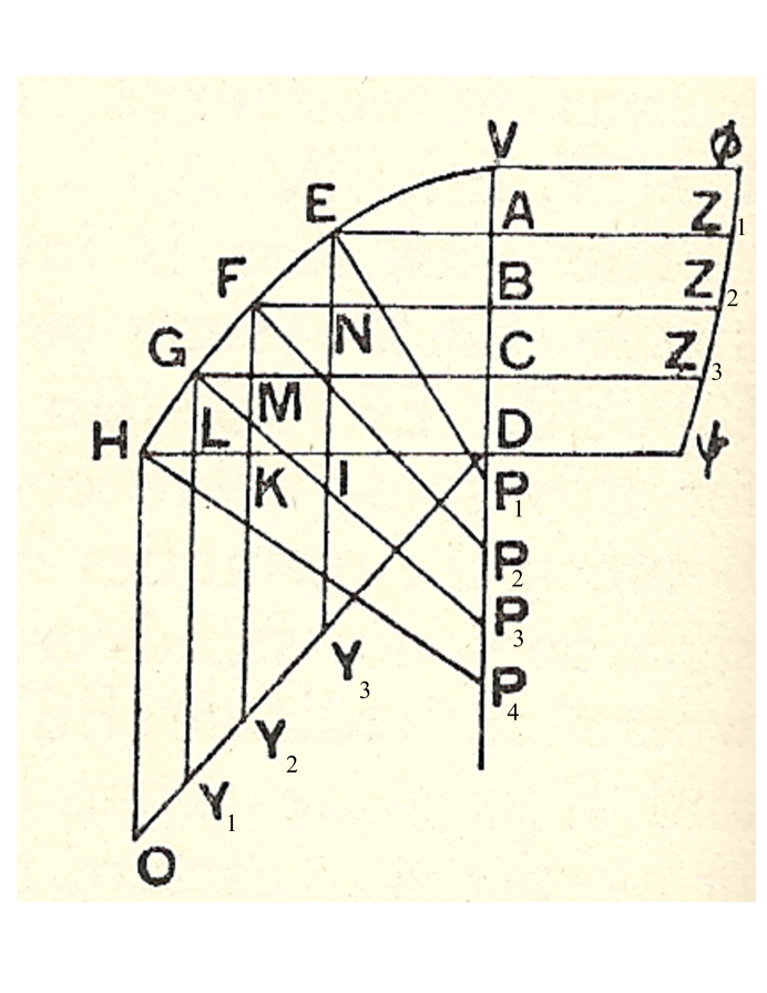
Figure 5. Barrow’s diagram for the integration of a curve of subnormals

Appendix A. Area of a curve of subnormals

In Proposition 1, Lecture 11, Barrow presented an ingenious geometrical construction to obtain the area bounded by a curve $\phi Z\psi$ with ordinates equal to the subnormals of a given curve $VEH$, with common abscissa $VD$, shown in Fig. 5. For clarity, we have added numerical subscript to the symbols $P,Z$ and $Y$ that appear repeatedly in Barrow’s original diagram. Barrow gave a proof that this area is equal to the area of a right angle isosceles triangle $HDO$ with sides equal to $HD$ shown at the bottom of his diagram, where $HD$ is the largest ordinate of $VEH$. The horizontal and vertical lines in Barrow’s diagram, Fig.5, illustrate his approximation by rectangles of the required areas, while the diagonal lines are the normals to $VEA$ at the chosen values of the abscissa of this curve. For example, at $A$ the subnormal $AP_{1}$ is obtained by finding the intersection at $P_{1}$ of the normal to $VEH$ at $E$ with the axis $VD$, where $EA$ is the ordinate $A$. The corresponding ordinate of $\phi Z\psi$ is constructed by setting $AZ_{1}=AP_{1}$, where $AZ_{1}$ is taken along the extension of $EA$. When $E$ approaches $V$, the arc $EV$ can be approximated by a straight line, and the “characteristic” triangle $VAE$, assumed to be infinitesimal, becomes similar to the triangle $EAP$. This construction is then repeated at the equally space points $B,C$ and $D$ along the abscissa $VD$, e.g. at the next point $B$ on the abscissa, the normal is $BP_{2}$, where this second value of $P$ is obtained by the intersection of the normal to $VED$ at $F$ with $VD$. In this case the characteristic triangle is $ENF$ which is similar to $FBP$, and $BZ_{2}=BP_{2}$. Then, in Barrow’s words,

the space $VD\psi\phi$ differs in the least degree only from the sum of the rectangles $DC\cdot D\psi+CB\cdot CZ_{3}+BA\cdot BZ_{2}+AV\cdot AZ_{1}$

Setting the intervals $AV,BA,CB,$ and $DC$ that appear to be equal as $\Delta x$, Barrow’s approximation to the area $VD\psi\phi$ is given by the area of the sum of rectangles, $\Delta x\cdot(AP_{1}+BP_{2}+CP_{3}+DP_{4})$. Then, in the limit that $\Delta x$ becomes vanishingly small, and the number of rectangles increases indefinitely, this sum becomes equal to the area $VD\psi\phi$ The similarity of the characteristic triangles with the triangles associated with the subnormals implies that $EA/VA=AP_{1}/EA,FN/EN=BP_{2}/FB,GM/FM=CP_{3}/CG$ and $HL/GL=DP_{4}/HD$. Hence, the sum $\Delta x\cdot(AP_{1}+BP_{2}+CP_{3}+DP_{4})=EA\cdot EA+FN\cdot FB+GM\cdot GC+HL\cdot HD$. According to Barrow’s construction, Fig. 5, the intervals $EA=ID,FN=KI,GM=LK$ and $HL$, are unequal, and $LY_{1}=GC,KY_{2}=FB$ and $IY_{3}=EA$. Hence, the above sum is equal to $HL\cdot HO+LK\cdot LY_{1}+KI\cdot KY_{2}+ID\cdot IY_{3}$ which corresponds to a sum of rectangles, giving an upper bound to the area of the right angle isosceles triangle $HDO$. In the limit that the interval $\Delta x$ become vanishingly small, and the number of rectangles that bound both areas increases indefinitely this sum gives the area of the triangle $HDO$, $(1/2)HD^{2}$, leading to Barrow’s conclusion that

(21) $$area\;VD\psi\phi=(1/2)HD^{2}$$

By always expressing position of points on his diagrams by letters, sometimes repeating the same letter for different points, Barrow lacked a suitable notation to describe his sums, particularly in the limit $n\rightarrow\infty$. Moreover, for this reason the relations that he had obtained geometrically between two finite sums was not evident algebraically

Although it lacked the rigorous mathematical justification of Barrow’s analysis, the power of Leibniz’s useful notation is that by the substitution of his relation $dx\cdot n(x)=dy\cdot y$ between the differentials $dx$ and $dy$, it reduces Barrow’s lengthy geometrical construction and derivation to a one line analytic relation between two integrals (Leibniz 1686)

(25) $$\int^{x}_{0}dx^{\prime}\;n(x^{\prime})=\int^{y}_{0}dy^{\prime}\;y^{\prime}=\frac{1}{2}y^{2}.$$

We have shown that Leibniz’s relation is based on the characteristic triangle discussed by Barrow, that gave rise to the relation $n_{i}/y_{i}\approx\Delta y_{i}/\Delta x$, for $i=1,n$ . Leibniz claimed that he first learned about the characteristic triangle from Pascal, but evidently he must have recognized it also when he examined Barrow’s diagram (Child 1920, 16).

Like Barrow, Leibniz also labelled points on his geometrical diagram with letters, but in the case that the same letter appeared repeated, he added a number of parenthesis corresponding to the number of times this letter was repeated, e.g. $C,(C),((C))$ etc. But later, he also distinguished repeated letters by adding a numerical subscript in front of these letter, e.g. ${}_{1}C,\;_{2}C,\;_{3}C$ (Child 1920,137; Leibniz 2008, 573; Bertoloni Meli 1993, 109,135)

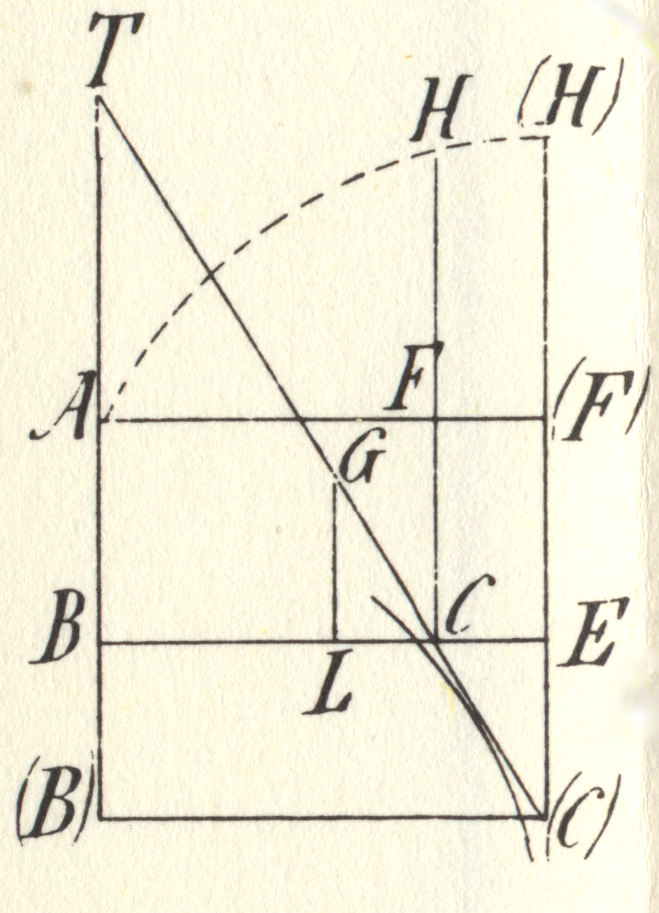
Figure 6. Reproduction of Leibniz’s 1693 diagram in Gerhardt’s edition of Leibniz’s mathematical papers (Leibniz, 1693)

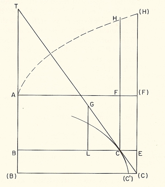
Figure 7. Reproduction of Leibniz’s 1693 diagram in (Struik 1696, 283)

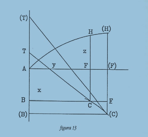
Figure 8. Reproduction of Leibniz’s 1693 diagram in (Giacardi 1995, 322)

Appendix B. Errors in the reproduction of Leibniz’s diagram

It should be pointed out that Leibniz 1693 diagram, Fig. 2, for his geometrical proof of the fundamental theorem of the calculus, has been repeatedly reproduced incorrectly.

In Gerhardt’s edition of Leibniz’s mathematical papers, this reproduction, shown in Fig. 5, contains two errors: 1) the curve labelled $C(C)$ touches tangentially the line $TC$ below the intersection $C$ of this line with $BE$, and 2) the extension of $TC$ ends at its intersection with the extension of $(F)(H)$, labelled incorrectly $(C)$. But $(C)$ is the end point of the curve $C(C)$, and the line $E(C)$ is proportional to the the area $FH(H)(F)$ which is greater than the distance between $E$ and the intersection of the extension of $TC$ that was labelled $\bar{C}$ in Section 2.

In Struik’s reproduction (Struik 1969, 283), shown in Fig. 6, Leibniz’s curve labelled $C(C^{\prime})$ is drawn correctly, but the intersection $(C)$ is again shown incorrectly as the extension of the tangent $TC$ intersecting the extension, of $(F)(H)$. Thus, when Struik translates Leibniz’s text

This being established, I claim that the rectangle of $a$ and $E(C)$ . . . is equal to the region $F(H)$.

it appears as if Leibniz had made a mistake here, but this is due to reference to Struik’s incorrect diagram.

More recently, L. Giacardi also reproduce Leibniz’s diagram incorrectly, see Fig 8, drawing the extension of the tangent line $TC$ of $C(C)$ at $C$ to intersect this curve at $(C)$, and by also introducing a line $T(C)$, supposedly tangent to $C(C)$ at $(C)$, which does not even appear in Leibniz’s diagram or in his text (Giacardi 1995, 322)

Such errors make Leibniz’s text difficult to comprehend.

6. Acknowlegdments

I would like to thank Niccolò Guicciardini for many helpful comments and discussions; Eberhard Knobloch and two anonymous referees for helpful criticisms of an earlier version of this manuscript, and for providing some relevant references. I also thank Mordechai Feingold for some helpful suggestions.

References

- [1] Baron, E.M., 1969. The Origins of the Infinitesimal Calculus (Pergamon Press)
- [2] Bertoloni Meli, D., 1993. Equivalence and Priority: Newton vs. Leibniz (Clarendon Press, Oxford)
- [3] Bos, H. J. M., 1973. Differentials, Higher-Order Differentials and the Derivative in the Leibnizian Calculus. Arch. Hist. Exact Sci. 14:1 90
- [4] Bos, H. J. M., 1986. Fundamental Concepts of the Leibnizian Calculus. 300 Jahre “Nova Methodus” von G. W. Leibniz (1684-1984). Symposion der Leibniz-Gesellschaft in Congresscentrum “Leewenhorst” in Noordwijkerhout (The Netherlands) 28 to 30 August 1984, edited by A. Heinekamp ( Franz Steiner Verlag Wiesbaden GMBH Suttgart )
- [5] Bos, H. J. M., 1988. Tractional Motion and the Legitimation of Transcendental Curves. Centaurus 31, 9-62.
- [6] Boyer, C. B., 1959. The History of the Calculus and its Conceptual Development. Dover Pub. New York.
- [7] Boyer, C. B., 1989. A History of Mathematics. (Wiley, New York)
- [8] Child, J. M., 1916. The Geometrical Lectures of Isaac Barrow. The Open Court Publishing Co.
- [9] Child, J. M., 1920. The Early Mathematical Manuscripts of Leibniz. Translated from the Latin texts published by Cal Immanuel Gerhardt with critical and historical notes. Merchant Books.
- [10] Child, J. M., 1930. Barrow, Newton and Leibniz, in their relation to the discovery of the calculus. Science progress in the twentieth century, XXV (London) pp. 295-307.
- [11] Feingold, M., 1990. Before Newton, the Life and Times of Isaac Barrow Cambridge Univ. Press.
- [12] Feingold, M., 1993. Newton, Leibniz and Barrow too, and attempt at a reinterpretation. Isis 84, 310-338.
- [13] Folkerts, M., Knobloch, E., and Reich, K. 2001. Infinitesimalmathematik Mass, Zahl und Gewicht, Mathematik als Schlüssel zu Weltverständnis und Weltbeherrschung. Wofenbüttel 300f.
- [14] Giacardi, L., 1995 Newton, Leibniz e il “Theorema fondamentalle” del calcolo integrale. Aspetti geometrici e aspetti algoritmici. In : Marco Panza and Clara Silvia roero (eds.): Geometria, flussioni e differenziali, Napoli, pp. 289-328.
- [15] Grabiner, J. V., 1981 The Origins of Cauchy’s Rigorous Calculus (The MIT Press, Cambridge)
- [16] Guicciardini, N., 2009. Isaac Newton on Mathematical Certainty and Method. MIT Press, Cambridge For a review, see Nauenberg, M., Notre Dame Philosophical Reviews, 2010, http://ndpr.nd.edu/review.cfm?id=20207.
- [17] van Heuraet, H., 1659. Epistola de transmutatione curvarum linearum in rectas. In: Geometria, Renato Des Cartes, Frans van Schooten’s Latin translation with commentaries.
- [18] Hofmann, J.E., 1974. Leibniz in Paris 1672-1676. Cambridge University Press.
- [19] Kowalewski, G., 1908. Über die Analyse des Undendlichen. In: Ostwald’s Klassiker der exakten Wissenschaftern Nr. 162, Engelann, Leipzig
- [20] Leibniz, G.W., 1693. Suplementum geometriae dimensioriae . . . , Acta Eruditorum , 385-392. Reproduced in Leibniz, Mathematische Schriften, band V, ed. Gerhardt, (Georg Olms verlag, Hildesheim, New York, 1971) pp. 294-301. English translation in Struik, D. J. 1969 A Source Book in Mathematics 1200-1800 Harvard Univ. Press, Cambridge, pp. 282- 284.
- [21] Leibniz, G.W., 1686. De geometriae recondita et analysi indivisibilium atque infinitorum, Acta Eruditorum 5. Reprinted in Leibniz, Mathematische Schriften, Abth. 2, Band III, 226-235. An English translation is given by Struik, D.J., A Source Book in Mathematics, 1200-1800, pp. 281, 282.
- [22] Leibniz, G.W.,2008. Sämtliche Schriften un Briefe, Herausgegeben von der Berlin-Brandenburgischen Akademie der Wissenchaften und der Akademie der Wissenschaften zu Göttingen. Siebente Reihe Mathematische Schriften. Fünfter Band. On line at http://www.leibniz-edition.de/Baende/ReiheVII.htm
- [23] Mahnke, D., 1926. Neue Einblicke in die Entdeckungsgeschichte der höheren Analysis, Abhandlungen der Preussischen Akademie der Wisssenschaften, phys-math klasse, Jahrgang 1925, Nr. 1 Berlin.
- [24] Mahoney, M. S., 1990. Barrow’s mathematics: between ancients and moderns, in Before Newton: The life and times of Isaac Barrow, edited by M. Feingold. Cambridge University Press, New York), pp. 179-249
- [25] Newton, I., 1960. The Correspondence of Isaac Newton Vol. 2 1676-1687, edited by H. W. Turnbull Cambridge University Press
- [26] Nauenberg, M., 2010. The early application of the calculus to the inverse square force problem. Archive for the History of Exact Sciences 64, 269-300.
- [27] Riemann, B., 1854. Ueber die Darstellbarkeit einer Function durch eine trigonometrische Reihe. Abhandlungen der K niglichen Gesellschaft der Wissenschaften zu G ttingen, vol. 13, 1867.
- [28] Struik, D. J., 1969. A Source Book in Mathematics, 1200 - 1800. Harvard University Press, Cambridge
- [29] Toeplitz, O., 1963. The Calculus, a genetic approach. University of Chicago Press M.I.T. Press, Cambridge, 2009.
- [30] Whiteside, D.T. 1961. Patterns of Mathematical Thought in the Later 17th Century. Archive for History of the Exact Sciences 179, 179-388.
- [31] Whiteside, D.T., 1981. The Mathematical Papers of Isaac Newton, Vol. VIII, 1697-1722 Cambridge University Press, Cambridge pp. 131-147.