Fast Distributed Computation of Distances in Networks

Abstract

This paper presents a distributed algorithm to simultaneously compute the diameter, radius and node eccentricity in all nodes of a synchronous network. Such topological information may be useful as input to configure other algorithms. Previous approaches have been modular, progressing in sequential phases using building blocks such as BFS tree construction, thus incurring longer executions than strictly required. We present an algorithm that, by timely propagation of available estimations, achieves a faster convergence to the correct values. We show local criteria for detecting convergence in each node. The algorithm avoids the creation of BFS trees and simply manipulates sets of node ids and hop counts. For the worst scenario of variable start times, each node $i$ with eccentricity $\mathop{\hbox{\rm ecc}}\nolimits(i)$ can compute: the node eccentricity in $\mathop{\hbox{\rm diam}}\nolimits(G)+\mathop{\hbox{\rm ecc}}\nolimits(i)+2$ rounds; the diameter in $2\mathop{\hbox{\rm diam}}\nolimits(G)+\mathop{\hbox{\rm ecc}}\nolimits(i)+2$ rounds; and the radius in $\mathop{\hbox{\rm diam}}\nolimits(G)+\mathop{\hbox{\rm ecc}}\nolimits(i)+2\mathop{\hbox{\rm radius}}\nolimits(G)$ rounds.

1 Introduction

This paper presents a distributed algorithm to simultaneously compute the diameter $D$, radius $R$ and node eccentricity $\mathop{\hbox{\rm ecc}}\nolimits(i)$ in all nodes of a network. An early knowledge of this topological information is useful since it is often used as input to other algorithms. For instance, the diameter or eccentricity can be used to simplify termination in leader election algorithms [8] and calibrate time-to-live parameters [7]; the radius and eccentricity allow determining center nodes [6], which are nice candidates to serve as coordinators in other distributed algorithms.

We assume a synchronous network model, while allowing variable start times, in which one or more nodes can start the algorithm with no prior coordination. The algorithm is designed to be fast in a precise sense; we are concerned with, not just asymptotic complexity, but exact bounds in the number of rounds.

The classic approach to this problem [8] is to compute the eccentricities by parallel construction of breadth first search (BFS) trees rooted at each node. Once eccentricities are known, each BFS tree can be reused to do a global computation, starting from the leafs and converging to each root node, allowing each to compute the maximum and minimum eccentricity (the network diameter $D$ and radius $R$). Considering a graph $G=(V,E)$, this classic approach has total message complexity of $\Theta(\left|V\right|\left|E\right|\log\left|V\right|)$ bits. The diameter and radius are known at all nodes in at most $4D+2$ rounds.

These time bounds can be improved if one departs from this modular multi-phase approach, where BFS trees are first constructed to compute eccentricities. This paper introduces an algorithm that propagates candidate values in a timely and continuous fashion, resulting in a faster convergence to the correct values. The challenge in this strategy is that a suitable termination method must be devised to detect, in each node, when the candidate values have converged. Under the same message complexity of the classic approach, the proposed algorithm reduces the number of rounds to compute the diameter to at most $3D+1$ rounds and the radius to at most $2D+2R$ rounds. To be more precise, with this algorithm each node $i$ with eccentricity $\mathop{\hbox{\rm ecc}}\nolimits(i)$ computes:

• the node eccentricity at most by round $\mathop{\hbox{\rm diam}}\nolimits(G)+\mathop{\hbox{\rm ecc}}\nolimits(i)+2$;

• the diameter at most by round $2\mathop{\hbox{\rm diam}}\nolimits(G)+\mathop{\hbox{\rm ecc}}\nolimits(i)+2$; and

• the radius at most by round $\mathop{\hbox{\rm diam}}\nolimits(G)+\mathop{\hbox{\rm ecc}}\nolimits(i)+2\mathop{\hbox{\rm radius}}\nolimits(G)$.

The paper is organized as follows. Section 2 presents the computing model and introduces notation. The algorithm is presented in Section 3. Example runs of the algorithm, proofs of local convergence criteria and global convergence bounds are also included in this section. The related work is discussed in Section 4, and the conclusions are presented in Section 5.

2 Network Model and Notation

We assume a synchronous network model, similar to the one described in [8]. The network is composed by a set of nodes connected by links, which we assume to be bidirectional; i.e., we have a simple, connected, unweighted, undirected graph $G=(V,E)$ with $\left|V\right|\geq 2$ nodes and $\left|E\right|\geq 1$ links. We assume globally unique identifiers for nodes, but no knowledge of the network topology or the number of nodes.

Computation proceeds in synchronous rounds. At each round, nodes first look at their state and compute what messages are sent, through a message-generation function; then nodes look at their state and messages received and compute the new state after the round, through a state-transition function. We assume no link or process failures. In order to obtain an asynchronous version of the algorithm a synchronizer $\alpha$ [1] can be used. We operate under a maximum bandwidth of $O(\left|V\right|\log\left|V\right|)$ bits, per link per round.

We assume the general case with variable start times. Nodes start as quiescent, a state in which they do not send messages nor transition to different states. Nodes wakeup when they receive a message from a special environment node (not part of $G$, connected to every node), or from an already active node.

We use $\mathop{\hbox{\rm d}}\nolimits(i,j)$ to denote the distance between nodes $i$ and $j$ (the length of the shortest path between nodes $i$ and $j$); $\mathop{\hbox{\rm ecc}}\nolimits(i)$ for the eccentricity of node $i$ (the maximum $\mathop{\hbox{\rm d}}\nolimits(i,j)$ between node $i$ and any other node $j$); $\mathop{\hbox{\rm diam}}\nolimits(G)$ for the network diameter (the maximum eccentricity over all nodes); $\mathop{\hbox{\rm radius}}\nolimits(G)$ for the network radius (the minimum eccentricity over all nodes); and $\mathop{\hbox{\rm nbrs}}\nolimits(i)$ for the set of neighbors of node $i$ (nodes connected to node $i$ by a link).

3 Algorithm

The algorithm is presented in Figure 1. At each round, a node $i$ sends the same message to all its neighbors (state variable $O_{i}$). A message is a non-empty set of tuples; the empty set represents absence of a message. The tuples in a message can be $\langle\textsc{bfs},\_,\_\rangle$, $\langle\textsc{diam},\_\rangle$ or $\langle\textsc{rad},\_\rangle$, where bfs, diam and rad are constants. Nodes do not need to distinguish between messages that arrive from different neighbors; the second parameter of the state-transition function (parameter $M_{i}$) is the set of messages received by node $i$ from all neighbors.

state variables:  $e_{i}$, node eccentricity, initially $e_{i}=0$

$d_{i}$, network diameter, initially $d_{i}=0$

$r_{i}$, network radius, initially $r_{i}=\infty$

$s_{i}$, status, initially $s_{i}=\textsc{quiescent}$

$I_{i}$, set of node ids, initially $I_{i}=\{\}$

$c_{i}$, consecutive rounds with no new BFS, initially $c_{i}=0$

$O_{i}$, message to be sent, initially $O_{i}=\{\}$

message-generation function:  $\mathop{\hbox{\rm msg}}\nolimits_{i}(\langle e_{i},d_{i},r_{i},s_{i},I_{i},c_{i},O_{i}\rangle,j)=O_{i}\qquad j\in\mathop{\hbox{\rm nbrs}}\nolimits(i)$

state-transition function:  $\mathop{\hbox{\rm trans}}\nolimits_{i}(\langle e_{i},d_{i},r_{i},s_{i},I_{i},c_{i},O_{i}\rangle,M_{i})=\langle e_{i}^{\prime},d_{i}^{\prime},r_{i}^{\prime},s_{i}^{\prime},I_{i}^{\prime},c_{i}^{\prime},O_{i}^{\prime}\rangle$ where $M=\bigcup\{m|m\in M_{i}\}$

if $s_{i}=\textsc{quiescent}\mathrel{\wedge}M=\{\}$ then  $\langle e_{i}^{\prime},d_{i}^{\prime},r_{i}^{\prime},s_{i}^{\prime},I_{i}^{\prime},c_{i}^{\prime},O_{i}^{\prime}\rangle=\langle e_{i},d_{i},r_{i},s_{i},I_{i},c_{i},O_{i}\rangle$ else  $M^{\prime}=\{\langle\textsc{bfs},j,h+1\rangle|\langle\textsc{bfs},j,h\rangle\in M,j\not\in I_{i}\}$

$M^{\prime\prime}=M^{\prime}\cup\{\langle\textsc{bfs},i,0\rangle|s_{i}=\textsc{quiescent}\}$

if $M^{\prime\prime}=\{\}$ then  $c_{i}^{\prime}=c_{i}+1$

else  $c_{i}^{\prime}=0$

  $e_{i}^{\prime}=\max(\{e_{i}\}\cup\{h|\langle\textsc{bfs},\_,h\rangle\in M^{\prime}\})$

$d_{i}^{\prime}=\max(\{d_{i}\}\cup\{d|\langle\textsc{diam},d\rangle\in M\}\cup\{e_{i}^{\prime}\})$

$r_{i}^{\prime}=\min(\{r_{i}\}\cup\{r|\langle\textsc{rad},r\rangle\in M\}\cup\{e_{i}^{\prime}|c_{i}^{\prime}=2\})$

$s_{i}^{\prime}=\textsc{active}$

$I_{i}^{\prime}=I_{i}\cup\{j|\langle\textsc{bfs},j,\_\rangle\in M^{\prime\prime}\}$

$M^{d}=\{\langle\textsc{diam},d_{i}^{\prime}\rangle|d_{i}^{\prime}>d_{i}\}$

$M^{r}=\{\langle\textsc{rad},r_{i}^{\prime}\rangle|r_{i}^{\prime}<r_{i}\}$

$O_{i}^{\prime}=M^{\prime\prime}\cup M^{d}\cup M^{r}$  

Figure 1: Algorithm.

Each node when awoken broadcasts a bfs message with its id and a hop counter, which starts at 0. Nodes keep the set of ids of all received bfs messages. When a node receives a bfs message from a node not yet known, it increments the hop counter and rebroadcasts it.

Nodes know their eccentricity is at least the largest hop count received in a bfs message, which they keep in a variable ($e_{i})$. Nodes also keep in two other variables ($d_{i}$, $r_{i}$) a lower bound estimate for the diameter and an upper bound estimate for the radius. When a node increases the diameter estimate; it broadcasts a diam message with the new value. A node increases its diameter value when (1) its eccentricity surpasses its diameter estimate or (2) it receives a diam message whose value is higher that its diameter value. Estimation of the radius is also driven by eccentricity, but must be deferred until each node detects its correct eccentricity. When that happens, and also when a lower estimate for the radius is received, a rad message is broadcast.

It is easy to see that at some point every node will have awakened; later everyone will have received a bfs from everyone else and will have their eccentricity stored in the respective variable; and later still nodes will receive some diam message with the network diameter, originating from some maximum eccentricity node (a periphery node). Similarly, a rad message originating from a minimum eccentricity node (a center node) will arrive eventually at all nodes.

The relevant question is convergence detection, i.e., when will nodes know that their eccentricity, diameter and radius variables have converged to the correct values. For this purpose, and inspired by the approach in [9], nodes have a variable which stores the number of consecutive rounds for which no new bfs messages arrived. Later, we will show how this variable can be used for convergence detection.

In order to analyze the communication complexity of the whole execution of the algorithm, we can first observe that each bfs message can be encoded in $\Theta(\log\left|V\right|)$ bits, since its dominated by the size of the ids. Each node retransmits exactly one bfs message for every other node, totaling $\Theta(\left|V\right|\left|E\right|\log\left|V\right|)$ bits. Since the diameter can only increase at most $D$ times, each node broadcasts at most $D$ diam messages, totaling $O(D\left|E\right|\log D)$ bits. Similarly for rad messages. Thus, total message complexity is $\Theta(\left|V\right|\left|E\right|\log\left|V\right|)$ bits.

3.1 Example Runs

Prior to the formal proofs of the algorithm properties, we now convey some intuition by illustrating its execution in two different graphs. The first graph is a path with eleven nodes, depicted in Figure 2. Nodes 0 and 10 and are the only two nodes in the periphery, thus defining the diameter; node 5 is the single node in the graph center. We consider a run where node 0 is activated and we will observe how the local variables evolve in nodes 0, 5 and 10 (Figures 3, 4 and 5, respectively).

Figure 2: Path graph.

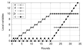
Figure 3: Path graph, start at 0, probing at node 0.

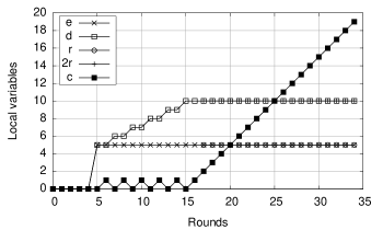
Figure 4: Path graph, start at 0, probing at node 5.

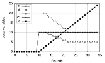
Figure 5: Path graph, start at 0, probing at node 10.

When probing the variables at node 0 we can observe that each two rounds a new bfs is received until bfs messages from all nodes have arrived. Each time a new bfs is received the $c_{i}$ counter is reset. Thus, when $c_{i}$ reaches two the node knows that its eccentricity variable $e_{i}$ has reached the correct final value. This happens in nodes 0, 5 and 10 at rounds 22, 17 and 22, respectively.

Once eccentricity is stabilized nodes start disseminating rad messages in order to detect the minimum eccentricity. Since local radius estimates can only decrease, one must establish a termination condition so that each node knows that it reached the correct radius. We will show that this is safely achieved when $c_{i}\geq 2r_{i}$. The run in Figure 5 shows that no sooner than this has the radius reached its final value of 5 in node 10.

Diameter dissemination, via diam messages, starts even if nodes are still updating their (monotonically increasing) estimates for eccentricity. For instance, in Figure 4 we see that node 5 is activated at round 5 (receiving bfs messages from nodes 0 to 4) and sets both $e_{i}$ and $d_{i}$ to 5 (its received hop distance from node 0, the furthest away). As nodes 6 to 10 are activated, in the next rounds, the diameter estimate $d_{i}$ at node 5 gets updated each two rounds. We will show that in order for a node to know that the diameter has reached its final value it needs to locally observe that $c_{i}\geq 2$ and $c_{i}>d_{i}$. This happens in nodes 0, 5 and 10 at rounds 31, 26 and 21, respectively. One can notice that in this path graph the diameter is stable even before those rounds.

However, it is easy to construct a T shaped graph where detection cannot occur before the mentioned round. In Figure 6 we show such a graph. Here, a critical case happens when a node not in a diameter defining path (for example, node 14) is the first to be activated. As seen in Figure 7 this leads to a run where the diameter estimation seems to be stable for a large number of rounds (between round 18 and 27), finally increases at round 28, with convergence being detected only when $c_{i}>d_{i}$ at round 29. In the next section we prove that these convergence criteria are correct for general graphs.

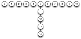
Figure 6: T shaped graph.

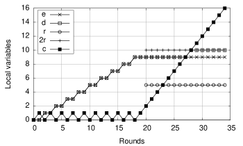
Figure 7: T shaped graph, start at 14, probing at node 14.

3.2 Local Convergence Criteria

We now establish results that allow a node to know, using local information, that the variables estimating node eccentricity, network diameter and network radius have converged to the correct values. In the following we will use $i$, $j$, $u$, and $v$ to range over node ids and $r$, $n$ and $k$ to range over non-negative integers.

Definition 3.1.

$A_{i}(r)\doteq\{j|\mathop{\hbox{\rm d}}\nolimits(i,j)\leq r\mathrel{\wedge}s_{j}(r-\mathop{\hbox{\rm d}}\nolimits(i,j))=\textsc{active}\}.$

$A_{i}(r)$ denotes the “area of visibility” of node $i$ after round $r$: the set of nodes whose bfs messages arrive at $i$ no later than round $r$. It is easy to see that $A_{i}$ is monotonic: $A_{i}(r)\subseteq A_{i}(r+1)$.

Lemma 3.1.

After any round $r$, $I_{i}(r)=A_{i}(r)$.

Proof.

If $j\in I_{i}(r)$ then $i$ must have received no later than round $r$ a bfs message starting at $j$; it traveled $\mathop{\hbox{\rm d}}\nolimits(i,j)$ hops, which means that $\mathop{\hbox{\rm d}}\nolimits(i,j)\leq r$ and $j$ was active after round $r-\mathop{\hbox{\rm d}}\nolimits(i,j)$; therefore $j\in A_{i}(r)$. If $j\in A_{i}(r)$, then $\mathop{\hbox{\rm d}}\nolimits(i,j)\leq r$ and $j$ was active after round $r-\mathop{\hbox{\rm d}}\nolimits(i,j)$. This implies that $j$’s bfs message arrives at $i$ not later than round $r$; therefore, $j\in I_{i}(r)$. ∎

Lemma 3.2.

If $c_{i}(r+2)\geq 2$, then $A_{i}(r)=V$.

Proof.

If $A_{i}(r)\neq V$ then there are two nodes, $u\in A_{i}(r)$ and $v\not\in A_{i}(r)$ which are adjacent, i.e., $\mathop{\hbox{\rm d}}\nolimits(u,v)=1$. This means that $s_{u}(r-\mathop{\hbox{\rm d}}\nolimits(i,u))=\textsc{active}$ and $s_{v}(r-\mathop{\hbox{\rm d}}\nolimits(i,v))=\textsc{quiescent}$. Since $u$ and $v$ are adjacent, then $s_{v}(r+1-d(i,u))=\textsc{active}$. There are three possible cases: (1) $\mathop{\hbox{\rm d}}\nolimits(i,u)=\mathop{\hbox{\rm d}}\nolimits(i,v)$, in which case $v$ became active in round $r+1-\mathop{\hbox{\rm d}}\nolimits(i,v)$, and $i$ receives the bfs from $v$ at round $r+1$; (2) $\mathop{\hbox{\rm d}}\nolimits(i,v)=\mathop{\hbox{\rm d}}\nolimits(i,u)+1$, in which case $s_{v}(r+2-\mathop{\hbox{\rm d}}\nolimits(i,v))=\textsc{active}$, and $i$ receives the bfs from $v$ at either round $r+1$ or round $r+2$; (3) $\mathop{\hbox{\rm d}}\nolimits(i,v)=\mathop{\hbox{\rm d}}\nolimits(i,u)-1$, cannot happen, as it contradicts $s_{v}(r-\mathop{\hbox{\rm d}}\nolimits(i,v))=\textsc{quiescent}$. In any case, $c_{i}(r+1)=0$ or $c_{i}(r+2)=0$. Therefore, since $c_{i}$ can only increase 1 unit per round, it follows that if $c_{i}(r+2)\geq 2$, then $A_{i}(r)=V$. ∎

Lemma 3.3.

After any round $r$, $e_{i}(r)=\max(\{0\}\cup\{\mathop{\hbox{\rm d}}\nolimits(i,j)|j\in I_{i}(r)\})$.

Proof.

Trivial induction on the number of rounds. ∎

Theorem 3.1 (eccentricity convergence).

If $c_{i}(r+2)\geq 2$, then $e_{i}(r)=\mathop{\hbox{\rm ecc}}\nolimits(i)$.

Proof.

Combine the previous three lemmas. ∎

Lemma 3.4.

If for some $r$ and $n\geq 2$, $c_{i}(r+n)=n$, then for all $k$, $c_{i}(r+k)=k$.

Proof.

After the first round $r$ such that $c_{i}(r+2)=2$, by the first two lemmas $I_{i}(r)=V$. This implies that for $r^{\prime}\geq r$, $c_{i}(r^{\prime}+1)=c_{i}(r^{\prime})+1$. ∎

Theorem 3.2 (diameter convergence).

When $c_{i}(r)\geq 2$ and $c_{i}(r)>d_{i}(r)$, then $d_{i}(r)=\mathop{\hbox{\rm diam}}\nolimits(G)$.

Proof.

By contradiction. Assume $c_{i}(r)\geq 2$ and $c_{i}(r)>d_{i}(r)$ but $d_{i}(r)<\mathop{\hbox{\rm diam}}\nolimits(G)$. By Theorem 3.1, $e_{i}(r)=\mathop{\hbox{\rm ecc}}\nolimits(i)$. Also, it is trivial that $d_{i}(r)\geq e_{i}(r)$. Then, as in a graph all the eccentricities between the radius and the diameter are present [3], there exists two nodes $u$ and $v$ with $\mathop{\hbox{\rm d}}\nolimits(u,v)=d_{i}(r)+1$. Assume without loss of generality that $\mathop{\hbox{\rm d}}\nolimits(i,u)\geq\mathop{\hbox{\rm d}}\nolimits(i,v)$. From the previous lemma, for $r^{\prime}=r-c_{i}(r)$, it follows that $c_{i}(r^{\prime}+k)=k$. As $c_{i}(r^{\prime}+2)=2$, by Lemma 3.2, $A_{i}(r^{\prime})=V$; therefore $s_{u}(r^{\prime}-\mathop{\hbox{\rm d}}\nolimits(i,u))=\textsc{active}$. Then, $d_{v}(r^{\prime}-\mathop{\hbox{\rm d}}\nolimits(i,u)+\mathop{\hbox{\rm d}}\nolimits(u,v))\geq\mathop{\hbox{\rm d}}\nolimits(u,v)$ (bfs from $u$ has reached $v$). Furthermore, $d_{i}(r^{\prime}-\mathop{\hbox{\rm d}}\nolimits(i,u)+\mathop{\hbox{\rm d}}\nolimits(u,v)+\mathop{\hbox{\rm d}}\nolimits(i,v))\geq\mathop{\hbox{\rm d}}\nolimits(u,v)$ (diam message from $v$ has reached $i$). Since $\mathop{\hbox{\rm d}}\nolimits(i,u)\geq\mathop{\hbox{\rm d}}\nolimits(i,v)$, then $d_{i}(r^{\prime}+\mathop{\hbox{\rm d}}\nolimits(u,v))\geq\mathop{\hbox{\rm d}}\nolimits(u,v)$. Recall that $\mathop{\hbox{\rm d}}\nolimits(u,v)=d_{i}(r)+1$, and let $r^{\prime\prime}=r^{\prime}+\mathop{\hbox{\rm d}}\nolimits(u,v)=r-c_{i}(r)+d_{i}(r)+1$. From the assumption $c_{i}(r)>d_{i}(r)$, it means that $r^{\prime\prime}\leq r$, which together with $d_{i}(r^{\prime\prime})\geq d_{i}(r)+1$ contradicts the monotonicity of $d_{i}$. ∎

Theorem 3.3 (radius convergence).

When $c_{i}(r)\geq 2r_{i}(r)$, then $r_{i}(r)=\mathop{\hbox{\rm radius}}\nolimits(G)$.

Proof.

We assume networks with at least one link and two nodes, which means $r_{i}(r)\geq 1$. If $c_{i}(r)\geq 2r_{i}(r)$, we have $c_{i}(r)\geq 2$, which means that, from Lemma 3.4, all bfss have already reached node $i$ after round $r^{\prime}=r-c_{i}(r)$, and from $r^{\prime}$ on we have $c_{i}(r^{\prime}+k)=k$. Assume, by contradiction, that $r_{i}(r)>\mathop{\hbox{\rm radius}}\nolimits(G)$. Then, at most after round $r^{\prime}+r_{i}(r)-1$, all bfss have reached some node $u$ in the center of the network. At most two rounds later, after round $r^{\prime\prime}=r^{\prime}+r_{i}(r)+1$, we have $c_{u}(r^{\prime\prime})\geq 2$ and $u$ has sent a rad message with the network radius. At most $r_{i}(r)-1$ rounds later, after round $r^{\prime\prime\prime}=r^{\prime}+2r_{i}(r)$ this message arrives at $i$ and $r_{i}(r^{\prime\prime\prime})=\mathop{\hbox{\rm radius}}\nolimits(G)$. But assuming $c_{i}(r)\geq 2r_{i}(r)$ it means that $r^{\prime\prime\prime}\leq r$, which contradicts $r_{i}$ being monotonically decreasing. As $r_{i}$ results from some eccentricity and is always an upper bound of the radius, we must have $r_{i}(r)=\mathop{\hbox{\rm radius}}\nolimits(G)$. ∎

3.3 Convergence Bounds

We now determine upper bounds on the number of rounds for convergence of eccentricity, diameter and radius. Given that we have described the algorithm for the general case of variable starting times, what matters is the number of rounds after the first activation; i.e., ignoring an initial sequence of rounds with all nodes inactive. Therefore, in this section we consider that the first node became active after round 0; round 1 is when the first non-environment message is sent.

Proposition 3.1 (eccentricity bound).

Node $i$ can determine its eccentricity at most in $\mathop{\hbox{\rm diam}}\nolimits(G)+\mathop{\hbox{\rm ecc}}\nolimits(i)+2$ rounds.

Proof.

After round $\mathop{\hbox{\rm diam}}\nolimits(G)$ all nodes are active, so the last bfs arrives at $i$ at most after round $\mathop{\hbox{\rm diam}}\nolimits(G)+\mathop{\hbox{\rm ecc}}\nolimits(i)$. Two rounds later the $c_{i}$ variable reaches $2$ and from Lemma 3.1 the eccentricity has already converged. ∎

Proposition 3.2 (diameter bound).

Node $i$ can determine the network diameter at most in $2\mathop{\hbox{\rm diam}}\nolimits(G)+\mathop{\hbox{\rm ecc}}\nolimits(i)+1$ rounds.

Proof.

After round $\mathop{\hbox{\rm diam}}\nolimits(G)$ all nodes are active, so the last bfs arrives at $i$ at most after round $\mathop{\hbox{\rm diam}}\nolimits(G)+\mathop{\hbox{\rm ecc}}\nolimits(i)$. Subsequently $c_{i}$ starts increasing and after further $\mathop{\hbox{\rm diam}}\nolimits(G)+1$ rounds the local condition $c_{i}>d_{i}$ is met. As we are considering networks with at least one link, i.e., $\mathop{\hbox{\rm diam}}\nolimits(G)\geq 1$, then at this round we have also $c_{i}\geq 2$ and from Theorem 3.2 the diameter has converged. ∎

Proposition 3.3 (radius bound).

Node $i$ can determine the network radius at most in $\mathop{\hbox{\rm diam}}\nolimits(G)+\mathop{\hbox{\rm ecc}}\nolimits(i)+2\mathop{\hbox{\rm radius}}\nolimits(G)$ rounds.

Proof.

After round $\mathop{\hbox{\rm diam}}\nolimits(G)$ all nodes are active, so the last bfs arrives at $i$ at most after round $\mathop{\hbox{\rm diam}}\nolimits(G)+\mathop{\hbox{\rm ecc}}\nolimits(i)$; afterwards $c_{i}$ starts increasing and after round $r=\mathop{\hbox{\rm diam}}\nolimits(G)+\mathop{\hbox{\rm ecc}}\nolimits(i)+2\mathop{\hbox{\rm radius}}\nolimits(G)$ we have $c_{i}(r)\geq 2\mathop{\hbox{\rm radius}}\nolimits(G)$. Also, after at most round $\mathop{\hbox{\rm diam}}\nolimits(G)+\mathop{\hbox{\rm radius}}\nolimits(G)$ all bfs have arrived at all center nodes; two rounds later, at most after round $r^{\prime}=\mathop{\hbox{\rm diam}}\nolimits(G)+\mathop{\hbox{\rm radius}}\nolimits(G)+2$, each center node sends a rad message containing $\mathop{\hbox{\rm radius}}\nolimits(G)$. There are two possibilities: (1) $\mathop{\hbox{\rm ecc}}\nolimits(i)>1$, the rad message from a center node $j$ arrives at $i$ at most $\mathop{\hbox{\rm radius}}\nolimits(G)$ rounds later, which means that at most after round $r^{\prime\prime}=\mathop{\hbox{\rm diam}}\nolimits(G)+2\mathop{\hbox{\rm radius}}\nolimits(G)+2$ we have $r_{i}(r^{\prime\prime})=\mathop{\hbox{\rm radius}}\nolimits(G)$; given that $r^{\prime\prime}\leq r$, then $r_{i}(r)=\mathop{\hbox{\rm radius}}\nolimits(G)$, and the local radius convergence criteria $c_{i}(r)\geq 2r_{i}(r)$ is met; (2) $\mathop{\hbox{\rm ecc}}\nolimits(i)=1$, in which case $\mathop{\hbox{\rm radius}}\nolimits(G)=1$, $i$ is a center node, and at round $r^{\prime}$ we have $r_{i}(r^{\prime})=\mathop{\hbox{\rm radius}}\nolimits(G)$; as in this case $r^{\prime}=r$, we have $c_{i}(r)\geq 2r_{i}(r)$ as well. ∎

Corollary 3.1.

All nodes know: their eccentricity at most in $2D+2$ rounds; the diameter at most in $3D+1$ rounds; and the radius at most in $2D+2R$ rounds.

3.4 Termination

To keep the presentation clear and avoid cluttering, we did not include in the algorithm the mechanics of termination; i.e., each node reaching a “terminated” state in which it stops sending messages. In general distributed termination is independent from reaching some result, and nodes may have to keep propagating messages for some time.

In this case, however, it is easy to see that when a node has determined both the radius and diameter through the local convergence criteria, all neighbors will have the same criteria met after at most one more round. (After one more round, each node $j$ neighbor from $i$, will have $c_{j}$ with at least the same value node $c_{i}$ had, and both $r_{j}$ and $d_{j}$ will have the same values as in node $i$.) Therefore, after having met both criteria for radius and diameter, a node needs only execute one more round and stop.

3.5 Improving Storage Requirements

In the previously described algorithm each node accumulates in the $I$ variable all ids received in all previous rounds. Although it has made the description intuitive and streamlined proofs, it means that, regardless of network topology, by the end of the execution each node will need to store $\Theta(\left|V\right|)$ ids.

Here we show that it is enough to keep in the state only the ids received in the two previous rounds. While this modification does not change the worst case space requirement complexity (it still remains $O(\left|V\right|)$ ids for general graphs and uncoordinated start times), it may be useful in practice. As an example, for 2D geometrical networks (e.g. a geographically spread sensor network with links according to inter-node distance), under synchronized start times, the number of ids that arrive in a single round (and need to be stored) will be $O(\sqrt{\left|V\right|})$. Notice that these specific configurations also reduce the required channel bandwidth, and that in other specific graph topologies, these uppers bounds on stored state can be even more tight.

The modification to the algorithm is trivial and consists of replacing state variable $I$ by a pair $I,J$ used as a sliding window; replacing the test $j\not\in I_{i}$ with $j\not\in I_{i}\cup J_{i}$ and replacing $I_{i}^{\prime}=I_{i}\cup\{j|\langle\textsc{bfs},j,\_\rangle\in M^{\prime\prime}\}$ with $I_{i}^{\prime}=J_{i}$ and $J_{i}^{\prime}=\{j|\langle\textsc{bfs},j,\_\rangle\in M^{\prime\prime}\}$. The modification is possible due to the following property of the original algorithm.

Proposition 3.4.

A node $j$ can only receive BFS messages $\langle\textsc{bfs},i,\_\rangle$, originated in a node $i$ activated at round $r$, in rounds $r+\mathop{\hbox{\rm d}}\nolimits(i,j)$, $r+\mathop{\hbox{\rm d}}\nolimits(i,j)+1$ and $r+\mathop{\hbox{\rm d}}\nolimits(i,j)+2$.

Proof.

The first round, where node $j$ can receive a $\langle\textsc{bfs},i,\_\rangle$ message, is $r^{\prime}=r+\mathop{\hbox{\rm d}}\nolimits(i,j)$, by the shortest path from $i$; $j$ rebroadcasts it and at round $r^{\prime}+1$ it arrives at all neighbors, if any. Also at round $r^{\prime}+1$ node $j$ may receive such a message if there exists a neighbor node $u$ at the same distance from $i$ (i.e., $\mathop{\hbox{\rm d}}\nolimits(i,u)=\mathop{\hbox{\rm d}}\nolimits(i,j)$); this neighbor, similarly to $j$, has received such a message at round $r^{\prime}$ and has rebroadcasted it. At round $r^{\prime}+2$ node $j$ can receive such a message if it has a neighbor $u$ one hop further away from $i$ (i.e., $\mathop{\hbox{\rm d}}\nolimits(i,u)=\mathop{\hbox{\rm d}}\nolimits(i,j)+1$); this neighbor has received the message at round $r^{\prime}+1$ and has rebroadcasted it at round $r^{\prime}+2$. Because any neighbor $u$ of $j$ has stored $i$ in the respective $I_{u}$ variable after at most round $r^{\prime}+1$, it will not rebroadcast any $\langle\textsc{bfs},i,\_\rangle$ message in any round later than $r^{\prime}+2$, from which such messages cannot reach $j$ later than round $r^{\prime}+2$. ∎

4 Related Work

As mentioned in the introduction, our algorithm improves the classic modular approach [8], where BFS trees are first computed at each node and later reused to perform a global computation of the network radius and diameter (in at most $4D+2$ rounds). By Corollary 3.1, we achieve a speedup of $D$ rounds for computing the diameter, and since $D\leq 2R\leq 2D$ the speedup for computing the radius varies between $2$ and $D+2$ rounds. The maximum speedup occurs, for example, in path graphs. This improvement is achieved with the same message complexity of $\Theta(\left|V\right|\left|E\right|\log\left|V\right|)$ bits, and the same space complexity of $O(\left|V\right|)$ ids and computation complexity per round of $O({\left|V\right|}^{2})$ at each node.

The work in [10] computes the diameter under the more restrictive synchronized start time model, where all nodes are activated at the first round. This is a fast algorithm since they also disseminate candidate values for eccentricities before they converge. However, since they assume that all nodes are active in the first round the local termination criteria is much simpler. When restricted to a setting where all nodes are active in the first round our algorithm outputs the diameter in the same time bound. Even though we are more general, we have significant improvements in message and space complexity.

Related to the computation of the radius and the eccentricity is finding the network center. To the best of our knowledge, within similar bounds for space and processing complexity per round, the fastest algorithm so far to find network center nodes was proposed by Korach, Rotem and Santoro [6]. This algorithm builds on a simpler algorithm to find a center of a tree, and the observation that the center of a general network must also be the center of its own BFS tree: the initiator node triggers BFS generation at all nodes, picks a center among all candidates which are centers of their own BFS, and later disseminates this information to all nodes. The closest center node $c$ to the initiator node $i$ will receive the confirmation that it is indeed a center of the network by round $4\mathop{\hbox{\rm radius}}\nolimits(G)+\mathop{\hbox{\rm d}}\nolimits(i,c)+1$, with total message complexity of $\Theta(\left|V\right|\left|E\right|\log\left|V\right|)$ bits. Notice that, in contrast to this, our algorithm is fully symmetrical, not requiring a distinguished node as initiator (which would have to be chosen in some way, e.g. by a leader election). Even discounting this factor, our more general algorithm has no time penalty: in fact, it can be shown that it even improves this upper bound by at least one round.

A more general problem than computing the eccentricities, radius and diameter is that of computing the distance matrix or all-pairs shortest path matrix in a network. In fact, relying on this connection, a faster distributed variant of our algorithm could be designed to compute the radius and diameter: instead of propagating just the distances, each node propagates sets of neighbors – at most by round $2\mathop{\hbox{\rm diam}}\nolimits(G)+2$ all nodes would be able to determine the full topology of the network and run a standard unweighted all-pairs shortest path algorithm with computation complexity $O(\left|V\right|\left|E\right|)$ at the last round. Unfortunately, even assuming that computation complexity per round is negligible, this algorithm requires $\Theta({\left|V\right|}^{2})$ space complexity at each node, which is impractical for large networks. Moreover the message complexity increases to $\Theta({\left|E\right|}^{2}\log\left|V\right|)$ bits, and requires a bandwidth of $O(\left|E\right|\log\left|V\right|)$ bits per link.

With such large bandwidth it is possible to decrease the message complexity using more elaborated approaches. For example, Kanchi and Vineyard [5] propose a distributed algorithm to compute the all-pairs shortest path matrix with message complexity of $O(\left|V\right|\left|E\right|\log\left|V\right|)$ bits: a spanning tree is first computed using the algorithm proposed by Awerbuch [2] and later reused to propagate the topological information to a root node that computes the distance matrix and disseminates it to all nodes. The tradeoff for this optimization is, unfortunately, a substantial increase in the number of rounds, although still $O(\left|V\right|)$.

Message complexity can also be reduced by trading off accuracy. For example, Gu and Cheng [4] propose a distributed algorithm to compute an estimate $\hat{\mathop{\hbox{\rm diam}}\nolimits(G)}$ for the diameter, such that $\mathop{\hbox{\rm diam}}\nolimits(G)\leq\hat{\mathop{\hbox{\rm diam}}\nolimits(G)}\leq\mathop{\hbox{\rm diam}}\nolimits(G)+2$. Unfortunately, the bandwidth requirements are slightly worse than ours and the improvement in message complexity does not extend to time complexity: although the authors do not quantify this measure, it is clear from the algorithm presentation that the number of rounds until completion is substantially larger than ours. Moreover, this algorithm also requires a distinguished node as initiator.

5 Conclusions

In this paper we propose a time efficient algorithm that computes in all nodes of a network the values of the node eccentricity, and the network diameter and radius. The algorithm is very flexible in the sense that it does not require a distinguished node, one or more nodes can initiate the computation, and concurrent initiations have no detrimental impacts on the various bounds and complexities.

Under the same communication, space, and computation complexity, the presented algorithm significantly improves existing time bounds for the diameter and radius computation. It also slightly improves the time bounds for the special case of finding center nodes, while relaxing the need for a special initiator.

The key to the improvement was to abandon the traditional modular approach. Instead, our algorithm relies on a very early propagation and aggregation of the maximum and minimum candidate eccentricities, even before these values have stabilized. Together with adequate convergence detection criteria, this allowed a simple and fast approach to the computation of these distances.

References

- [1] Baruch Awerbuch. Complexity of network synchronization. J. ACM, 32(4):804–823, 1985.
- [2] Baruch Awerbuch. Optimal distributed algorithms for minimum weight spanning tree, counting, leader election and related problems (detailed summary). In STOC, pages 230–240. ACM, 1987.
- [3] Fred Buckley and Frank Harary. Distance in Graphs. Addison-Wesley, 1990.
- [4] Qian-Ping Gu and Zixue Cheng. Efficient estimation of diameter for distributed networks. In Proc. of the 11th Annual International Symposium on High Performance Computing Systems, pages 261–268, 1997.
- [5] Saroja Kanchi and David Vineyard. An optimal distributed algorithm for all-pairs shortest-path. Information Theories and Applications, 11(2):141–146, 2004.
- [6] Ephraim Korach, Doron Rotem, and Nicola Santoro. Distributed algorithms for finding centers and medians in networks. ACM Trans. Program. Lang. Syst., 6(3):380–401, 1984.
- [7] Sung-Ju Lee, Elizabeth M. Belding-Royer, and Charles E. Perkins. Scalability study of the ad hoc on-demand distance vector routing protocol. Int. Journal of Network Management, 13(2):97–114, 2003.
- [8] Nancy A. Lynch. Distributed Algorithms. Morgan Kaufmann, 1996.
- [9] David Peleg. Time-optimal leader election in general networks. J. Parallel Distrib. Comput., 8(1):96–99, 1990.
- [10] Boleslaw K. Szymanski, Yuan Shi, and Noah S. Prywes. Terminating iterative solution of simultaneous equations in distributed message passing systems. In PODC, pages 287–292, 1985.