Reveal non-Markovianity of open quantum systems via local operations

Abstract

Non-Markovianity, as an important feature of general open quantum systems, is usually difficult to quantify with limited knowledge of how the plant that we are interested in interacts with its environment—the bath. It often happens that the reduced dynamics of the plant attached to a non-Markovian bath becomes indistinguishable from the one with a Markovian bath, if we left the entire system freely evolve. Here we show that non-Markovianity can be revealed via applying local unitary operations on the plant—they will influence the plant evolution at later times due to memory of the bath. This not only provides a new criterion for non-Markovianity, but also sheds light on protecting and recovering quantum coherence in non-Markovian systems, which will be useful for quantum-information processing.

Introduction.—A systematic characterization of non-Markovianity in open quantum systems has recently become an active field of both theoretical and experimental study Breuer ; Wolf ; Breuer2 ; Rivas ; Liu , which is mostly motivated by recent quests for robust quantum-information protocols. Understanding non-Markovianity can lead to novel strategies for protecting the quantum coherent of the plant—the part of quantum system that we care about, e.g., the atomic spin. Especially when we have certain control over the plant, non-Markovianity of the bath, in principle, allows us to decouple the plant from the bath, which is known as dynamical decoupling Viloa ; Biercuk ; Lange .

Although non-Markovian dynamics arises ubiquitously as long as the bath has a temporal response comparable to the dynamical time-scale of the plant, quantifying it systematically is not straightforward for general open quantum systems. In the literature, Breuer et al. proposed a measure based upon the evolution of the trace distance ${\rm Tr}|\hat{\rho}_{1}(t)-\hat{\rho}_{2}(t)|/2$ between two different initial quantum states of the plant $\hat{\rho}_{1}(0)$ and $\hat{\rho}_{2}(0)$ Breuer2 : an increase of the trace distance gives a unequivocal signature of non-Markovianity, as it indicates that information flows from the bath back to the plant. Alternatively, Rivas et al. proposed introducing an ancilla to entangle but not interact with the plant: an increase in the entanglement between the plant and the ancilla during evolution signifies the existence of non-Markovian dynamics between the plant and the bath Rivas . These two important measures have been applied extensively in studying non-Markovian quantum systems, and has been compared theoretically Haikka ; Chruscinski and experimentally by Liu et al. Liu .

We notice that the above-mentioned measures are focused on the reduced dynamics of the plant which contains a limited amount of knowledge of the entire plant-bath system. It often happens that the law of time evolution of the plant becomes identical to that of a Markovian system, even though the bath still carries non-trivial information about the plant. Here, we propose a new criterion for non-Markovianity, assuming that we not only have access to the time evolution of the plant’s density matrix, but can also carry out unitary operations on the plant (but not on the bath): the dynamics is non-Markovian if a local unitary operation on the plant at a given moment can influence the plant’s law of evolution at later times. We will use this criterion to reveal non-Markovianity in systems where the plant follows the time-local Markovian master equation:

$$\dot{\hat{\rho}}_{p}(t)=-({i}/{\hbar})[\hat{H}_{p}(t),\hat{\rho}_{p}(t)]+\mbox{$\sum_{i}$}\gamma_{i}(t)\hat{\cal L}_{i}\hat{\rho}_{p}(t)\,,$$ (1)

where $\gamma_{i}(t)>0$ and Lindblad terms $\hat{\cal L}_{i}\hat{\rho}_{p}=2\hat{A}_{i}\hat{\rho}_{p}\hat{A}_{i}^{{\dagger}}-\{\hat{A}_{i}^{{\dagger}}\hat{A}_{i},\,\hat{\rho}_{p}\}$ with $\hat{A}_{i}$ being plant operators Gorini ; Breuer3 .

Figure 1: (color online) A schematic showing how the reduced dynamics of the plant emerges from the full dynamics of the plant-bath system by tracing over the bath state at each step.

Reduced dynamics of the plant.—We first discuss some general features of the reduced dynamics of the plant, which help understand the new criterion. Suppose our plant-bath system evolves from $t=0$ to $t=T$. We divide this process into $N$ small segments with increment ${\rm d}t=T/N$. The entire system undergoes a unitary evolution:

$$\hat{\rho}_{pb}(T)=\hat{U}_{N}({\rm d}t)\cdots\hat{U}_{1}({\rm d}t)\hat{\rho}_{pb}(0)\hat{U}^{{\dagger}}_{1}({\rm d}t)\cdots\hat{U}_{N}^{{\dagger}}({\rm d}t)\,,$$ (2)

where $\hat{\rho}_{pb}$ is the plant-bath density matrix and $\hat{U}_{i}({\rm d}t)$ is the unitary evolution operator of the total Hamiltonian at $t_{i}$. The reduced dynamics for the plant is obtained by tracing over the bath at each step, as shown schematically in Fig. 1, and the density matrix of the plant evolves as:

$$\hat{\rho}_{p}(T)=\hat{\Phi}_{N}({\rm d}t)\cdots\hat{\Phi}_{i}({\rm d}t)\cdots\hat{\Phi}_{1}({\rm d}t)\hat{\rho}_{p}(0)\,,$$ (3)

where $\hat{\rho}_{p}\equiv{\rm Tr}_{b}[\hat{\rho}_{pb}]$ and the super-operator $\hat{\Phi}_{i}({\rm d}t)$ is a trace-preserving dynamical map at $t=t_{i}$.

In general, the dynamical map $\hat{\Phi}_{i}({\rm d}t)$ relies on the history of the plant-bath state $\hat{\rho}_{pb}(t_{k})\;(t_{k}<t_{i})$. For the plant to be strictly Markovian, the bath’s memory about the plant must not affect the plant’s further evolution, so $\hat{\Phi}_{i}({\rm d}t)$ must depend only on the plant-bath state at $t_{i}$. In the simplest case, $\hat{\Phi}_{i}({\rm d}t)$ is independent of time and the state—the dynamical map forms a semigroup with $\hat{\Phi}(t+\tau)=\hat{\Phi}(t)\hat{\Phi}(\tau)$. The corresponding generator is the Lindblad super-operator $\hat{\cal L}$, namely $\hat{\Phi}(t)=e^{\hat{\cal L}t}$, and the master equation for the plant is in the standard Lindblad form: $\dot{\hat{\rho}}_{p}(t)=-(i/\hbar)[\hat{H}_{p},\,\hat{\rho}_{p}(t)]+\hat{\cal L}\hat{\rho}_{p}(t)$.

In general, even though the dynamical map $\hat{\Phi}_{i}(dt)$ for a non-Markovian plant depends on the history of the plant-bath system before $t_{i}$, for most situations this time-nonlocal dependence can be consistently accounted for by a master equation for the plant that is local in time as shown by Chruściński Chruscinski1 :

$$\dot{\hat{\rho}}_{p}(t)=\mathcal{M}_{[\hat{\rho}_{pb}(0)]}\hat{\rho}_{p}(t).$$ (4)

Here the fact that $\dot{\hat{\rho}}_{p}(t)$ is written in terms of ${\hat{\rho}}_{p}(t)$, i.e., the increment in $\hat{\rho}_{p}$ only depends on $\hat{\rho}_{p}$ locally, is merely a construction. The memory effect of the non-Markovian dynamics still persists in the sense that the form of dependence ${\cal M}$ actually varies from each initial plant-bath initial state $\hat{\rho}_{pb}(0)$. It is in this context that the issue of “characterizing non-Markovianity” is raised, where one hopes the form of $\mathcal{M}$ provides a hint on the non-Markovianity of the system by which $\mathcal{M}$ is deduced. Unfortunately, as we shall show later, there exist situations in which the form of $\mathcal{M}$ does not particularly differ from a Markovian master equation.

Criterion for non-Markovianity.—A natural way to reveal non-Markovianity is to explore the memory effect—the dependence of $\mathcal{M}$ on $\hat{\rho}_{pb}(0)$. This also has an operational meaning: we should apply a time-local unitary operation on the plant-bath system and study whether and how it influences the plant evolution at later times. Let us restrict the operation to the plant (the bath is usually uncontrollable in actual systems). In terms of dynamical maps, our new criterion can be phrased as:

The plant’s open quantum dynamics is non-Markovian if an instantaneous operation on the plant can lead to a change in its dynamical maps at later times.

In other words, the plant dynamics is non-Markovian if $\hat{\rho}_{pb}(t_{k})\rightarrow\hat{U}_{p}\otimes\hat{I}_{b}\,\hat{\rho}_{pb}(t_{k})\hat{U}^{{\dagger}}_{p}\otimes\hat{I}_{b}$ at $t_{k}<T$, with $\hat{U}_{p}$ a plant operator and $\hat{I}_{b}$ identity for the bath, can lead to

$$\hat{\rho}_{p}(T)\neq\hat{\Phi}_{N}({\rm d}t)\cdots\hat{\Phi}_{i}({\rm d}t)\cdots\hat{\Phi}_{k+1}({\rm d}t)\hat{U}_{p}\hat{\rho}_{p}(t_{k})\hat{U}_{p}^{{\dagger}},$$ (5)

where $\hat{\Phi}$ are dynamical maps before applying $\hat{U}_{p}\otimes\hat{I}_{b}$. This new criterion, to some extent, serves as an operational definition for non-Markovianity. It explores the memory effect in the non-Markovian dynamics—in particular, the dependence of the initial plant-bath state. As we will show in the following example, this criterion can indeed reveal non-Markovianity in systems of which the undisturbed evolution (before applying the unitary operation) is indistinguishable from the Markovian one.

Figure 2: (color online) A schematic showing the atom-cavity system. The cavity mode is coupled to the external continuum field (a Markovian bath), and they together forms an effective non-Markovian bath for the atom. (Adapted from Ref. huan ).

Example.—To illustrate this new criterion, here we consider the atom-cavity system as shown in Fig. 2—a two-level atom coupled to a cavity mode which in turn couples to an external continuum—a quantum Wiener process that is equivalent to a zero-temperature Markovian bath Gardiner . If we view the cavity mode and the external continuum together as the bath, the two-level atom—the plant—is effectively coupled to a damped cavity mode which is a non-Markovian dissipative bath, similar to the pseudo-mode model Imamoglu ; Mazzola . The corresponding Hamiltonian for this system is given by huan :

$$\hat{H}= \hbar({\omega_{q}}/{2})\hat{\sigma}_{z}+\hbar\,\Delta\hat{a}^{{\dagger}}\hat{a}+\hbar\,g(\hat{\sigma}_{-}\hat{a}^{{\dagger}}+\hat{\sigma}_{+}\hat{a})$$

$$+\hbar\sqrt{\gamma}[\hat{a}\,\hat{b}_{\rm in}^{{\dagger}}(t)+\hat{a}^{{\dagger}}\,\hat{b}_{\rm in}(t)].$$ (6)

Here $\hat{\sigma}_{z}$ is the Pauli matrix and $\hat{\sigma}_{\pm}=(\hat{\sigma}_{x}\pm i\hat{\sigma}_{y})/2$; $\hat{a}$ and $\hat{b}_{\rm in}$ are the annihilation operators of the cavity mode and the input field of the external continuum with $[\hat{a},\,\hat{a}^{{\dagger}}]=1$ and $[\hat{b}_{\rm in}(t),\,\hat{b}_{\rm in}^{{\dagger}}(t^{\prime})]=\delta(t-t^{\prime})$; $\omega_{q}$ is the atom transition frequency and $\Delta$ is detune frequency of the cavity mode; $g$ and $\gamma$ are the corresponding coupling constants. After tracing over the external continuum, the joint density matrix of the atom and cavity satisfies the following Markovian master equation:

$$\dot{\hat{\rho}}(t)= -i\left[({\omega_{q}}/{2})\hat{\sigma}_{z}+\Delta\hat{a}^{{\dagger}}\hat{a}+g(\hat{\sigma}_{-}\hat{a}^{{\dagger}}+\hat{\sigma}_{+}\hat{a}),\,\hat{\rho}(t)\right]$$

$$+\gamma[2\hat{a}\hat{\rho}(t)\hat{a}^{{\dagger}}-\{\hat{a}^{{\dagger}}\hat{a},\,\hat{\rho}(t)\}].$$ (7)

To further obtain the master equation for the atom by eliminating the cavity mode, we need to know initial state of the atom and the cavity mode. Under the usually-applied assumption, they initially are separable and the cavity mode is in the vacuum state: $|\psi\rangle=|\psi_{a}\rangle\otimes|0\rangle$. As shown in Ref. huan , the reduced density matrix of the atom $\hat{\rho}_{a}(t)$ satisfies a time-local master equation:

$$\dot{\hat{\rho}}_{a}(t)= -i\left[\frac{\omega_{q}}{2}\hat{\sigma}_{z}+g\Im\{f(t)\}\,\hat{\sigma}_{+}\hat{\sigma}_{-},\,\hat{\rho}_{a}(t)\right]$$

$$+g\Re\{f(t)\}\,[2\,\hat{\sigma}_{-}\hat{\rho}_{a}(t)\hat{\sigma}_{+}-\{\hat{\sigma}_{+}\hat{\sigma}_{-},\,\hat{\rho}_{a}(t)\}].$$ (8)

Here the time-dependent function $f(t)$ satisfies the following Riccati equation: $\dot{f}(t)-i(\omega_{q}-\Delta+i\gamma)f(t)-g\,f^{2}(t)=g$ with the initial condition $f(0)=0$, and the solution is given by Li :

$$f(t)=\frac{2g\sinh\beta t}{2\beta\cosh\beta t+(\gamma-i\,\Delta)\sinh\beta t}$$ (9)

with $\beta\equiv[\frac{1}{2}(\gamma-i\,\omega_{q}+i\,\Delta)^{2}-g^{2}]^{1/2}$. In the tuned case with $\omega_{q}=\Delta$ and a strong dissipation $\gamma\geq 2g$, $f(t)$ is real and positive, and we simply have:

$$\dot{\hat{\rho}}_{a}(t)=-i\left[\frac{\omega_{q}}{2}\hat{\sigma}_{z},\,\hat{\rho}_{a}(t)\right]+g\,f(t)\hat{\cal L}\hat{\rho}_{a}(t)$$ (10)

with $\hat{\cal L}\hat{\rho}_{a}(t)=2\,\hat{\sigma}_{-}\hat{\rho}_{a}(t)\hat{\sigma}_{+}-\{\hat{\sigma}_{+}\hat{\sigma}_{-},\,\hat{\rho}_{a}(t)\}$. Such a master equation can also describe the case when the atom is directly coupled to the Markovian bath but with a time-dependent coupling rate, of which the Hamiltonian is:

$$\hat{H}=\hbar({\omega_{q}}/{2})\hat{\sigma}_{z}+\hbar\sqrt{\gamma^{\prime}(t)}[\hat{\sigma}_{-}\,\hat{b}_{\rm in}^{{\dagger}}(t)+\hat{\sigma}_{+}\,\hat{b}_{\rm in}(t)]$$ (11)

with $\gamma^{\prime}(t)\equiv gf(t)$. Therefore, by looking at the unperturbed evolution of the atom density matrix, we cannot tell whether the underlying dynamics is non-Markovian or not, even though the atom-cavity interaction is highly non-Markovian when $\gamma\lesssim\omega_{q}$.

If we perturb the atom by applying a unitary operation, its density matrix evolution will deviate from Eq. (10) due to memory of the cavity mode. To see such a deviation, the most transparent way to look at the evolution of expectation values of the plant dynamical variables—$\langle\hat{\sigma}_{x}\rangle,\,\langle\hat{\sigma}_{y}\rangle,\,\langle\hat{\sigma}_{z}\rangle$, and to compare it with their Markovain evolution which is given by [from Eq. (10)]:

$$\left[\begin{array}[]{c}\langle\dot{\hat{\sigma}}_{x}\rangle\\ \langle\dot{\hat{\sigma}}_{y}\rangle\\ \langle\dot{\hat{\sigma}}_{z}\rangle\end{array}\right]=-\left[\begin{array}[]{ccc}\gamma^{\prime}&\omega_{q}&0\\ -\omega_{q}&\gamma^{\prime}&0\\ 0&0&2\gamma^{\prime}\end{array}\right]\left[\begin{array}[]{c}\langle\hat{\sigma}_{x}\rangle\\ \langle\hat{\sigma}_{y}\rangle\\ \langle\hat{\sigma}_{z}\rangle\end{array}\right]-\left[\begin{array}[]{c}0\\ 0\\ 2\gamma^{\prime}\end{array}\right]$$ (12)

Such a comparison is shown in Fig. 3—the initial atom-cavity state is $(|0\rangle+|1\rangle)/\sqrt{2}\otimes|0\rangle$, $\omega_{q}=\Delta=g=1$, $\gamma=2g$, and a unitary operation on the atom: $\hat{\sigma}_{z}\otimes\hat{I}_{c}$ is applied at $t=1$. As we can see, the Markovian and non-Markovian evolution are identical before the unitary operation, and deviate from each other after $t=1$.

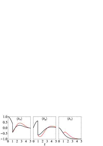
Figure 3: (color online) Plot showing the time evolution of $\langle\hat{\sigma}_{x,y,z}\rangle$. The black curve shows the Markovian dynamics from Eq. (12); the red curve shows the non-Markovian dynamics derived from the total atom-cavity evolution given in Eq. (7).

There are other figure of merits that can also quantify the deviation, e.g., the trace distance between two different atom states Breuer2 , and the entanglement strength between the atom and an introduced ancilla Rivas . In the left panel of Fig. 4, we show the time evolution of the trace distance ${\rm Tr}|\hat{\rho}_{1}(t)-\hat{\rho}_{2}(t)|/2$ with two initial states for the atom given by $\hat{\rho}_{1}(0)=\rm|1\rangle\langle 1|$ and $\hat{\rho}_{2}(0)=\rm|0\rangle\langle 0|$. In the right panel of Fig. 4, we show the time evolution of the concurrence—the ancilla entangled with the atom is another two-level system, and therefore the entanglement strength can be quantified by the concurrence Hill . Initially, the atom and the ancilla are in the maximally-entangled state: $\frac{1}{\sqrt{2}}[|0\rangle|\otimes|0\rangle+|1\rangle|\otimes|1\rangle]$. Other specifications are the same as those for producing Fig. 3. Both the trace distance and the entanglement strength increases after applying the local unitary operation on the atom. Such a revival of the quantum coherence clearly indicates non-Markovianity, just as expected for such a system.

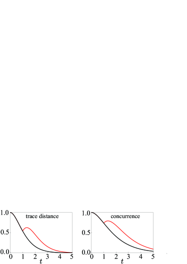
Figure 4: (color online) Plot showing the time evolution of the trace distance (left) and the concurrence (right). The red curve shows the non-Markovian evolution described by Eq. (7) and the black curve is the Markovian evolution from Eq. (10).

Dynamical recovering.—The increase of quantum coherence just shown, when the plant is perturbed with local unitary operations, can be important for quantum-information processing. This allows us to recover information of the plant that is stored in the bath, which we can call “dynamical recovering”. More importantly, by combining local operations with the dynamical decoupling protocols—applying a sequence of control pulses Viloa ; Biercuk ; Lange , we can characterize the plant-bath dynamics even for an unknown bath, which can help us find the optimal strategies for maintaining the quantum coherence.

For illustration, we again use this atom-cavity system. In the left panel of Fig. 5, we show the time evolution of the trace distance for two different dynamical decoupling procedures: (i) the first one is a direct decoupling at $t=1$ by applying a sequence of $\hat{\sigma}_{z}\otimes\hat{I}_{c}$ within short intervals; (ii) the second one is a delayed decoupling (delayed by $\Delta t=0.1$) after the local operation at $t=1$. Their difference in the trace distance tells us how much information of the atom is recovered from the cavity mode, and it varies depending on the delay time $\Delta t$. Interestingly, the maximal difference is achieved when the atom and the cavity mode becomes disentangled, as shown by the right panel of Fig. 5—the concurrence for the atom-cavity entanglement vanishes when the trace distance achieves the local extremum . This is understandable—quantum information of the atom can on longer be recovered from the cavity mode once they are disentangled.

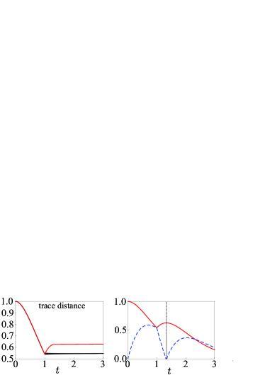
Figure 5: (color online) The left panel shows the time evolution of the trace distance with a direct decoupling (black curve) and a delayed decoupling $\Delta t=0.1$ (red curve) after applying $\hat{\sigma}_{z}\otimes\hat{I}_{c}$ at $t=1$; the right panel shows that the maximal recovering is achieved when the atom and the cavity mode are disentangled [red solid curve is the trace distance (same as the left panel) and the blue dashed curve is the concurrence for the atom-cavity entanglement].

For general plant-bath interactions, starting from any moment during the evolution, there should exist an optimal sequence of local operations on the plant for maximally recovering its information. Operationally, one can define a measure for non-Markovianity based on such dynamical recovering. We introduce the set of plant state pairs with the initial trace distance $D$ that is equal to 1: $\mathcal{A}=\{\{\hat{\rho}_{1}(0),\hat{\rho}_{2}(0)\},\,\forall\,D\{\hat{\rho}_{1}(0),\hat{\rho}_{2}(0)\}=1\}$. Suppose at moment $t$, $D\{\hat{\rho}_{1}(t),\hat{\rho}_{2}(t)\}=\alpha<1$, the measure is:

$${\cal N}_{\alpha}=\max_{\forall\tau,U_{\tau}}\frac{D\{\hat{\Phi}_{U_{\tau}}\hat{\rho}_{1}(t),\hat{\Phi}_{U_{\tau}}\hat{\rho}_{2}(t)\}-\alpha}{1-\alpha},$$ (13)

where $\hat{\Phi}_{U_{\tau}}\hat{\rho}(t)\equiv{\rm Tr}_{b}[\hat{U}_{p}(\tau)\otimes\hat{I}_{b}\,\hat{\rho}_{pb}(t)\hat{U}_{p}^{{\dagger}}(\tau)\otimes\hat{I}_{b}]$ is a sequence of unitary maps for the plant from $t$ to $t+\tau$. Obviously, for Markovian systems, $\mathcal{N}_{\alpha}$ is equal to $0$, and for non-Markovian systems in which the plant can recover its initial states via local operations, the measure is equal to $1$. In general, $\mathcal{N}_{\alpha}$ ranges between $0$ and $1$ depending on how strong the bath memory is, and also the moment $t$ that we start to apply unitary operations.

Discussion.—This criterion can be applied to study the recent experiment by Liu et al. Liu . In their setup, the polarization degree of freedom of photons (the plant) couples to the frequency degrees of freedom (the bath). During the time evolution, these two degrees of freedom become entangled—the polarization undergoes decoherence when tracing over the frequency degrees of freedom. By changing the frequency profile of the bath, i.e., its quantum state, the time evolution of the trace distance for the polarization can either monotonically decrease or oscillate. This was used to demonstrate switching between the Markovian and the non-Markovian regime. Interestingly, if a unitary operation is applied on the polarization by flipping it at a given moment, one will find that the quantum coherence of the polarization will revive at later times even in the so-called Markvoian regime, which indicates that the intrinsic dynamics is non-Markovian as the frequency degrees of freedom contains memory about the polarization. Therefore, this experiment can make a direct test of our new criterion.

Conclusion.—We have presented a new criterion for non-Markovianity in general open quantum systems—the non-Markovianity manifests in terms of non-local change of the dynamical map after applying a local unitary operation on the plant. It allows us to tell whether a time-local positive map is only an artifact of a special initial quantum state of the plant-bath system or not. We have illustrated this criterion with the atom-cavity model. This work, on the one hand, helps clarify some subtleties of non-Markovianity in open quantum systems; on the other hand, it provides a route to probe the non-Markovian bath and to enhance quantum coherence in quantum-information processing.

Acknowledgements.—We thank S.L. Danilishin, F.Ya, Kahlili and other colleagues in the LIGO MQM group for fruitful discussions. This work has been supported by NSF grants PHY-0555406, PHY-0653653, PHY-0601459, PHY-0956189, PHY-1068881, as well as the David and Barbara Groce startup fund at Caltech.

References

- (1) H. P. Breuer and F. Petruccione, The Theory of Open Quantum Systems, Oxford University Press, Oxford (2007).
- (2) M. M. Wolf et al., Phys. Rev. Letter. 101, 150402 (2008).
- (3) H. P. Breuer, E. M. Laine, and J. Piilo, Phys. Rev. Lett. 103, 210401 (2009).
- (4) A. Rivas, S. F. Huelga, and M. B. Plenio, Phys. Rev. Lett. 105, 050403 (2010).
- (5) B. H. Liu et al., Nature Phys. (Advanced online publication) (2011).
- (6) L. Viola, E. Knill, and S. Lloyd, Phys. Rev. Lett. 82, 2417 (1999);
- (7) M. J. Biercuk et al., Nature 458, 996 (2009).
- (8) G. de Lange et al., Science 330, 60 (2010).
- (9) P. Haikka, J. D. Cresser, and S. Maniscalco, Phys. Rev. A 83, 012112 (2011).
- (10) D. Chruściński, A. Kossakowski, and Á Rivas, Phys. Rev. A 83, 052128 (2011).
- (11) V. Gorini, A. Kossakowski, and E. Sudarshan, J. Math. Phys. 17, 821 (1976).
- (12) H. P. Breuer, Phys. Rev. A 70, 012106 (2004).
- (13) D. Chruściński, and A. Kossakowski, Phys. Rev. Lett. 104, 070406 (2010).
- (14) C. W. Gardiner and P. Zoller, Quantum Noise, Springer-Verlag, Berlin, (1991).
- (15) A. Imamoḡlu, Phys. Rev. A 50, 3650 (1994).
- (16) L. Mazzola et al., Phys. Rev. A 80, 012104 (2009).
- (17) H. Yang, H. Miao, and Y. Chen, arXiv:1108.0963 [quant-ph] (2011).
- (18) J. Li, J. Zou, and B. Shao, Phy. Rev. A 81, 062124 (2010).
- (19) S. Hill, and W. K. Wootters, Phys. Rev. Lett. 78, 5022 (1997).