Search for the $Z_{1}(4050)^{+}$ and $Z_{2}(4250)^{+}$ states in $\kern 1.79993pt\overline{\kern-1.79993ptB}{}^{0}\to\chi_{c1}K^{-}\pi^{+}$ and $B^{+}\to\chi_{c1}K^{0}_{\scriptscriptstyle S}\pi^{+}$

Abstract

We search for the $Z_{1}(4050)^{+}$ and $Z_{2}(4250)^{+}$ states, reported by the Belle Collaboration, decaying to $\chi_{c1}\pi^{+}$ in the decays $\kern 1.79993pt\overline{\kern-1.79993ptB}{}^{0}\to\chi_{c1}K^{-}\pi^{+}$ and $B^{+}\to\chi_{c1}K^{0}_{\scriptscriptstyle S}\pi^{+}$ where $\chi_{c1}\to{J\mskip-3.0mu/\mskip-2.0mu\psi\mskip 2.0mu}\gamma$. The data were collected with the BABAR detector at the SLAC PEP-II asymmetric-energy $e^{+}e^{-}$ collider operating at center-of-mass energy 10.58 $\mathrm{\,Ge\kern-1.00006ptV\!}$, and correspond to an integrated luminosity of 429 fb^-1. In this analysis, we model the background-subtracted, efficiency-corrected $\chi_{c1}\pi^{+}$ mass distribution using the $K\pi$ mass distribution and the corresponding normalized $K\pi$ Legendre polynomial moments, and then test the need for the inclusion of resonant structures in the description of the $\chi_{c1}\pi^{+}$ mass distribution. No evidence is found for the $Z_{1}(4050)^{+}$ and $Z_{2}(4250)^{+}$ resonances, and 90% confidence level upper limits on the branching fractions are reported for the corresponding $B$-meson decay modes.

I Introduction

The Belle Collaboration has reported the observation of two resonance-like structures in the study of $\kern 1.79993pt\overline{\kern-1.79993ptB}{}^{0}\to\chi_{c1}K^{-}\pi^{+}$ belle3 . These are labeled as $Z_{1}(4050)^{+}$ and $Z_{2}(4250)^{+}$, both decaying to $\chi_{c1}\pi^{+}$ PDG . The Belle Collaboration also reported the observation of a resonance-like structure, $Z(4430)^{+}\to\psi{(2S)}\pi^{+}$ in the analysis of $B\to\psi{(2S)}K\pi$ belle1 ; belle2 . These claims have generated a great deal of interest theory . Such states must have a minimum quark content $c\bar{c}\bar{d}u$, and thus would represent an unequivocal manifestation of four-quark meson states.

The BABAR Collaboration did not see the $Z(4430)^{+}$ in an analysis of the decay $B\to\psi{(2S)}K\pi$ babarz . Points of discussion are:

• The method of making slices of a three-body $B$ decay Dalitz plot can produce peaks which may be due to interference effects, not resonances.

• The angular structure of the $B\to\psi{(2S)}K\pi$ decay is rather complex and cannot be described adequately by only the two variables used in a simple Dalitz plot analysis.

In the BABAR analysis babarz , the $B\to{J\mskip-3.0mu/\mskip-2.0mu\psi\mskip 2.0mu}K\pi$ decay does not show evidence for resonances neither in ${J\mskip-3.0mu/\mskip-2.0mu\psi\mskip 2.0mu}\pi$ nor in ${J\mskip-3.0mu/\mskip-2.0mu\psi\mskip 2.0mu}K$ systems. All resonance activity seems confined to the $K\pi$ system. It is also observed that the angular distributions, expressed in terms of the $K\pi$ Legendre polynomial moments, show strong similarities between $B\to\psi{(2S)}K\pi$ and $B\to{J\mskip-3.0mu/\mskip-2.0mu\psi\mskip 2.0mu}K\pi$ decays. Therefore, the angular information provided by the $B\to{J\mskip-3.0mu/\mskip-2.0mu\psi\mskip 2.0mu}K\pi$ decay can be used to describe the $B\to\psi{(2S)}K\pi$ decay. It is also observed that a localized structure in the $\psi{(2S)}\pi$ mass spectrum would yield high angular momentum Legendre polynomial moments in the $K\pi$ system. Therefore, a good description of the $\psi{(2S)}\pi$ data using only $K\pi$ moments up to $L=5$ also suggests the absence of narrow resonant structure in the $\psi{(2S)}\pi$ system.

In this paper, we examine $B\to\chi_{c1}K\pi$ decays following an analysis procedure similar to that used in Ref. babarz . In contrast to the analysis of Ref belle3 , we model the background-subtracted, efficiency-corrected $\chi_{c1}\pi^{+}$ mass distribution using the $K\pi$ mass distribution and the corresponding normalized $K\pi$ Legendre polynomial moments, and then test the need for the inclusion of resonant structures in the description of the $\chi_{c1}\pi^{+}$ mass distribution.

This paper is organized as follows. A short description of the BABAR experiment is given in Sec. II, and the data selection is described in Sec. III. Section IV shows the data, while Sec. V and Sec. VI are devoted to the calculation of the efficiency and the extraction of branching fraction values, respectively. In Sec. VII we describe the fits to the $K\pi$ mass spectra, and in Sec. VIII we show the Legendre polynomial moments. In Sec. IX we report the description of the $\chi_{c1}\pi^{+}$ mass spectra, while Sec. X is devoted to the calculation of limits on the production of the $Z_{1}(4050)^{+}$ and $Z_{2}(4250)^{+}$ resonances. We summarize our results in Sec. XI.

II The BABAR experiment

This analysis is based on a data sample of 429 $\mbox{\,fb}^{-1}$ recorded at the $\Upsilon{(4S)}$ resonance by the BABAR detector at the PEP-II asymmetric-energy $e^{+}e^{-}$ storage rings. The BABAR detector is described in detail elsewhere babar . Charged particles are detected and their momenta measured with a combination of a cylindrical drift chamber (DCH) and a silicon vertex tracker (SVT), both operating within the 1.5 T magnetic field of a superconducting solenoid. Information from a ring-imaging Cherenkov detector is combined with specific ionization measurements from the SVT and DCH to identify charged kaon and pion candidates. Photon energy and position are measured with a CsI(Tl) electromagnetic calorimeter (EMC), which is also used to identify electrons. The return yoke of the superconducting coil is instrumented with resistive plate chambers for the identification of muons. For the later part of the experiment the barrel-region chambers were replaced by limited streamer tubes lst .

III Data Selection

We reconstruct events in the decay modes conj :

$$\kern 1.79993pt\overline{\kern-1.79993ptB}{}^{0}\to\chi_{c1}K^{-}\pi^{+}\,,$$ (1)

$$B^{+}\to\chi_{c1}K^{0}_{\scriptscriptstyle S}\pi^{+}\,,$$ (2)

where $\chi_{c1}\to{J\mskip-3.0mu/\mskip-2.0mu\psi\mskip 2.0mu}\gamma$, and ${J\mskip-3.0mu/\mskip-2.0mu\psi\mskip 2.0mu}\to\mu^{+}\mu^{-}$ or ${J\mskip-3.0mu/\mskip-2.0mu\psi\mskip 2.0mu}\to e^{+}e^{-}$.

For each candidate, we first reconstruct the ${J\mskip-3.0mu/\mskip-2.0mu\psi\mskip 2.0mu}$ by geometrically constraining an identified $e^{+}e^{-}$ or $\mu^{+}\mu^{-}$ pair of tracks to a common vertex point and requiring a $\chi^{2}$ fit probability greater than 0.1%. For ${J\mskip-3.0mu/\mskip-2.0mu\psi\mskip 2.0mu}\to e^{+}e^{-}$ we introduce bremsstrahlung energy-loss recovery. If an electron-associated photon cluster is found in the EMC, its three-momentum vector is incorporated into the calculation of $m(e^{+}e^{-})$ brem . The fit to the ${J\mskip-3.0mu/\mskip-2.0mu\psi\mskip 2.0mu}$ candidates includes the constraint to the nominal ${J\mskip-3.0mu/\mskip-2.0mu\psi\mskip 2.0mu}$ mass value PDG .

A $K^{0}_{\scriptscriptstyle S}$ candidate is formed by geometrically constraining a pair of oppositely charged tracks to a common vertex ($\chi^{2}$ fit probability greater than 0.1%). For the two tracks the pion mass is assumed without particle-identification requirements. The $K^{0}_{\scriptscriptstyle S}$ fit includes the constraint to the nominal mass value.

The ${J\mskip-3.0mu/\mskip-2.0mu\psi\mskip 2.0mu}$, $K^{\pm}$, and $\pi^{\pm}$ candidates forming a $B$ meson decay candidate are geometrically constrained to a common vertex and a $\chi^{2}$ fit probability greater than 0.1% is required. Particle identification is applied to both $K$ and $\pi$ candidates. The $K^{0}_{\scriptscriptstyle S}$ flight length with respect to the $B^{+}$ vertex must be greater than 0.2 cm.

A study of the scatter diagram $E_{\gamma}$ vs. $m({J\mskip-3.0mu/\mskip-2.0mu\psi\mskip 2.0mu}\gamma)$ (not shown) reveals that no $\chi_{c1}$ signal is kinematically possible for $E_{\gamma}<190$ MeV. Therefore, we consider only photons with a laboratory energy above this value. We select the $\chi_{c1}$ signal within $\pm 2\ \sigma_{\chi_{c1}}$ of the $\chi_{c1}$ mass, where $\sigma_{\chi_{c1}}$ and the $\chi_{c1}$ mass are obtained from fits to the ${J\mskip-3.0mu/\mskip-2.0mu\psi\mskip 2.0mu}\gamma$ mass spectra using a Gaussian function for the signal and a $2^{\rm nd}$-order polynomial for the background, separated by $B$ and ${J\mskip-3.0mu/\mskip-2.0mu\psi\mskip 2.0mu}$ decay mode. The values of $\sigma_{\chi_{c1}}$ range from 14.6 ${\mathrm{\,Me\kern-1.00006ptV\!/}c^{2}}$ to 17.6 ${\mathrm{\,Me\kern-1.00006ptV\!/}c^{2}}$.

We further define $B$ meson decay candidates using the energy difference $\mbox{$\Delta E$}\equiv E^{\ast}_{B}-\sqrt{s}/2$ in the center-of-mass (c.m.) frame and the beam-energy-substituted mass defined as $\mbox{$m_{\rm ES}$}\equiv\sqrt{((s/2+\vec{p}_{i}\cdot\vec{p}_{B})/E_{i})^{2}-\vec{p}_{B}^{\,2}}$, where ($E_{i},\vec{p}_{i}$) is the initial state $e^{+}e^{-}$ four-momentum vector in the laboratory frame and $\sqrt{s}$ is the c.m. energy. In the above expressions $E^{\ast}_{B}$ is the $B$ meson candidate energy in the c.m. frame, and $\vec{p}_{B}$ is its laboratory frame momentum. The $B$ decay signal events are selected within $\pm 2.0\ \sigma_{\mbox{$m_{\rm ES}$}}$ of the fitted central value, where the $\sigma_{\mbox{$m_{\rm ES}$}}$ values are listed in Table 1 and are determined by fits of a Gaussian function plus an ARGUS function argus to the data.

The resulting $\Delta E$ distributions have been fitted with a linear background function and a signal Gaussian function whose width values ($\sigma_{\mbox{$\Delta E$}}$) are also listed in Table 1. Further background rejection is performed by selecting events within $\pm 2.0\ \sigma_{\mbox{$\Delta E$}}$ of zero. Table 1 also gives the values of event yield and purity, where the Purity is defined as Signal/(Signal+Background). The $\Delta E$ distributions shown in Fig. 1 have been summed over the ${J\mskip-3.0mu/\mskip-2.0mu\psi\mskip 2.0mu}\to\mu^{+}\mu^{-}$ and ${J\mskip-3.0mu/\mskip-2.0mu\psi\mskip 2.0mu}\to e^{+}e^{-}$ decay modes. Clear signals of the $B$ decay modes (1) and (2) can be seen. We obtain 1863 candidates for $\kern 1.79993pt\overline{\kern-1.79993ptB}{}^{0}\to\chi_{c1}K^{-}\pi^{+}$ decays with 78% purity, and 628 $B^{+}\to\chi_{c1}K^{0}_{\scriptscriptstyle S}\pi^{+}$ events with 79% purity. A study of the $\Delta E$ and ${J\mskip-3.0mu/\mskip-2.0mu\psi\mskip 2.0mu}\gamma$ spectra in the sideband regions does not show any $B$ or $\chi_{c1}$ signal respectively. We conclude that the observed background is consistent with being entirely of combinatorial origin.

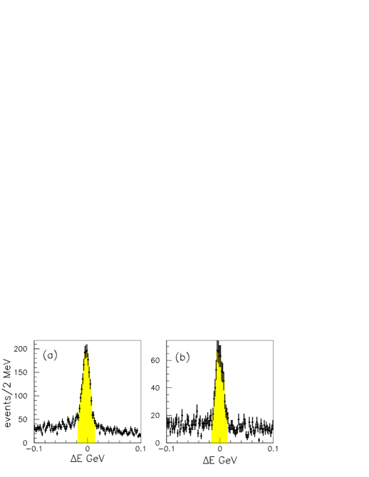
Figure 1: Distributions of $\Delta E$ for (a) $\kern 1.79993pt\overline{\kern-1.79993ptB}{}^{0}\to\chi_{c1}K^{-}\pi^{+}$ and (b) $B^{+}\to\chi_{c1}K^{0}_{\scriptscriptstyle S}\pi^{+}$ summed over the ${J\mskip-3.0mu/\mskip-2.0mu\psi\mskip 2.0mu}$ decay modes; the $\chi_{c1}$ and $m_{\rm ES}$ selection criteria have been applied. The shaded areas indicate the signal regions.

The resulting ${J\mskip-3.0mu/\mskip-2.0mu\psi\mskip 2.0mu}\gamma$ invariant mass distributions for channels (1) and (2) are shown in Fig. 2.

In order to estimate the background contribution in the signal region, we define $\Delta E$ sideband regions in the intervals $(7-9)\ \sigma_{\mbox{$\Delta E$}}$ on both sides of zero. We obtain a “background-subtracted” distribution of events by subtracting the corresponding distribution for $\Delta E$ sideband events from that of events in the signal region.

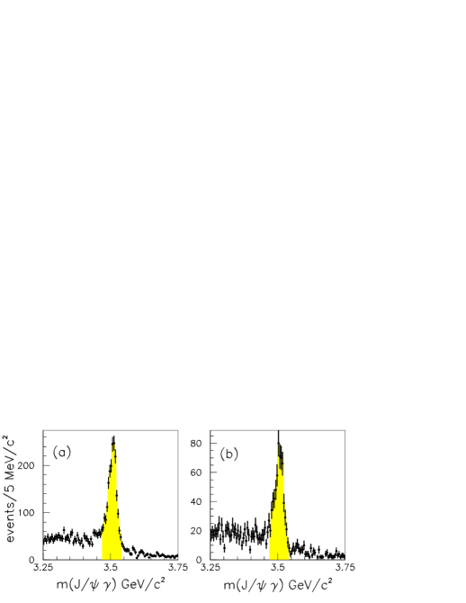
Figure 2: The ${J\mskip-3.0mu/\mskip-2.0mu\psi\mskip 2.0mu}\gamma$ mass distribution for (a) $\kern 1.79993pt\overline{\kern-1.79993ptB}{}^{0}\to\chi_{c1}K^{-}\pi^{+}$ and (b) $B^{+}\to\chi_{c1}K^{0}_{\scriptscriptstyle S}\pi^{+}$ candidates, summed over the ${J\mskip-3.0mu/\mskip-2.0mu\psi\mskip 2.0mu}$ decay modes. The $m_{\rm ES}$ and $\Delta E$ selection criteria have been applied. The shaded areas indicate the signal regions.

Table 1: Resolution parameter values from fits to the $\Delta E$ and $m_{\rm ES}$ distributions.

Channel	$\sigma_{\mbox{$\Delta E$}}\ (\mathrm{\,Me\kern-1.00006ptV\!})$	$\sigma_{\mbox{$m_{\rm ES}$}}\ ({\mathrm{\,Me\kern-1.00006ptV\!/}c^{2}})$	events	Purity %
$\kern 1.79993pt\overline{\kern-1.79993ptB}{}^{0}\to\chi_{c1}K^{-}\pi^{+}$ ($\mu^{+}\mu^{-}$)	6.96 $\pm$ 0.34	2.60 $\pm$ 0.10	980	79.3 $\pm$ 1.3
$\kern 1.79993pt\overline{\kern-1.79993ptB}{}^{0}\to\chi_{c1}K^{-}\pi^{+}$ ($e^{+}e^{-}$)	7.81 $\pm$ 0.43	2.77 $\pm$ 0.12	883	77.1 $\pm$ 1.4
$B^{+}\to\chi_{c1}K^{0}_{\scriptscriptstyle S}\pi^{+}$ ($\mu^{+}\mu^{-}$)	6.65 $\pm$ 0.55	2.65 $\pm$ 0.27	299	81.7 $\pm$ 2.2
$B^{+}\to\chi_{c1}K^{0}_{\scriptscriptstyle S}\pi^{+}$ ($e^{+}e^{-}$)	7.52 $\pm$ 0.70	2.65 $\pm$ 0.18	329	77.5 $\pm$ 2.3

IV Dalitz plots

The Dalitz plots for $\kern 1.79993pt\overline{\kern-1.79993ptB}{}^{0}\to\chi_{c1}K^{-}\pi^{+}$ events in the signal and sideband regions are shown in Fig. 3. The shaded area defines the Dalitz plot boundary; it is obtained from a simple phase space Monte Carlo (MC) simulation genbod of $B$ decays, smeared by the experimental resolution. For the sidebands, events can lie outside the boundary.

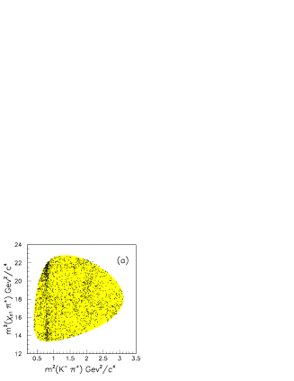
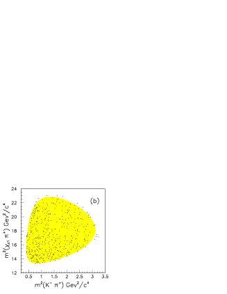
Figure 3: Dalitz plot for $\kern 1.79993pt\overline{\kern-1.79993ptB}{}^{0}\to\chi_{c1}K^{-}\pi^{+}$ in (a) the signal region and (b) the $\Delta E$ sidebands. The shaded area defines the Dalitz plot boundary.

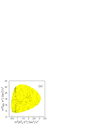
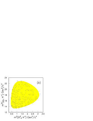
Figure 4: Dalitz plot for $B^{+}\to\chi_{c1}K^{0}_{\scriptscriptstyle S}\pi^{+}$ in (a) the signal region and (b) the $\Delta E$ sidebands. The shaded area defines the Dalitz plot boundary.

We observe a vertical band due to the presence of the $\overline{K^{*}}(892)^{0}$ resonance and a weaker band due to the $\overline{K^{*}_{2}}(1430)^{0}$ resonance. We do not observe significant accumulation of events in any horizontal band.

The Dalitz plots for $B^{+}\to\chi_{c1}K^{0}_{\scriptscriptstyle S}\pi^{+}$ candidates in the signal and sideband regions are shown in Fig. 4 and show features similar to those in Fig. 3.

V Efficiency

To compute the efficiency, signal MC events (full-MC) for the different channels have been generated using a detailed detector simulation where $B$ mesons decay uniformly in phase space. They are reconstructed and analyzed in the same way as real events. We express the efficiency as a function of $m(K\pi)$ and $\cos\theta$, the normalized dot-product between the $\chi_{c1}$ momentum and that of the kaon momentum, both in the $K\pi$ rest frame. To smooth statistical fluctuations, this efficiency is then parametrized as follows.

We first fit the efficiency as a function of $\cos\theta$ in separate 50 ${\mathrm{\,Me\kern-1.00006ptV\!/}c^{2}}$ intervals of $m(K\pi)$, in terms of Legendre polynomials up to $L=12$:

$$\epsilon(\cos\theta)=\sum_{L=0}^{12}a_{L}(m)Y^{0}_{L}(\cos\theta).$$ (3)

For each value of $L$, we fit the $a_{L}(m)$ as a function of $m(K\pi)$ using a $6^{\rm th}$-order polynomial in $m(K\pi)$. The resulting fitted efficiency for $\kern 1.79993pt\overline{\kern-1.79993ptB}{}^{0}$ decay is shown in Fig. 5(a). We observe a significant decrease in efficiency for $\cos\theta\sim+1$ and $0.72<m(K^{-}\pi^{+})<0.92$ ${\mathrm{\,Ge\kern-1.00006ptV\!/}c^{2}}$, and for $\cos\theta\sim-1$ and $0.97<m(K^{-}\pi^{+})<1.27$ ${\mathrm{\,Ge\kern-1.00006ptV\!/}c^{2}}$. The former is due to the failure to reconstruct pions with low momentum in the laboratory frame and the latter to a similar failure for kaons. A similar effect is observed in Fig. 5(b) for the the $B^{+}$ decay mode.

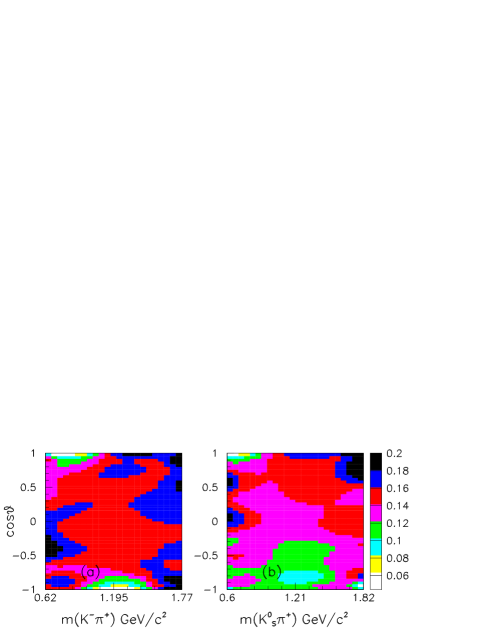
Figure 5: Fitted efficiency on the $\cos\theta\ vs.\ m(K\pi)$ plane for (a) $\kern 1.79993pt\overline{\kern-1.79993ptB}{}^{0}\to\chi_{c1}K^{-}\pi^{+}$ and (b) $B^{+}\to\chi_{c1}K^{0}_{\scriptscriptstyle S}\pi^{+}$ summed over the ${J\mskip-3.0mu/\mskip-2.0mu\psi\mskip 2.0mu}$ decay modes.

In Fig. 6 we plot the efficiency projection as a function of $m(\chi_{c1}\pi^{+})$ for channels (1) and (2), summed over the ${J\mskip-3.0mu/\mskip-2.0mu\psi\mskip 2.0mu}$ decay modes.

Figure 6: Efficiency as a function of $m(\chi_{c1}\pi^{+})$ for (a) $\kern 1.79993pt\overline{\kern-1.79993ptB}{}^{0}\to\chi_{c1}K^{-}\pi^{+}$ and (b) $B^{+}\to\chi_{c1}K^{0}_{\scriptscriptstyle S}\pi^{+}$ summed over the ${J\mskip-3.0mu/\mskip-2.0mu\psi\mskip 2.0mu}$ decay modes.

We observe a loss in efficiency at the edges of the $\chi_{c1}\pi^{+}$ mass range. However these losses do not affect the regions of the reported $Z$ resonances. Using these fitted functions we obtain efficiency-corrected distributions by weighting each event by the inverse of the efficiency at its $(m(K\pi),\cos\theta)$ location.

VI Branching Fractions

We measure the branching fractions for $\kern 1.79993pt\overline{\kern-1.79993ptB}{}^{0}\to\chi_{c1}K^{-}\pi^{+}$ and $B^{+}\to\chi_{c1}K^{0}_{\scriptscriptstyle S}\pi^{+}$ relative to $B^{0}\to J/\psi K^{+}\pi^{-}$ and $B^{+}\to J/\psi K^{0}_{\scriptscriptstyle S}\pi^{+}$, respectively. In this way several systematic uncertainties, (namely uncertainties on the number of $B\bar{B}$ mesons, particle identification, tracking efficiency, data-MC differences, secondary branching fractions) cancel.

To obtain the yields, for each $B$ decay mode we perform new fits to the $\Delta E$ distributions using the full-MC lineshape for the signal and a linear background. The background-subtracted data are then integrated between $\pm 2.0\ \sigma_{\mbox{$\Delta E$}}$. The correction for efficiency is obtained as described in Sec. V. A similar procedure is applied to the $\kern 1.79993pt\overline{\kern-1.79993ptB}{}^{0}\to J/\psi K^{-}\pi^{+}$ and $B^{+}\to J/\psi K^{0}_{\scriptscriptstyle S}\pi^{+}$ data.

The branching fraction for $\chi_{c1}\to J/\psi\gamma$ from Ref. PDG is $0.344\pm 0.015$. Using this value, we obtain the following branching fraction ratios:

$$\frac{{\cal B}(\kern 1.79993pt\overline{\kern-1.79993ptB}{}^{0}\to\chi_{c1}K^{-}\pi^{+})}{{\cal B}(\kern 1.79993pt\overline{\kern-1.79993ptB}{}^{0}\to J/\psi K^{-}\pi^{+})}=0.474\pm 0.013\pm 0.026,$$ (4)

and

$$\frac{{\cal B}(B^{+}\to\chi_{c1}K^{0}\pi^{+})}{{\cal B}(B^{+}\to J/\psi K^{0}\pi^{+})}=0.501\pm 0.024\pm 0.028.$$ (5)

Systematic uncertainties are summarized in Table 2 and have been evaluated as follows:

1. We obtain the uncertainty on the background subtraction by modifying the model used to fit the $\Delta E$ distributions. The signal was alternatively described by the sum of two Gaussian functions and the background was parametrized by a $2^{\rm nd}$-order polynomial.

2. We compute the uncertainty on the efficiency by making use of the binned efficiency on the $(m(K\pi),\cos\theta)$ plane. In each cell we randomize the generated and reconstructed yields according to Poisson distributions. Deviations from the fitted efficiencies give the uncertainty on this quantity.

3. We vary the bin size for the binned efficiency calculation.

4. We include a systematic error due to the uncertainty on the $\chi_{c1}\to{J\mskip-3.0mu/\mskip-2.0mu\psi\mskip 2.0mu}\gamma$ branching fraction PDG .

5. We assign a 1.8 % uncertainty to the $\gamma$ reconstruction efficiency.

6. We modify the $\Delta E$ and $m_{\rm ES}$ selection criteria and assign systematic uncertainties based on the variation of the extracted branching fractions.

We note that the systematic uncertainties are dominated by the uncertainty on the $\chi_{c1}\to{J\mskip-3.0mu/\mskip-2.0mu\psi\mskip 2.0mu}\gamma$ branching fraction.

Table 2: Systematic uncertainties (%) for the $B\to\chi_{c1}K\pi$ relative branching fraction measurements.

Contribution	$\kern 1.61993pt\overline{\kern-1.61993ptB}{}^{0}\to\chi_{c1}K^{-}\pi^{+}$	$B^{+}\to\chi_{c1}K^{0}_{\scriptscriptstyle S}\pi^{+}$
1. Background subtraction	1.6	1.0
2. Efficiency	1.5	1.6
3. Efficiency binning	1.1	1.9
4. $\chi_{c1}$ branching fraction	4.4	4.4
5. $\gamma$ reconstruction	1.8	1.8
6. $\Delta E$ and $m_{\rm ES}$ selections	1.0	1.0
Total (%)	5.4	5.5

The branching fractions measured in Ref. babarz are:

$${\cal B}(\kern 1.79993pt\overline{\kern-1.79993ptB}{}^{0}\to J/\psi K^{-}\pi^{+})=(1.079\pm 0.011)\times 10^{-3},$$ (6)

$${\cal B}(B^{+}\to J/\psi K^{0}\pi^{+})=(1.101\pm 0.021)\times 10^{-3},$$ (7)

where the latter value has been corrected for $K^{0}_{\scriptscriptstyle L}$ and $K^{0}_{\scriptscriptstyle S}\to\pi^{0}\pi^{0}$ decays PDG .

Multiplying the ratio in Eq. (4) by the $\kern 1.79993pt\overline{\kern-1.79993ptB}{}^{0}\to J/\psi K^{-}\pi^{+}$ branching fraction in Eq. (6) we obtain

$${\cal B}(\kern 1.79993pt\overline{\kern-1.79993ptB}{}^{0}\to\chi_{c1}K^{-}\pi^{+})=(5.11\pm 0.14\pm 0.28)\times 10^{-4}.$$ (8)

This may be compared to the Belle measurement belle3 : ${\cal B}(\kern 1.79993pt\overline{\kern-1.79993ptB}{}^{0}\to\chi_{c1}K^{-}\pi^{+})=(3.83\pm 0.10\pm 0.39)\times 10^{-4}$.

Multiplying the ratio in Eq. (5) by the $B^{+}\to J/\psi K^{0}\pi^{+}$ branching fraction in Eq. (7) we obtain

$${\cal B}(B^{+}\to\chi_{c1}K^{0}\pi^{+})=(5.52\pm 0.26\pm 0.31)\times 10^{-4},$$ (9)

so that, after all corrections, the branching fractions corresponding to decay modes (1) and (2) are the same within uncertainties.

VII Fits to the $K\pi$ mass spectra

We perform binned-$\chi^{2}$ fits to the background-subtracted and efficiency-corrected $K\pi$ mass spectra in terms of $S$, $P$, and $D$ wave amplitudes. The fitting function is expressed as:

$$\frac{dN}{dm}=N\times$$

$$\left[f_{S}\frac{G_{S}(m)}{\int G_{S}(m)dm}+f_{P}\frac{G_{P}(m)}{\int G_{P}(m)dm}+f_{D}\frac{G_{D}(m)}{\int G_{D}(m)dm}\right]\ ,$$

where $m=m(K\pi)$, the integrals are over the full $m(K\pi)$ range, and the fractions $f$ are such that

$$f_{S}+f_{P}+f_{D}=1\,.$$ (11)

The $P$- and $D$-wave intensities, $G_{P}(m)$ and $G_{D}(m)$, are expressed in terms of the squared moduli of relativistic Breit-Wigner functions with parameters fixed to the PDG values for $K^{*}(892)$ and $K^{*}_{2}(1430)$ respectively PDG . For the S-wave contribution $G_{S}(m)$ we make use of the LASS lass parametrization described by Eqs. (11)-(16) of Ref. babarz .

The above model gives a good description of the data for the decays $B\to{J\mskip-3.0mu/\mskip-2.0mu\psi\mskip 2.0mu}K\pi$ babarz . However, for $B\to\chi_{c1}K\pi$ the above resonances do not describe the high mass region of the $K\pi$ mass spectra well. A better fit is obtained by including an additional incoherent spin-1 $K^{*}(1680)$ PDG resonance contribution. The fit results are shown by the solid curves in Fig. 7, and the resulting intensity contributions are summarized in Table 3. In Figures 7(a) and  7(b) the contributions due to the $K^{*}(1680)$ amplitude are shown by the dashed curves. The $\chi_{c1}K\pi$ decay modes differ from the corresponding ${J\mskip-3.0mu/\mskip-2.0mu\psi\mskip 2.0mu}K\pi$ and $\psi(2S)K\pi$ decay modes in that the $S$-wave fraction is much larger in the former than in the latter. This was observed for the $K^{*}(892)$ region in a previous BABAR analysis babar2 .

Table 3: $S$, $P$, $D$ wave fractions (in %), and $\chi^{2}/{\rm NDF}$ (NDF = Number of Degrees of Freedom) from the fits to the $K\pi$ mass spectra in $\kern 1.79993pt\overline{\kern-1.79993ptB}{}^{0}\to\chi_{c1}K^{-}\pi^{+}$ and $B^{+}\to\chi_{c1}K^{0}_{\scriptscriptstyle S}\pi^{+}$. The second $P$-wave entry in the two $\chi_{c1}$ channels corresponds to the fraction of $K^{*}(1680)$.

Channel	$S$-wave	$P$-wave	$D$-wave	$\chi^{2}/{\rm NDF}$
$\kern 1.79993pt\overline{\kern-1.79993ptB}{}^{0}\to\chi_{c1}K^{-}\pi^{+}$	40.4 $\pm$ 2.2	37.9 $\pm$ 1.3	11.4 $\pm$ 2.0	58/54
		10.3 $\pm$ 1.5
$B^{+}\to\chi_{c1}K^{0}_{\scriptscriptstyle S}\pi^{+}$	42.4 $\pm$ 3.5	37.1 $\pm$ 3.2	10.1 $\pm$ 3.1	55/54
		10.4 $\pm$ 2.5

Figure 7: Fits to the background-subtracted and efficiency-corrected $K\pi$ mass spectra for (a) $\kern 1.79993pt\overline{\kern-1.79993ptB}{}^{0}\to\chi_{c1}K^{-}\pi^{+}$ and (b) $B^{+}\to\chi_{c1}K^{0}_{\scriptscriptstyle S}\pi^{+}$. The $K^{*}(1680)$ contribution is shown in each figure by the dashed curve.

VIII The $K\pi$ Legendre polynomial moments

We compute the efficiency-corrected Legendre polynomial moments $<Y^{0}_{L}>$ in each $K\pi$ mass interval by correcting for efficiency, as explained in Sec. V, and then weighting each event by the $Y^{0}_{L}(\cos\theta)$ functions. A similar procedure is performed for the $\Delta E$ sideband events, for which the distributions are subtracted from those in the signal region. We observe consistency between the $\kern 1.79993pt\overline{\kern-1.79993ptB}{}^{0}$ and $B^{+}$ data. Therefore, in the following we combine the $\kern 1.79993pt\overline{\kern-1.79993ptB}{}^{0}$ and $B^{+}$ distributions.

This yields the background-subtracted and efficiency-corrected Legendre polynomial moments $<Y^{0}_{L}>$. They are shown for $L=1,...,6$ in Fig. 8. We notice that the $<Y^{0}_{6}>$ moment is consistent with zero, as are higher moments (not shown).

Figure 8: Legendre polynomial moments $<Y^{0}_{L}>$ for $L=1,...,6$ as functions of $K\pi$ mass for $B\to\chi_{c1}K\pi$ after background-subtraction and efficiency-correction.

These moments can be expressed in terms of $S$-, $P$- and $D$-wave $K\pi$ amplitudes Stephane . The $P$- and $D$-waves can be present in three helicity states and, after integration over the decay angles of the $\chi_{c1}$, the relationship between the moments and the amplitudes is given by Eqs. (26)-(30) of Ref. babarz . We notice that, ignoring the presence of resonances in the exotic charmonium channel, the equations involve seven amplitude magnitudes and six relative phase values, and so they cannot be solved in each $m(K\pi)$ interval. For this reason, it is not possible to extract the amplitude moduli and relative phase values from Dalitz plot analyses of the $\psi K\pi$ or $\chi_{c1}K\pi$ final states.

In Fig. 8 we observe the presence of the spin-1 $K^{*}(890)$ in the $<Y_{2}^{0}>$ moment and $S$-$P$ interference in the $<Y_{1}^{0}>$ moment. We also observe evidence for the spin-2 $K^{*}_{2}(1430)$ resonance in the $<Y_{4}^{0}>$ moment. There are some similarities between the moments of Fig. 8 and those from $B\to{J\mskip-3.0mu/\mskip-2.0mu\psi\mskip 2.0mu}K\pi$ decays in Ref. babarz . However we also observe a significant structure around 1.7 ${\mathrm{\,Ge\kern-1.00006ptV\!/}c^{2}}$ in $<Y_{1}^{0}>$ which is absent in the $B\to{J\mskip-3.0mu/\mskip-2.0mu\psi\mskip 2.0mu}K\pi$ decays. We attribute this to the presence of the $K^{*}_{1}(1680)$ resonance produced in $B\to\chi_{c1}K\pi$ but absent in $B\to{J\mskip-3.0mu/\mskip-2.0mu\psi\mskip 2.0mu}K\pi$. The presence of scalar $Z$ resonances should show up especially in high $<Y_{L}^{0}>$ moments.

From the $<Y_{L}^{0}>$ we obtain the normalized moments

$$<Y_{L}^{N}>=\frac{<Y_{L}^{0}>}{n},$$ (12)

where $n$ is the number of events in the given $m(K\pi)$ mass interval.

IX Monte Carlo Simulations

We model $B\to\chi_{c1}K\pi$ using the resonant structure obtained from the analysis of the $K\pi$ mass spectra and $K\pi$ Legendre polynomial moments. For this purpose we generate a large number of MC events according to the following procedure.

• $B\to\chi_{c1}K\pi$ events are generated uniformly in phase space genbod . The $B$ mass is generated as a Gaussian lineshape with parameters obtained from a fit to the data.

• We weight each event by a factor $w_{m(K\pi)}$ derived from the resonant structure in the $K\pi$ system described in Sec. VII (Eq. (10)), and displayed in Table 3.

• We incorporate the measured $K\pi$ angular structure by giving weight $w_{L}$ to each event according to the expression:

  $$w_{L}=\sum_{i=0}^{L_{\rm max}}<Y_{i}^{N}>Y^{0}_{i}(\cos\theta).$$ (13)

  The moments correspond to the combined data from the decay modes of Eqs. (1) and (2). The $<Y_{i}^{N}>$ are evaluated for the $m(K\pi)$ value by linear interpolation between consecutive $m(K\pi)$ mass intervals.

• The total weight is thus:

  $$w=w_{m(K\pi)}\cdot w_{L}$$ (14)

The generated distributions, weighted by the total weight $w$, are then normalized to the number of data events obtained after background-subtraction and efficiency-correction.

We first test the method using as control sample the combined data from $\kern 1.79993pt\overline{\kern-1.79993ptB}{}^{0}\to{J\mskip-3.0mu/\mskip-2.0mu\psi\mskip 2.0mu}K^{-}\pi^{+}$ and $B^{+}\to{J\mskip-3.0mu/\mskip-2.0mu\psi\mskip 2.0mu}K^{0}_{\scriptscriptstyle S}\pi^{+}$, where no resonant structure is observed in the ${J\mskip-3.0mu/\mskip-2.0mu\psi\mskip 2.0mu}\pi$ mass distributions babarz . In this case we generate $B\to{J\mskip-3.0mu/\mskip-2.0mu\psi\mskip 2.0mu}K\pi$ events and use the $K\pi$ resonant structure and Legendre polynomial information from the same channels. We compare the MC simulation to the ${J\mskip-3.0mu/\mskip-2.0mu\psi\mskip 2.0mu}\pi^{+}$ mass projection from data in Fig. 9. We obtain $\chi^{2}/{\rm NDF}=223,162,180/152$ for $L_{\rm max}=4,5,6$ respectively. We conclude that $L_{\rm max}=5$ gives the best description of the data.

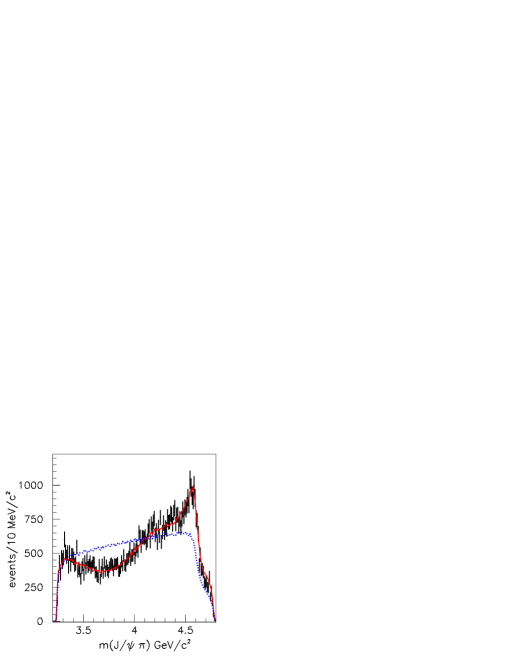
Figure 9: Background-subtracted and efficiency-corrected ${J\mskip-3.0mu/\mskip-2.0mu\psi\mskip 2.0mu}\pi$ mass distribution for the $B\to{J\mskip-3.0mu/\mskip-2.0mu\psi\mskip 2.0mu}K\pi$ control sample with the superimposed curves resulting from the MC simulation described in the text. The solid curve is obtained using the total weight $w$ obtained with $L_{\rm max}=5$, the dotted curve by omitting the angular-dependence factor $w_{L}$.

Table 4: The value of $\chi^{2}/{\rm NDF}$ for different MC-data comparisons; “$Y^{N}_{L}$” indicates the channel used to obtain the normalized moments. The “mixed” algorithm is explained in the text. The definition of window is given in Sec. X.

Channel	$Y^{N}_{L}$	$L_{\rm max}$	$\chi^{2}/{\rm NDF}$
$B\to J/\psi K\pi$	$B\to J/\psi K\pi$	5	162/152
$B\to\chi_{c1}K\pi$	$B\to\chi_{c1}K\pi$	5	46/58
$B\to\chi_{c1}K\pi$	$B\to\chi_{c1}K\pi$	“mixed”	63/58
$B\to\chi_{c1}K\pi$ window	$B\to\chi_{c1}K\pi$	5	45/47
$B\to\chi_{c1}K\pi$ window	$B\to\chi_{c1}K\pi$	“mixed”	56/47

We now perform a similar MC simulation for $B\to\chi_{c1}K\pi$ using moments from the same channels. We obtain $\chi^{2}/{\rm NDF}=53,46,49/58$ for $L_{\rm max}=4,5,6$ respectively. The result of the simulation with $L_{\rm max}=5$ is superimposed on the data in Fig. 10, and the corresponding $\chi^{2}/{\rm NDF}$ is given in Table 4. The excellent description of the data indicates that the angular information from the $K\pi$ channel with $L_{\rm max}=5$ is able to account for the structures observed in the $\chi_{c1}\pi$ projection. This indicates the absence of significant structure in the exotic $\chi_{c1}\pi^{+}$ channel.

Figure 10: Background-subtracted and efficiency-corrected $\chi_{c1}\pi$ mass distribution from $B\to\chi_{c1}K\pi$. The solid curve results from the MC simulation described in the text, which uses of the moments from the same channels. The dotted curve shows the result of the simulation when the $w_{L}$ weight is removed.

We perform a MC simulation where, to the data from $\kern 1.79993pt\overline{\kern-1.79993ptB}{}^{0}\to\chi_{c1}K^{-}\pi^{+}$, we add an arbitrary fraction ($\approx$ 25 %) of events which include a $Z_{2}(4250)^{+}$ resonance decaying to $\chi_{c1}\pi$. These $Z_{2}(4250)^{+}$ events are obtained from phase-space MC $\kern 1.79993pt\overline{\kern-1.79993ptB}{}^{0}\to\chi_{c1}K^{-}\pi^{+}$ events weighted by a simple Breit-Wigner. We then compute Legendre polynomial moments for the total sample and use them to predict the $\chi_{c1}\pi$ mass distribution as described above. The $\chi_{c1}\pi$ mass spectrum for these events is shown in Fig. 11(a). We obtain $\chi^{2}/{\rm NDF}=103,91,88/58$ for $L_{\rm max}=4,5,6$ respectively. Therefore, in the presence of a $Z_{2}(4250)^{+}$ resonance, it is not possible to obtain a good description of the $\chi_{c1}\pi$ mass distribution using $L_{\rm max}=5$. We then increase the value of $L_{\rm max}$ and obtain a good description of this MC simulation with $L_{\rm max}=15$, as shown by the dashed curve in Fig. 11(a) ($\chi^{2}/{\rm NDF}=57/58$).

We next test a “mixed” simulation where we use $L_{\rm max}=3$ up to a $K\pi$ mass of 1.2 ${\mathrm{\,Ge\kern-1.00006ptV\!/}c^{2}}$ and $L_{\rm max}=4$ for the rest of the events. This choice is justified by the presence of spin 0 and 1 resonances mostly in the low $K\pi$ mass region, while the $K^{*}_{2}(1430)$ contributes for $m(K\pi)>1.2$ ${\mathrm{\,Ge\kern-1.00006ptV\!/}c^{2}}$. This simulation gives a satisfactory description of the $B\to\chi_{c1}K\pi$ data with $\chi^{2}/{\rm NDF}=63/58$ but gives a bad description of the MC sample of Fig. 11(a), yielding $\chi^{2}/{\rm NDF}=140/58$.

We now fit the MC sample including a simple Breit-Wigner (with the width fixed to the simulated value) to describe the $Z_{2}(4250)^{+}$ (Fig. 11(b)). We obtain the solid curve, which has $\chi^{2}/{\rm NDF}=75/56$, a $Z_{2}(4250)^{+}$ mass consistent with the generated value, and a yield consistent with the generated one. The dashed curve represents the background model from the “mixed” simulation. The MC test therefore validates the use of this background model for a quantitative evaluation of the upper limits described in Sec. X.

The data-MC comparisons for the different simulations are summarized in Table 4.

Figure 11: Background-subtracted and efficiency-corrected $\chi_{c1}\pi$ mass distribution from $B\to\chi_{c1}K\pi$ which includes a simulated $Z_{2}(4250)^{+}$ (vertical crosses). In (a) the distribution with solid dots represents the $\kern 1.79993pt\overline{\kern-1.79993ptB}{}^{0}\to\chi_{c1}K^{-}\pi^{+}$ data component. The continuous curve is the result from the “mixed” simulation described in the text and obtained from the MC simulation. The dashed curve shows a simulation with $L_{\rm max}=15$. (b) Result from the fit described in the text, which incorporates a Breit-Wigner lineshape describing the $Z_{2}(4250)^{+}$. The dashed curve represents the background model from the “mixed” simulation.

X Search for $Z_{1}(4050)^{+}$ and $Z_{2}(4250)^{+}$

We have shown, in the previous sections, that in the absence of $Z$ resonances, the simulation with $L_{\rm max}=5$ gives a good description of the $B\to{J\mskip-3.0mu/\mskip-2.0mu\psi\mskip 2.0mu}K\pi$ and $B\to\chi_{c1}K\pi$ data. We now test the possible presence of the $Z_{1}(4050)^{+}$ and $Z_{2}(4250)^{+}$ resonances in $B\to\chi_{c1}K\pi$ decay. Therefore we adopt the minimum $L_{\rm max}$ configuration (”mixed”) described in Sec. IX and investigate whether something else is needed by the data.

For this purpose we perform binned $\chi^{2}$ fits to the $\chi_{c1}\pi^{+}$ mass spectrum. In these fits the normalization of the background component is determined by the fit. We observe that this background model predicts an enhancement in the mass region of the $Z$ resonances. We then add, for the signal, relativistic spin-0 Breit-Wigner functions with parameters fixed to the Belle values for the signals belle3 . We compute statistical significance using the fitted fraction divided by its uncertainty.

Figure 12: (a),(b) Background-subtracted and efficiency-corrected $\chi_{c1}\pi$ mass distribution for $B\to\chi_{c1}K\pi$. (a) Fit with $Z_{1}(4050)^{+}$ and $Z_{2}(4250)^{+}$ resonances. (b) Fit with only the $Z(4150)^{+}$ resonance. (c),(d) Efficiency-corrected and background-subtracted $\chi_{c1}\pi$ mass distribution for $B\to\chi_{c1}K\pi$ in the $K\pi$ mass region $1.0<m^{2}(K\pi)<1.75$ ${\mathrm{\,Ge\kern-1.00006ptV^{2}\!/}c^{4}}$. (c) Fit with $Z_{1}(4050)^{+}$ and $Z_{2}(4250)^{+}$ resonances. (d) Fit with only the $Z(4150)^{+}$ resonance. In each fit the dashed curve shows the prediction from the “mixed” $B\to\chi_{c1}K\pi$ simulation explained in the text. The dot-dashed curves indicate the fitted resonant contributions.

We first perform fits to the total mass spectrum.

• Fit a) is shown in Fig. 12(a), and includes both $Z_{1}(4050)^{+}$ and $Z_{2}(4250)^{+}$ resonances.

• Fit b) is shown in Fig. 12(b), and includes a single broad $Z(4150)^{+}$ resonance.

In both cases the fits give fractional contributions consistent with zero for the $Z$ resonances.

We next fit the $\chi_{c1}\pi$ mass spectrum in the Dalitz plot region $1.0\leq m^{2}(K\pi)<1.75\ {\mathrm{\,Ge\kern-1.00006ptV^{2}\!/}c^{4}}$ in order to make a direct comparison to the Belle results belle3 . Figures 12(c),(d) show the $\chi_{c1}\pi$ mass spectrum for this mass region (labeled as “window” in Table 5) where the Belle data show the maximum of the reported resonance activity. This sample accounts for 25 % of our total data sample. Table 4 gives the corresponding $\chi^{2}/{\rm NDF}$ values for the MC simulations described in Sec. IX, in this mass window.

• Fit c) is shown in Fig. 12(c), and includes both $Z_{1}(4050)^{+}$ and $Z_{2}(4250)^{+}$ resonances.

• Fit d) is shown in Fig. 12(d), and includes a single broad $Z(4150)^{+}$ resonance.

In each case the fit gives a $Z$ resonance contribution consistent with zero.

Table 5: Results of the fits to the $\chi_{c1}\pi$ mass spectra. $N_{\sigma}$ and Fraction give, for each fit, the significance and the fractional contribution of the $Z$ resonances.

Data	Resonance	$N_{\sigma}$	Fraction (%)	$\chi^{2}/NDF$
a) Total	$Z_{1}(4050)^{+}$	1.1	1.6 $\pm$ 1.4	57/57
	$Z_{2}(4250)^{+}$	2.0	4.8 $\pm$ 2.4
b) Total	$Z(4150)^{+}$	1.1	4.0 $\pm$ 3.8	61/58
c) Window	$Z_{1}(4050)^{+}$	1.2	3.5 $\pm$ 3.0	53/46
	$Z_{2}(4250)^{+}$	1.3	6.7 $\pm$ 5.1
d) Window	$Z(4150)^{+}$	1.7	13.7 $\pm$ 8.0	53/47

The results of the fits are summarized in Table 5, and in every case the yield significance does not exceed 2$\sigma$. Similar results are obtained when the resonance parameters are varied within their statistical errors.

We compute upper limits integrating the region of positive branching fraction values for a Gaussian function having the above mean and $\sigma$ values, and obtain the following 90% C.L. limits for the $Z_{1}(4050)^{+}$ and $Z_{2}(4250)^{+}$ resonances:

$${\cal B}(\kern 1.79993pt\overline{\kern-1.79993ptB}{}^{0}\to Z_{1}(4050)^{+}K^{-})\times{\cal B}(Z_{1}(4050)^{+}\to\chi_{c1}\pi^{+})$$ (15)

$$<1.8\times 10^{-5},$$

$${\cal B}(\kern 1.79993pt\overline{\kern-1.79993ptB}{}^{0}\to Z_{2}(4250)^{+}K^{-})\times{\cal B}(Z_{2}(4250)^{+}\to\chi_{c1}\pi^{+})$$ (16)

$$<4.0\times 10^{-5},$$

$${\cal B}(\kern 1.79993pt\overline{\kern-1.79993ptB}{}^{0}\to Z^{+}K^{-})\times{\cal B}(Z^{+}\to\chi_{c1}\pi^{+})$$ (17)

$$<4.7\times 10^{-5}.$$

Systematic uncertainties related to the $Z$ parameters have been ignored since they give negligible contributions. The corresponding values for $B^{+}$ decay are $\approx$8% larger (see Eqs. (8) and (9)).

Our measurements can be compared to the Belle results belle3 :

$${\cal B}(\kern 1.79993pt\overline{\kern-1.79993ptB}{}^{0}\to Z_{1}(4050)^{+}K^{-})\times{\cal B}(Z_{1}(4050)^{+}\to\chi_{c1}\pi^{+})$$ (18)

$$=3.0^{+1.5\ +3.7}_{-0.8\ -1.6}\times 10^{-5},$$

$${\cal B}(\kern 1.79993pt\overline{\kern-1.79993ptB}{}^{0}\to Z_{2}(4250)^{+}K^{-})\times{\cal B}(Z_{2}(4250)^{+}\to\chi_{c1}\pi^{+})$$ (19)

$$=4.0^{+2.3\ +19.7}_{-0.9\ \ -0.5}\times 10^{-5},$$

Given the large uncertainties, these branching fraction values are compatible with our upper-limit estimates.

XI Conclusions

We use 429 fb^-1 of data from the BABAR experiment at SLAC to search for the $Z_{1}(4050)^{+}$ and $Z_{2}(4250)^{+}$ states decaying to $\chi_{c1}\pi^{+}$ in the decays $\kern 1.79993pt\overline{\kern-1.79993ptB}{}^{0}\to\chi_{c1}K^{-}\pi^{+}$ and $B^{+}\to\chi_{c1}K^{0}_{\scriptscriptstyle S}\pi^{+}$, where $\chi_{c1}\to{J\mskip-3.0mu/\mskip-2.0mu\psi\mskip 2.0mu}\gamma$ .

We measure the following branching fractions for the decays $\kern 1.79993pt\overline{\kern-1.79993ptB}{}^{0}\to\chi_{c1}K^{-}\pi^{+}$ and $B^{+}\to\chi_{c1}K^{0}\pi^{+}$:

$${\cal B}(\kern 1.79993pt\overline{\kern-1.79993ptB}{}^{0}\to\chi_{c1}K^{-}\pi^{+})=(5.11\pm 0.14\pm 0.28)\times 10^{-4},$$

and

$${\cal B}(B^{+}\to\chi_{c1}K^{0}\pi^{+})=(5.52\pm 0.26\pm 0.31)\times 10^{-4}.$$

In our search for the $Z$ states, we first attempt to describe the data assuming that all resonant activity is concentrated in the $K\pi$ system. We use the decay $B\to{J\mskip-3.0mu/\mskip-2.0mu\psi\mskip 2.0mu}K\pi$ as a control sample, since no resonant structure has been observed in the ${J\mskip-3.0mu/\mskip-2.0mu\psi\mskip 2.0mu}\pi$ mass spectrum. In this case a good description of the data is obtained by a MC simulation which makes use of the known resonant structure in the $K\pi$ mass spectrum together with a Legendre-polynomial description of the angular structure as a function of $K\pi$ mass.

The same procedure is then applied to our data on the decays $B\to\chi_{c1}K\pi$ and a good description of the $\chi_{c1}\pi$ mass distribution is obtained. This indicates that no significant resonant structure is present in the $\chi_{c1}\pi$ mass spectrum, as observed for the ${J\mskip-3.0mu/\mskip-2.0mu\psi\mskip 2.0mu}\pi$ mass distribution babarz . We also observe that this background model predicts an enhancement in the mass region of the $Z$ resonances. We then report 90% C.L. upper limits on possible $\kern 1.79993pt\overline{\kern-1.79993ptB}{}^{0}\to Z^{+}K^{-}$ decays.

In conclusion, we find that it is possible to obtain a good description of our data without the need for additional resonances in the $\chi_{c1}\pi$ system.

XII Acknowledgements

We are grateful for the extraordinary contributions of our PEP-II colleagues in achieving the excellent luminosity and machine conditions that have made this work possible. The success of this project also relies critically on the expertise and dedication of the computing organizations that support BABAR. The collaborating institutions wish to thank SLAC for its support and the kind hospitality extended to them. This work is supported by the US Department of Energy and National Science Foundation, the Natural Sciences and Engineering Research Council (Canada), the Commissariat à l’Energie Atomique and Institut National de Physique Nucléaire et de Physique des Particules (France), the Bundesministerium für Bildung und Forschung and Deutsche Forschungsgemeinschaft (Germany), the Istituto Nazionale di Fisica Nucleare (Italy), the Foundation for Fundamental Research on Matter (The Netherlands), the Research Council of Norway, the Ministry of Education and Science of the Russian Federation, Ministerio de Ciencia e Innovación (Spain), and the Science and Technology Facilities Council (United Kingdom). Individuals have received support from the Marie-Curie IEF program (European Union), the A. P. Sloan Foundation (USA) and the Binational Science Foundation (USA-Israel).

References

(1)
R. Mizuk et al. (Belle Collaboration), Phys.Rev. D78, 072004 (2008).
(2)
K. Nakamura et al. (Particle Data Group), Journal of Physics G37, 075021 (2010),
and partial update for the 2012 edition (URL: http://pdg.lbl.gov).
(9)
The use of charge conjugate reactions is implied throughout this work.
(10)
The vertex position is used to define the three-momentum
vector of the photon, and this is then added to the three-momentum
of the associated or at this vertex. The electron mass is
then assigned to this modified three-momentum vector, and the
resulting four-momentum vector is used in calculating .
(11) H. Albrecht et al. (ARGUS Collaboration), Z. Phys. C 48, 543 (1990).
(12)
F. James, N-Body Monte-Carlo Event Generator, CERN Program Library, W515.
(13) D. Aston et al. (LASS Collaboration),
Nucl. Phys. B296, 493 (1988); W. Dunwoodie, private communication.
(14)
B. Aubert et al.(BABAR Collaboration), Phys. Rev. D76, 031102 (2007).
(15) S. T’Jampens, Ph.D. Thesis,
Université Paris XI (2002); SLAC-R-836, Appendix D.