Lift force on an asymmetrical obstacle immersed in a dilute granular flow

Abstract

This paper investigates the lift force exerted on an elliptical obstacle immersed in a granular flow through analytical calculations and computer simulations. The results are shown as a function of the obstacle size, orientation with respect to the flow direction (tilt angle), the restitution coefficient and ellipse eccentricity. The theoretical argument, based on the force exerted on the obstacle due to inelastic, frictionless collisions of a very dilute flow, captures the qualitative features of the lift, but fails to reproduce the data quantitatively. The reason behind this disagreement is that the dilute flow assumption on which this argument is built breaks down as a granular shock wave forms in front of the obstacle. More specifically, the shock wave change the grains impact velocity at the obstacle, decreasing the overall net lift obtained from a very dilute flow.

I Introduction

Granular matter is a generic name given to a system composed of macroscopic, athermal particles that have mutual repulsive, dissipative interactions Jaeger96 . It is an intensely studied field in the Physics community given the several distinct behaviors shown by such systems as a consequence of different external conditions imposed on them.

One of such conditions is that which imposes a flow of particles, named granular flow Wieghardt75 ; Campbell90 ; Gold03 ; Midi04 . Within the several granular flow examples, the flow around immersed obstacles has received some attention lately Amar01 ; Rericha02 ; Boudet08 . One of the objectives of such investigations is to measure the force in the obstacle due to interactions with the flowing grains, the so called granular drag Albert99 ; Chehata03 ; Buchholtz98 ; Wass03 ; Ciamarra04 ; Soller06 ; Ding10 , analogously to the viscous flow force on an obstacle.

On the other hand, one knows that a viscous fluid flow around an obstacle produces an additional force called lift, which is perpendicular to the flow. Given the analogy between a viscous flow and the granular flow, a lift force should exist in an obstacle immersed in a granular flow under suitable conditions. However, most investigations focus only on the drag, while the lift studies are restricted only to a few experiments and simulations Soller06 ; Ding10 .

Soller and Koehler Soller06 showed that the lift on a rotating vane inserted in a granular packing scaled with geometric parameters of the system, such as an effective aspect ratio and immersion depth. The word effective means that the referred quantity, say the immersion depth, is considered taking into account the finite grain size. Ding et al. Ding10 , dragging an intruder at constant velocity through a granular packing, showed that a lift force is induced on the intruder and it depends on its geometry. Common to both investigations is the fact that the lift arises as a consequence of the hydrostatic nature of the stress in granular packings.

Given that these experiments were carried on such hydrostatic stress systems, variations of this condition might reveal different aspects of this force. For instance, is there a lift force in intruders immersed in flows where the stresses are not hydrostatic? If so, in what conditions this force arises?

This paper is aimed at studying the lift force on an obstacle due to a dilute granular flow through numerical simulations. The approach will be identical to the one used in probing the drag on a cylinder due to a dilute granular flow Wass03 . The argument drawn here to obtain an analytical expression for the lift shows that there is no net lift in such dilute conditions on a circular obstacle. Hence, the obstacle chosen here is an elliptical one. The dependence of this force on the flow parameters will be obtained and studied numerically.

Section II is reserved for developing the theoretical argument and presenting its predictions. In section III, the simulation is described along with the numerical results for the lift. Section IV holds analyses regarding the argument given in the previous section in order to understand the discrepancies between the theoretical and the numerical results. Finally, section V has the conclusions.

II Theory

In this section, the theoretical argument leading to an expression for the lift force on the ellipse is developed. Also, some predictions are shown in order to be compared to the numerical results in the next section.

II.1 Argument development

In Wass03 , the line of thought that led to an expression for the drag force on the circular obstacle was based on the dissipative collisions among grains and obstacle. The same line of thought can be drawn here in order to obtain an expression for the lift force on the ellipse due to collisions with the incoming stream.

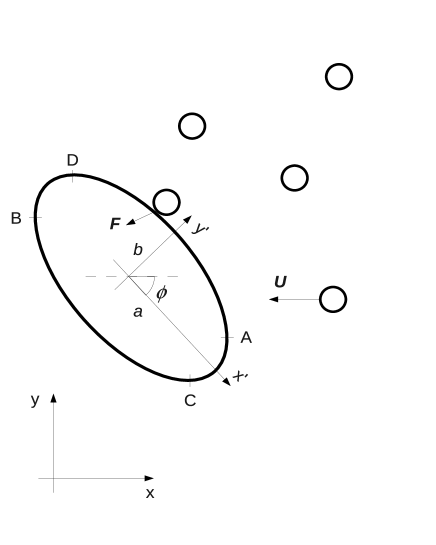
Figure 1: Ellipse’s local frame of reference (primed system), rotated an angle $\phi$ about its center. The major and minor half-axes are given by $a$ and $b$, respectively. The force ${\bf F}$ is the total (normal plus tangential) force between a disk and the obstacle. See text for the meaning of the four points $A$, $B$, $C$ and $D$.

First of all, all disks are assumed to have only the horizontal velocity component, $U$. Therefore, for the ellipse given in fig. 1, which is located at $(x_{E}$,$y_{E})$, a collision will occur only if the impact parameter (the vertical distance between a disk’s center and the horizontal line through the ellipse’s center) is in the range $\left[y_{C}+\frac{d}{2}\right.$,$\left.y_{D}+\frac{d}{2}\right]$. This is so because $C$ and $D$ are, respectively, the lowest and the highest points in the ellipse, in the same way as $A$ and $B$ are the leftmost and the rightmost ones. Any collisions that happen in the segment $\overline{AD}$ will exert a downward lift, while collisions that occur in the $\overline{AC}$ segment will produce an upward lift (from now on, the $\overline{AD}$ segment, and all other segments in the text, will be referred to only as $\overline{AD}$). Moreover, since the lengths of both segments are, in general, unequal, the longest of them, in this case $\overline{AD}$, will suffer more collisions than the other, which implies a net, negative, lift force. It is this mechanism that prevents any net lift to take place on a circular obstacle under these conditions (in general, any body that is symmetrical with respect to the flow direction, and is fully immersed in the flow, does not suffer a net lift). Therefore, the determination of the coordinates of these four points in the ellipse, $A$, $B$, $C$ and $D$, is very important.

In order to do this, one should notice that the tangent line to the ellipse is horizontal at $D$ and $C$ and vertical at $A$ and $B$. Therefore, starting from the tilted ellipse’s equation in the global frame:

$$\left(a^{2}\sin^{2}\phi+b^{2}\cos^{2}\phi\right)X^{2}+\left(a^{2}\cos^{2}\phi+b^{2}\sin^{2}\phi\right)Y^{2}-\sin 2\phi\left(a^{2}-b^{2}\right)XY=a^{2}b^{2},$$ (1)

where $X=x-x_{E}$ and $Y=y-y_{E}$, one can write for $D$ and $C$:

$$x_{D,C}=x_{E}\pm\frac{\sin\phi\cos\phi(a^{2}-b^{2})}{\sqrt{a^{2}\sin^{2}\phi+b^{2}\cos^{2}\phi}},$$ (2)

and

$$y_{D,C}=y_{E}\pm\sqrt{a^{2}\sin^{2}\phi+b^{2}\cos^{2}\phi}.$$ (3)

where the plus(minus) sign is for point $D$($C$). A similar calculation yields, for points $A$ and $B$:

$$x_{B,A}=x_{E}\pm\sqrt{a^{2}\cos^{2}\phi+b^{2}\sin^{2}\phi},$$ (4)

and

$$y_{B,A}=y_{E}\pm\frac{\sin\phi\cos\phi(a^{2}-b^{2})}{\sqrt{a^{2}\cos^{2}\phi+b^{2}\sin^{2}\phi}},$$ (5)

where in both eqs. the plus(minus) sign is for point $B$($A$).

The force due to a collision between a disk and the ellipse can be obtained by calculating the change in linear momentum of the disk. The total force is obtained by integrating the product of this individual momentum change and a suitable collision rate over the obstacle section facing the flow, i.e., integrating over $\overline{CD}$.

Suppose a disk hits the obstacle in $\overline{AD}$. Figure 2 presents schematically the geometry of the collision (assumed frictionless).

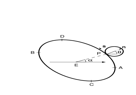
Figure 2: Geometry of the collision between a disk and the ellipse, centered at $E$. They touch each other at the point $P$ in the ellipse. $\theta$ and $\alpha$ are the impact and collision angles.

The grain velocity is ${\bf v}_{0}=-U{\bf i}$, and the impact angle is $\theta$, which is the one between the direction ${\bf i}$ and the normal at the contact point. The post-collisional velocity is ${\bf v}=v_{x}{\bf i}+v_{y}{\bf j}$. In order to obtain the final components as a function of $U$, one has two equations that relate the normal and tangential velocities before and after the collision: ${\bf v}\cdot{\bf\hat{n}}=-e{\bf v}_{0}\cdot{\bf\hat{n}}$ and ${\bf v}\cdot{\bf\hat{s}}={\bf v}_{0}\cdot{\bf\hat{s}}$, where ${\bf\hat{n}}=\cos\theta{\bf i}+\sin\theta{\bf j}$, ${\bf\hat{s}}=-\sin\theta{\bf i}+\cos\theta{\bf j}$ are the normal and tangential unit vectors at the collision point and $e$ is the normal restitution coefficient, assumed velocity independent.

From these considerations, the components of the disk velocity after the collision are $v_{x}=U(\sin^{2}\theta-e\cos^{2}\theta)$ and $v_{y}=\frac{1}{2}U(1+e)\sin 2\theta$. Therefore, the vertical momentum change for a general collision is given by:

$$\Delta P_{y}(\theta)=mv_{y}=\frac{1}{2}mU(1+e)\sin 2\theta.$$ (6)

The number of disks that strike the ellipse in a time $dt$ is given by the number of particles within the area of the parallelogram with sides $Udt$ and $ds$, this last quantity being the arc length around the collision point. Given the geometry of the collision (figure 2), the area of this parallelogram is $dA=U\cos\theta dtds$. Hence:

$$dN=\frac{4\nu}{\pi d^{2}}dA=\frac{4\nu}{\pi d^{2}}U\cos\theta dtds,$$ (7)

where $\nu$ is the area fraction of the incoming flow. The collision frequency is simply this number divided by $dt$.

The arc length $ds$ is given by the product of the collision radius, $R(\alpha)$, by the arc element, $d\alpha$. This product is readily evaluated for a circle. However, in the ellipse case, this is not so simple, since this radius varies with $\alpha$. Besides, the grain size introduces an additional complication for calculating $R(\alpha)$, as seen in fig. 3, which shows the triangle formed by the disk center, the ellipse center and the collision point.

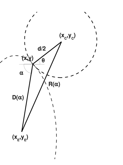
Figure 3: Triangle formed by the disk center, $(x_{C},y_{C})$, the ellipse center, $(x_{E},y_{E})$ and the collision point, $(x,y)$ (angles are exaggerated). The angle between $D(\alpha)$ and the normal to the disk center is $\pi-\alpha+\theta$. Dashed lines are sketches of the surfaces of the disk and the ellipse.

Hence, the ellipse is assumed much larger than the disks and the disk size only enters the expression for $R(\alpha)$ as a minor correction. With this assumption, the arc length is given by $ds=D(\alpha)d\alpha$. In parametric form, $x=a\cos\alpha$ and $y=b\sin\alpha$, this length reads:

$$ds=\sqrt{\left(\frac{dx}{d\alpha}\right)^{2}+\left(\frac{dy}{d\alpha}\right)^{2}}d\alpha=(\sqrt{a^{2}\cos^{2}\alpha+b^{2}\sin^{2}\alpha})d\alpha.$$

Finally, the effective collision radius is given by:

$$D(\alpha)=(a^{2}\cos^{2}\alpha+b^{2}\sin^{2}\alpha)^{1/2}.$$ (8)

Another difficulty to obtain the expression for the lift force is that the momentum change (i.e., the force) depends explicitly on $\theta$, while the collision frequency depends on $\alpha$. Therefore, any hope of integrating the lift force over all collisions should pass through obtaining the relationship between the angles $\theta$ and $\alpha$. This is done in the following paragraph.

Since $dx/dy$ gives the tangent of the angle between the normal line to a point in the ellipse and the $x$ axis, from the ellipse equation (1), one has:

$$\tan\theta=\frac{2C_{2}Y-C_{3}X}{C_{3}Y-2C_{1}X},$$

where $C_{1}$, $C_{2}$ and $C_{3}$ are the coefficients of the terms $X^{2}$, $Y^{2}$ and $XY$ in eq. (1). Since $\tan\alpha=Y/X$ and from eqs. (2), (3), (4) and (5), the relation between $\theta$ and $\alpha$ can be cast in terms of the coordinates of the points $D$ and $A$, since:

$$\tan\alpha_{D}=\frac{y_{D}-y_{E}}{x_{D}-x_{E}}=\frac{a^{2}\sin^{2}\phi+b^{2}\cos^{2}\phi}{(1/2)\sin 2\phi(a^{2}-b^{2})}=\frac{2C_{1}}{C_{3}}$$

and

$$\tan\alpha_{A}=\frac{y_{A}-y_{E}}{x_{A}-x_{E}}=\frac{(1/2)\sin\phi\cos\phi(a^{2}-b^{2})}{a^{2}\cos^{2}\phi+b^{2}\sin^{2}\phi}=\frac{C_{3}}{2C_{2}}.$$

Hence:

$$\tan\theta=\frac{1}{\tan\alpha_{A}}\frac{\tan\alpha_{A}-\tan\alpha}{\tan\alpha_{D}-\tan\alpha}.$$ (9)

The lift force can now be evaluated as:

$$L=-\int\Delta P_{y}d\dot{N}$$

where $d\dot{N}=dN/dt$. By using eqs. (6), (7) and (8), the total lift on the ellipse due to collisions is given by:

$$L=-\frac{1}{2}\rho U^{2}(1+e)\int\limits_{C}^{D}\sin 2\theta\cos\theta ds(\alpha),$$ (10)

where $\rho=4m\nu/\pi d^{2}$ is the flow mass density and the arc length is to be calculated bearing in mind (9).

II.2 Model results

The lift force scales with the obstacle size $a$, as expected, since it depends linearly on the arc length. Also, it is seen that, for more inelastic grains the lift is smaller, since more inelasticity implies less intense change of momentum, see eq. (6). The dependence of the lift on the tilt angle is hidden in the integral over $\overline{CD}$, because the lengths of $\overline{AC}$ and $\overline{AD}$, which contribute forces with distinct signs, are unequal for a general $\phi$.

Apart from the dependence of $L$ in these parameters, it also depends on the ellipse eccentricity, i.e., on the ratio of the ellipse’s axes $0\leq k=b/a\leq 1$. For $k=1$, the obstacle is a circle, and the lift vanishes by symmetry. In the other extreme value, $k=0$, which corresponds to a flat plate, the lift vanishes only for $\phi=0$ (horizontal plate) and $\phi=\pm\pi/2$ (vertical plate), which are the only symmetrical orientations with respect to an horizontal flow. In fig. 4, it is shown the predictions of eq. (10) for distinct values of $k$ (the parameter values in plotting these curves were chosen to agree with those used in the simulations).

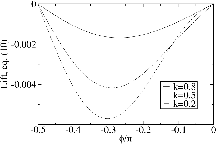
Figure 4: Eq. (10) for distinct eccentricity, $k$, values. The curves were obtained with $\nu=0.196$, $d=1$, $m=1$, $U=10$ and $e=0.952$.

One can see that the maximum (absolute) value of $L$ increases when $k$ decreases. This happens because when $k\rightarrow 0$, the points $D$ and $C$ merge with points $B$ and $A$, as can be inferred from eqs. (2), (3), (4), and (5). In this case, $\overline{AD}\rightarrow 2a$ and $\overline{AC}\rightarrow 0$. Since the lift is the difference of the contributions from $\overline{AD}$ and $\overline{AC}$, all collisions will give positive contributions to the net lift value, and it should reach its maximum for a particular $\phi$.

The objective of the simulations is to study the lift force on the obstacle as a function of four parameters that appear on eq. (10), namely, the obstacle size, $a$, the restitution coefficient, $e$, the ellipse eccentricity, $k$, and the tilt angle, $\phi$.

III Simulation

In this section, the simulation is detailed, along with the parameter values used in the computations, and the numerical results for the lift are shown.

III.1 Design

The system is composed of $N$ soft disks, with unity diameter $d$ and unity mass $m$, located in a workspace of lengths $L_{X}$ and $L_{Y}$ in the horizontal and vertical directions, respectively. They interact through normal and tangential forces, according to the model used in rapaport ; Ciamarra04 . The normal force between two disks is:

$${\bf F}_{ij}^{N}={\bf f}_{ij}+{\bf f}_{ij}^{d},$$ (11)

where the first term is the conservative part, given by a simple harmonic spring force

$${\bf f}_{ij}=\kappa\left(\frac{d_{i}+d_{j}}{2}-r_{ij}\right){\bf{\hat{r}}}_{ij},$$

where $\kappa$ is the spring constant, $d_{i}$ is the $i$-th disk diameter, $r_{ij}$ is the distance between the two disks and ${\bf{\hat{r}}}_{ij}$ is a unit vector along the normal between the disks’ centers. The second term is a dissipative, velocity dependent force, given by

$${\bf f}_{ij}^{d}=-\gamma_{d}({\bf{\hat{r}}}_{ij}\cdot{\bf v}_{ij}){\bf{\hat{r}}}_{ij},$$

where $\gamma_{d}$ is the normal damping coefficient and ${\bf v}_{ij}={\bf v}_{i}-{\bf v}_{j}$ is the relative velocity between the contacting disks. The tangential force at the contact point is given by the following expression:

$${\bf F}_{ij}^{S}=-\min\left(\gamma_{s}v_{ij}^{S},\mu F_{N}\right){\bf{\hat{v}}}_{ij}^{S},$$ (12)

where $\gamma_{s}$ is the sliding friction constant and $\mu$, the static friction coefficient, while ${\bf{\hat{v}}}_{ij}^{S}$ is the unit vector along the direction of the relative velocity at the contact point. This vector is calculated as:

$${\bf v}_{ij}^{S}={\bf v}_{ij}-({\bf{\hat{r}}}_{ij}\cdot{\bf v}_{ij}){\bf{\hat{r}}}_{ij}-\left(\frac{{\bm{\omega}}_{i}+{\bm{\omega}}_{j}}{2}\right)\times{\bf r}_{ij},$$

where ${\bm{\omega}}_{i}$ is the $i$-th disk angular velocity and $v_{ij}^{S}=\left|{\bf v}_{ij}^{S}\right|$. The total contact force ${\bf F}_{ij}={\bf F}_{ij}^{N}+{\bf F}_{ij}^{S}$ vanishes if the disks are not in contact, i.e., if $\frac{d_{i}+d_{j}}{2}>r_{ij}$.

The values of the elastic parameters used were: $\kappa=50000$, $\gamma_{d}=10$ and $\gamma_{d}=100$, $\gamma_{s}=0.1$ and $\mu=1$. The restitution coefficient Silbert01 for these parameters were $e=0.952$, for $\gamma_{d}=10$, and $e=0.608$, for $\gamma_{d}=100$. The ellipse’s major and minor half-axes are $a$ and $b=ka$, respectively. The parameter $a$ has the values $5$, $10$, $20$, $30$ and $40$, with $k=0.8$. For the studies of the dependence on $k$, size $a=10$ was used, with $k=0.80$, $0.50$ and $0.20$. All these cases were studied for both $e$ values. For the two smaller obstacle sizes, results were obtained with a $N=2500$ and $L_{X}=L_{Y}=100$ packing, while for the others, a $N=10000$ and $L_{X}=L_{Y}=200$ packing was used. In both cases, the packing fraction was about $0.200$. The ellipse is located in $x_{E}=0.5L_{X}$ and $y_{E}=0.5L_{Y}$, and its major half-axis is tilted related to the horizontal axis (flow direction) by $\phi$. The values of the tilt angle were in the range $[-\pi/2$,$0]$, divided in $\pi/20$ increments, which gives a total of $11$ distinct $\phi$ values.

At the beginning, all disks are randomly generated without overlap among them and the ellipse. At this stage, the obstacle is modeled as a circle with diameter $2a$ since this facilitates the overlap check. All disks have initial velocity ${\bf v}_{0}=-U{\bf i}$, where ${\bf i}$ is the unit vector in the horizontal (flow) direction and $U=10$.

The system has periodic boundaries perpendicular to the flow direction, while, along the flow, the conditions are the same as in Wass03 : whenever a disk leaves the system through the right boundary, it is placed at the left one in a random vertical position. In fact, the code searches for a position where the incoming grain overlaps with no other disk, which is fairly easy, giving the low density that is used here. Its velocity is set as the incoming flow velocity ${\bf v}_{0}$ plus a small random vertical component chosen uniformly in the interval $[-fU,fU]$, where $f=0.10$ (results obtained with $f=0$ differ little from those shown here).

The interactions between the disks and the ellipse are the same as those given above for two disks. The main problem is to resolve particle-ellipse contacts. In order to do this, all disks are checked for overlap with a circle of diameter $2a$. If one disk overlaps with the circle, it is mapped in the ellipse’s local frame of reference (ELFR). Then, the contact point coordinates, in the ELFR, are calculated using the algorithm proposed in Dziu01 . The direction of the normal force is along the line joining the disk center and the contact point, while the tangential force is perpendicular to this direction.

Lengths, forces and time are given in units of $d$, $\kappa d$, and $\sqrt{m/\kappa}$, respectively. Equations of motion are integrated with a leapfrog scheme rapaport , with a time step of $0.001$. Each simulation is performed during $10^{5}$ molecular dynamics (MD) cycles for thermalization and $10^{6}$ MD cycles for measurements. All results are averaged over $20$ and $10$ independent runs for the $N=2500$ and $N=10000$ packings, respectively.

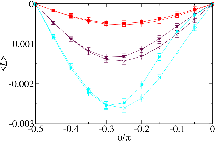
Figure 5: (Color online) Lift as a function of eccentricity, $k$, restitution coefficient and tilt angle, $\phi$. Squares represent $k=0.80$ results, inverted triangles, $k=0.50$ and left triangles, $k=0.20$. Open and filled symbols are for $e=0.952$ and $0.608$. All results are for $a=10$. Lines are only guides to the eyes.

The main interest is to measure the force exerted on the obstacle by the stream of grains due to the collisions among them. Therefore, the components of this force, drag and lift, are measured at all cycles after thermalization. At regular intervals, the forces are recorded as averages over this period. This accumulation interval is $1000$ MD cycles long (results were also obtained with $10000$ MD cycles long accumulation periods and do not differ appreciably from those reported here). The flow velocity and particle number density fields, ${\bf v}(x,y)$ and $\rho(x,y)$, were measured as follows: the workspace is divided in square bins of side $d$. At each cycle, all particles are mapped in an appropriate bin and its velocity components are added to the respective field element. Similarly, angular profiles related to the contact angle between the grains and the ellipse, the collision angle $\alpha$, were measured. They are the collision number and the velocity components. Each time there is a disk-ellipse contact, the angle formed by the line joining the collision point and the ellipse center with the flow direction is calculated. Then, the above mentioned quantities are added to the appropriate profile bins. The field and the profiles are presented as averages over cycles and runs.

III.2 Results

In fig. 5, the numerical results for the lift as a function of the tilt angle and the eccentricity are shown.

Comparing figs. 4 and 5, it is clear that eq. (10) captures the qualitative features of the lift force, even though the correspondence becomes weak for $k=0.20$ and $e=0.952$. Also, the results agree with the prediction that the lift should be higher for less inelastic flows. Finally, the theoretical result overestimates the numerical ones by, roughly, a factor of $2$, for these cases.

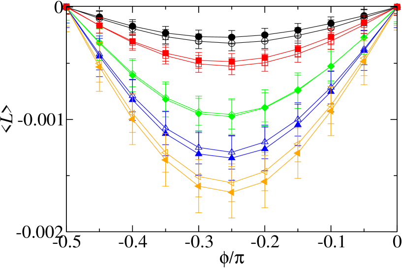
Figure 6: (Color online) Lift force as a function of the tilt angle, obstacle size, $a$, and restitution coefficient $e$. Distinct symbols are $a=5$ (black circles), $a=10$ (red squares), $a=20$ (green diamonds), $a=30$ (blue triangles) and $a=40$ (orange left triangles). All are for $k=0.80$. Open and filled symbols are results for $e=0.952$ and $e=0.608$, respectively. Lines are only guides to the eyes.

In fig. 6, the numerical results for the lift force as a function of the tilt angle and obstacle size are shown. As expected, the lift increases with the obstacle size. However, the lift does not grow linearly with $a$. Plotting these data against the obstacle size shows that $\left<L\right>\sim a^{0.78(2)}$. Since the results are not conclusive, it suffices to acknowledge that more simulations are needed in order to obtain a more reliable scaling with the obstacle size. Also, this figure shows that the lift force for $e=0.608$ packings grows faster with $a$ than for those with $e=0.952$. Finally, the numerical results, as seen in fig. 5, also are smaller than their theoretical counterparts (for $a=40$, the factor is about $4$). This shows that the difference between model and theory depends only a little on the tilt angle, while the obstacle size, inelasticity and eccentricity are the factors that accept the most on this difference.

The reasons behind the failure to reproduce the numerical results will be analyzed in the next section, where the assumption that led to eq. (10) will be reviewed in detail.

IV Analyses

There are three basic hypotheses on which the argument for the lift force in section II.1 was built. The first one is that particle-obstacle interactions were frictionless, despite the force model, eq. (12), is not. Second, the arc length expression, $ds=D(\alpha)d\alpha$, does not take into account the fact that the grains have a finite diameter $d$. Finally, the collision frequency expression (7) was obtained under the hypothesis that only one particle at a time hits the obstacle, i.e., a disk-ellipse collision does not affect the next collision, a condition met only in very dilute or in ideal gas flows (which is not the case here). Therefore, its applicability here is clearly questionable, as inferred from the system configuration shown in fig. 7.

Figure 7: System configuration. Parameters: $a=40$, $k=0.80$, $e=0.952$ and $\phi=-\pi/4$.

There is a dense region that begins above point $A$ and forms a separation boundary in front of the ellipse. This is the typical granular shock wave Amar01 ; Rericha02 ; Boudet08 ; Buchholtz98 ; Wass03 that forms around bodies immersed in fast granular flows. Clearly, the dilute flow assumption is not valid. Figure 8 shows the clear signature of this structure in the velocity field.

Also, this picture shows that the two branches of the shock wave meet behind the obstacle. This fact could, at first sight, invalidates the lift results because this clearly does not allow the use of periodic boundaries perpendicular to the stream. This is not the case, however, as seen in the results for the lift obtained from simulations that used rigid walls in the $y$ direction. These results agree with those shown in figs. 5 and 6 within numerical error. Nevertheless, periodic boundaries in a particular direction should only be used when the system is independent in that direction.

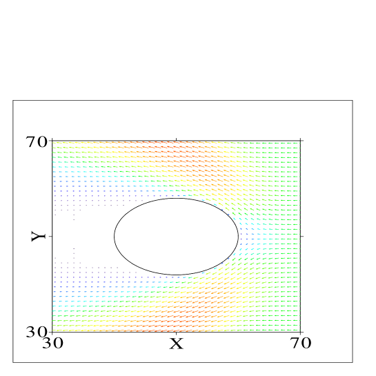
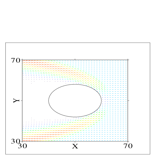
Figure 8: (Color online) Velocity fields detailed around the obstacle for $a=10$, $k=0.80$, $\phi=0$, $e=0.952$ (top) and $e=0.608$ (bottom).

Before discussing the influence of the shock wave in the results, a few brief comments will be made regarding the first two assumptions in the theoretical argument.

To take into account the grain size in computing the collision radius is to consider a larger (effective) obstacle facing the flow, which would increase the theoretical prediction for the lift. Since this quantity is already larger than the numerical results, it was safe to ignore it in the calculations.

The influence of the friction force on the lift can be inferred from the velocity field results, fig. 8. As seen in this figure, particles follow tangential trajectories along the ellipse Amar01 ; Rericha02 ; Boudet08 , which means that they slide along the obstacle. Since friction is a tangential force, one concludes that a grain sliding along $\overline{AD}$ exerts an upward lift. By symmetry, a disk exerts a downward lift while sliding along $\overline{AC}$. Therefore, the net effect of friction is to decrease the lift exerted by collisions in each segment. The combination of both effects might decrease or increase the net lift. The numerical results for the lift rising from friction show that it is opposite to the one resulting from the normal force. In other words, friction decreases the net lift. The effect is small, though, because the sliding friction is also small, $\gamma_{s}=0.1$. In most simulations of granular matter, regardless of the tangential force model, the sliding friction is only mildly lower than the normal interaction parameter. Here, a much lower value was used, which could greatly affect the results. Simulations performed with a distinct set of parameters, $\gamma_{s}=5000$ and $\mu=0.1$, values which are more common to general simulations of granular matter, show that the results do not change significantly, and are still qualitatively the same as those in figs. 5 and 6. In fact, the lift data are reduced only by $5\%$ to $10\%$. This happens due to the fact that the velocities involved in the simulations are high enough for the tangential force to reach the Coulomb static friction criterion, which caps its maximum value and limits its influence on the lift. This conclusion is supported by the fact that the fraction of all disk-obstacle contacts, for $\gamma_{s}=5000$, that reach the failure condition is about $99.5\%$, with only a very small $\phi$ dependence.

As stated earlier, the dilute flow assumption does not hold. A rigorous calculation of the force in the obstacle, in which all dense packing effects are taken into account, is not a simple matter. In Deng10 an attempt was made in this direction. The formation of the shock wave produces a dense region that shields the obstacle from the incoming particles. Since the interactions are dissipative, particles should reach the obstacle with reduced velocities. This clearly reduces the force exerted by the disks. Also, given the large density within the shock wave, the collision rate might be affected. Finally, as seen from the velocity field data, fig. 8, particles should hit the obstacle, on average, with a non vanishing vertical velocity component, i.e., particles suffer oblique inelastic collisions, which could affect the force on the obstacle. Both effects will be discussed in more detail in the following two subsections. This discussion will by made only qualitatively, since more simulations are needed to determine the amount of influence each of them has on the results.

IV.1 Obstacle shielding

One of the consequences of the existence of the shock wave is that the obstacle is shielded from the flow, in a way that the grains hit it with lower horizontal velocity than the upflow value. This fact alone indicates that the numerical net lift should be lower than its theoretical prediction. Aside from reducing the incoming flow velocity, the shock wave forms a dense region around the obstacle through which grains should go through in order to reach it. This could affect the collision rate and, in turn, the net lift. Both effects must play a role in order to explain the faster growth of the lift force with the obstacle size for stronger inelasticity flow compared to that of lower inelasticity one.

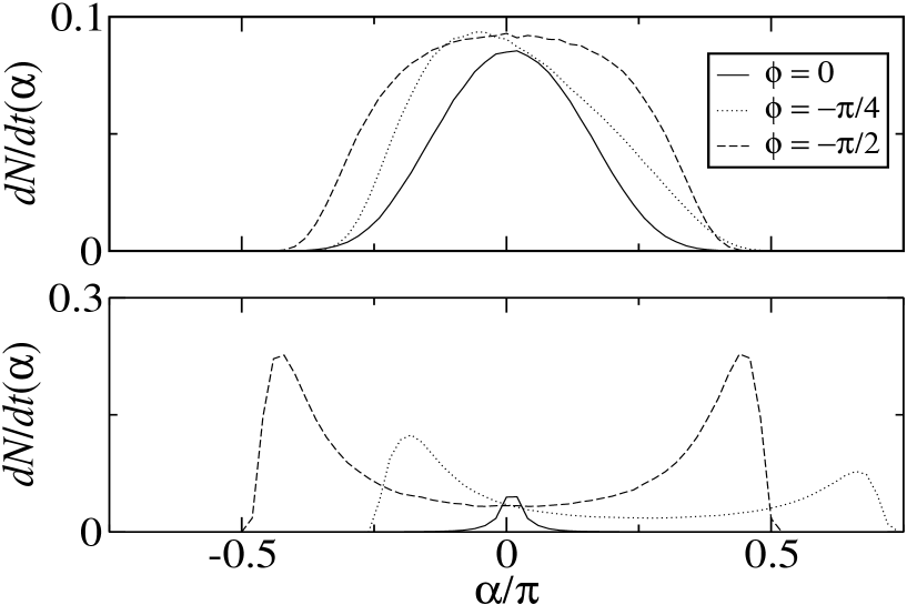
Figure 9: Angular collision profiles, for $a=10$, $e=0.608$, $k=0.80$ (upper row) and $k=0.20$ (lower row), for three distinct tilt angles (shown in the legend box). The horizontal scales are the same for both plots.

The results for the collision profiles show that, for $e=0.608$, the shock wave is more localized around point $A$ (where, for the $k=0.80$ obstacles the peak of the profiles is located) and that the overall collision number is greatly increased compared to the number when $e=0.952$. This is a consequence of the aggregation that grains suffer due to the inelastic interactions and is common to all cases studied. This fact implies that the force on the obstacle should increase due to this increase in the collision rate and could compensate, in part, for the decrease in the force due to the reduced incoming velocity.

The collision profiles are changed, in a very different way, for obstacles with distinct eccentricities, $k$. Fig. 9 has results that illustrate this effect. The most striking feature of these curves is that the profiles for $k=0.20$ develop two peaks, instead of the more familiar one around point $A$, which is still present, but it moves away from this point as the ellipse is oriented vertically. The other one develops around point $D$ and is seen at tilt angles as high as $\phi=-\pi/10$. Such features are also seen in the $k=0.50$ results, although with smaller peaks. These results can be explained by the fact that in some cases, for stream velocities below a critical value, there is the appearance of a gap, filled with a hot granular gas, between the obstacle and the shock wave Buchholtz98 . In the present case, the appearance of the gap is a function of $k$ alone, since the stream velocity is the same for all simulations. Figure 10 has a result for the density field that indicates the presence of the gap. Notice the denser arc formed right in front of the ellipse, the region limited by this arc and the obstacle is the gap.

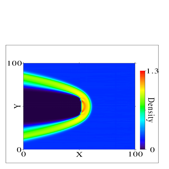
Figure 10: (Color online) Density field for $a=10$, $e=0.608$, $k=0.80$ and $\phi=-\pi/2$. The gap is the yellow (white) region between the red (light gray) arch and the ellipse (not shown).

As a last note, the collision rate increases faster with $\phi$ for $k=0.20$ than for $k=0.80$. Fig. 11 has two configuration snapshots that illustrate the shock wave for two obstacles with distinct eccentricities.

Figure 11: Two packing configurations for $a=10$, $\phi=-\pi/4$, $e=0.608$ and $k=0.80$ (top) and $k=0.20$ (bottom).

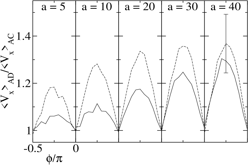
Figure 12: Ratio between the average horizontal velocity components in $\overline{AD}$ and $\overline{AC}$ for obstacles with $k=0.80$. Full lines correspond to packings with $e=0.952$, while dashed lines, to $e=0.608$. Scales in all plots are the same.

One can infer from these pictures the reason behind the asymmetrical peaks in the collision profiles when $\phi=-\pi/4$ and $k=0.20$. There is a very small concentration of particles in front of $\overline{AC}$, which certainly allows for more collisions to occur.

These considerations still left unanswered the question about the faster growth of $\left<L\right>$ with $a$ for stronger inelasticity compared to those at lower inelasticity. Since the net lift is the difference of the forces exerted in $\overline{AC}$ and $\overline{AD}$, one should seek a relative measure of the speeds in each of them in order to account for the size of the contributions each has in the net value. This is done by calculating the ratio between the average horizontal disk velocities in $\overline{AD}$ and $\overline{AC}$. If this ratio is greater than $1$, the collisions on $\overline{AD}$ exert, on average, a stronger force than those on $\overline{AC}$. These averages are evaluated directly from the simulations. The results, for all tilt angles and obstacle sizes, are given in fig. 12.

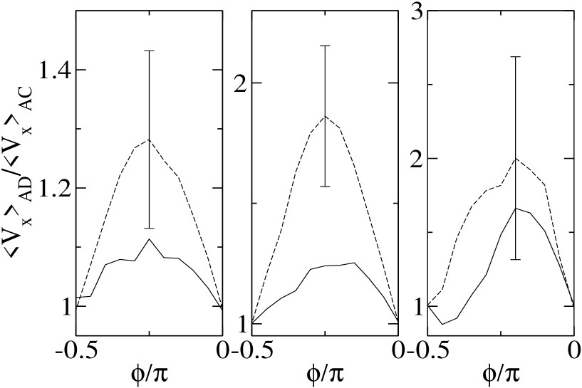
Figure 13: Ratio between the average horizontal velocity components in $\overline{AD}$ and $\overline{AC}$ for obstacles with $k=0.80$ (left panel), $k=0.50$ (middle panel) and $k=0.20$ (right panel). Full lines correspond to packings with $e=0.952$, while dashed lines, to $e=0.608$.

First it can be seen that except in a few cases, markedly at small obstacles, all ratios are larger than $1$, and those for $e=0.608$ cases are larger than those for $0.952$. It is possible to identify a trend in these graphs, despite the noise: the ratio grows with obstacle size. This is consistent with the results in fig. 6, where the net lift grows faster with $a$ for the $e=0.608$ flows compared to those with $e=0.952$. Fig. 13 has the data for the same quantity measured for obstacles with distinct eccentricities.

It is seen that the ratio increases as $k$ decreases (it reaches a factor of $2$ for $k=0.20$). These data, together with those for the collision profiles, show that the large lift observed for low $k$ obstacles is a consequence not only of a larger number of collisions at $\overline{AD}$, but also due to collisions with larger speeds than those at $\overline{AC}$.

IV.2 Oblique impacts

The last piece of this analysis is the role of the vertical velocity component in the lift value. Before proceeding, the collision argument of section II is reviewed by allowing the incoming disks to have a vertical velocity, $V$, and calculating the new momentum change in each collision. This will elucidate the effect of the vertical velocity on the lift value.

The velocity of a disk which collides with the obstacle is ${\bf v}_{0}=-U{\bf i}+V{\bf j}$. The final disk velocity for a inelastic, frictionless collision is obtained as:

$$v_{x}=U(e\cos^{2}\theta-\sin^{2}\theta)-\frac{1}{2}V(1+e)\sin 2\theta,$$ (13)

and

$$v_{y}=\frac{1}{2}U(1+e)\sin 2\theta+V(\cos^{2}\theta-e\sin^{2}\theta).$$ (14)

The vertical momentum change due to this collision is given by:

$$\Delta P_{y}=m(v_{y}-V),$$

using the result for $v_{y}$, (14), and performing some algebra, the new momentum change is:

$$\Delta P_{y}=m(1+e)\left[\frac{1}{2}U\sin 2\theta-V\sin^{2}\theta\right],$$ (15)

where $U>0$.

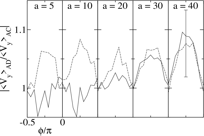
Figure 14: Ratio between the average vertical velocity components in $\overline{AD}$ and $\overline{AC}$. Full lines correspond to packings with $e=0.952$, while dashed lines, to $e=0.608$. Scales in all plots are the same.

By looking at eq. (15) one can see that a collision that happens in the range $-\pi/2<\theta<0$, which corresponds to $\overline{AC}$, will produce a lower momentum change if $V<0$. Similarly, for collisions that take place in the range $0<\theta<\pi/2$, which is $\overline{AD}$, a lower momentum change will occur if $V>0$. From the velocity field data, fig. 8, it is clear that the average vertical velocities in $\overline{AD}$ and $\overline{AC}$ are positive and negative, respectively. The oblique impacts decrease the positive lift exerted by the flow in $\overline{AC}$, but also decrease the negative lift in $\overline{AD}$. Therefore, it is not obvious if both effects combined increase or decrease the net lift. In order for this combination of effects to increase the net lift, the vertical velocity in $\overline{AD}$ should be lower than the corresponding velocity in $\overline{AC}$. In figs. 14 and 15, the absolute value of the ratio of the average vertical velocities in both segments is shown for distinct obstacle sizes eccentricities, respectively.

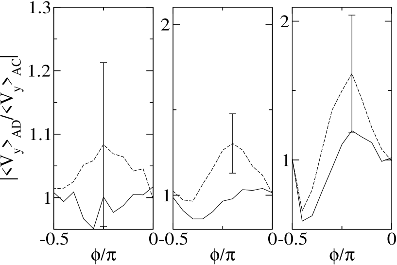
Figure 15: Ratio between the average vertical velocity components in $\overline{AD}$ and $\overline{AC}$. Full lines correspond to packings with $e=0.952$, while dashed lines, to $e=0.608$. The left panel is for $k=0.80$, the middle one, for $k=0.50$ and the right one, for $k=0.20$.

It is seen that the ratio, for $e=0.608$, depends little on the obstacle size and restitution coefficient, and that those for $e=0.952$ grow with $a$. It varies strongly with tile angle and eccentricity. Despite a few cases, the ratio is larger than $1$ which implies that the net lift decreases due to oblique impacts, as provided by the existence of the shock wave.

V Conclusions

A theoretical argument and numerical results on the net lift force exerted by a granular stream of equal disks on an ellipse were presented. The argument used to obtain a theoretical expression for the lift relied on inelastic, frictionless collisions of a very dilute granular flow, in the horizontal direction, and the ellipse. The expression obtained, eq. (10), captures nicely the qualitative features of the numerical results. It does not, however, reproduce the results quantitatively, neither does it reproduce the difference in the lift force for $e=0.952$ and $e=0.608$.

The numerical data, shown in figs. 5 and 6, are lower than the theoretical prediction by a factor that depends mostly on the obstacle size (for $a=40$, eq. (10) is about $4$ times larger than the measured results).

Additional analyses of the flow properties showed that, from the assumptions drawn in the text, the dilute flow one is the most problematic. The existence of the granular shock wave Amar01 ; Rericha02 ; Boudet08 ; Buchholtz98 ; Wass03 invalidates this hypothesis. This structure affects directly the velocity components of the disks at contact with the obstacle as well as the collision rate. The horizontal velocity at contact decreases due to dissipative collisions that occur before the disks reach the shock wave. Also, some of the horizontal momentum is deviated by the shock wave around the obstacle, introducing a vertical component whose net effect is to decrease the lift.

Perspectives to this work include a deeper analysis of dense packing effects on the lift. This would answer questions about the scaling of the lift with obstacle size, flow speed and density. Such analysis would also allows for a better understanding of the mechanism behind the appearance of the net lift, since an obvious consequence of the presence of the shock wave is that any collisions that occur on its edge should transmit some linear momentum through the dense region until pushing the disks closets to the obstacle, and that is when the actual force is made. Force transmission models, such as those in Liu95 ; Ostojic05 can be good starting points for this analysis. Moreover, the effect of eccentricity on the shock wave is something worth investigating since, as seen here, for a constant flow speed, there should be some eccentricity value that allows for the appearance of the gap between the shock wave and the obstacle. Finally, the hydrodynamical approach to granular flow could also be tested in such a situation. As argued in the text, ignoring the disk size does not affect the results for large obstacles. Hence, if the obstacle is much larger than the disks, the predictions of such theory should be realized in simulations, since scale separation could be achieved, at least approximately.

References

- (1) H. M. Jaeger, S. R. Nagel, R. P. Behringer, Rev. Mod. Phys. 68, 1259 (1996).
- (2) K. Wieghardt, Annu. Rev. Fluid Mech. 7, 89 (1975).
- (3) C. S. Campbell, Annu. Rev. Fluid Mech. 22, 57 (1990).
- (4) I. Goldhirsch, Annu. Rev. Fluid Mech. 35, 267 (2003).
- (5) GDR MiDi, Eur. Phys. J. E 14, 41 (2004).
- (6) Y. Amarouchene, J. F. Boudet, H. Kellay, Phys. Rev. Lett. 86, 4286 (2001).
- (7) E. C. Rericha, C. Bizon, M. D. Shattuck, H. L. Swinney, Phys. Rev. Lett. 88, 014302 (2002).
- (8) J. F. Boudet, Y. Amarouchene, H. Kellay, Phys. Rev. Lett. 101, 254503 (2008).
- (9) R. Albert, M. A. Pfeifer, A.-L. Barabasi, P. Schiffer, Phys. Rev. Lett. 82, 205 (1999).
- (10) D. Chehata, R. Zenit, C. R. Wassgren, Phys. Fluids 15, 1622 (2003).
- (11) V. Buchholtz, T. Poeschel, Granular Matter 1, 33 (1998).
- (12) C. R. Wassgren, J. A. Cordova, R. Zenit, A. Karion, Phys. Fluids 15, 3318 (2003).
- (13) Pica Ciamarra M. et al., Phys. Rev. Lett. 92, 194301 (2004).
- (14) R. Soller, S. A. Koehler, Phys. Rev. E 74, 021305 (2006).
- (15) Y. Ding, N. Gravish, D. I. Goldman, Phys. Rev. Lett. 106, 028001 (2011).
- (16) D. C. Rapaport, The art of molecular dynamics simulation, 2nd ed., Cambridge University Press (Cambridge, 2007).
- (17) L. E. Silbert et al., Phys. Rev. E 64, 051302 (2001).
- (18) A. Dziugys, B. Peters, Int. J. Numer. Anal. Meth. Geomech. 25, 1487 (2001).
- (19) W. H. Press, B. P. Flannery, S. A. Teukolsky, W. T. Vetterling, Numerical recipes in C, 2nd edition, Cambridge University Press (Cambridge, 1986).
- (20) Y. H. Deng, J. J. Wylie, Q. Zhang, Phys. Rev. E 82, 011307 (2010).
- (21) C.-h. Liu et al., Science 269, 513 (1995).
- (22) S. Ostojic, D. Panja, Europhys. Lett. 71, 70 (2005).