Coulomb correlations effects on localized charge relaxation in the coupled quantum dots

Abstract

We analyzed localized charge time evolution in the system of two interacting quantum dots (QD) (artificial molecule) coupled with the continuous spectrum states. We demonstrated that Coulomb interaction modifies relaxation rates and is responsible for non-monotonic time evolution of the localized charge. We suggested new mechanism of this non-monotonic charge time evolution connected with charge redistribution between different relaxation channels in each QD.

I Introduction

QDs are unique engineered small conductive regions in the semiconductor with a variable number of strongly interacting electrons which occupy well-defined discrete quantum states, for this reason they are referred to as ”artificial” atoms Kastner ,Ashoori . Several coupled QDs form an ”artificial” molecule Oosterkamp ,Blick_0 and can be applied for electronic devices creation dealing with quantum kinetics of individual localized states Stafford_0 ,Hazelzet ,Cota . That’s why the behavior of coupled QDs systems in different configurations is under careful experimental Waugh ,Blick and theoretical investigation Stafford ,Matveev . It was demonstrated experimentally that coupled QDs can vary from the weak tunneling regime (coupling with the leads is smaller than interaction between the QDs) to the strong tunneling regime (interaction with the leads exceeds the QDs coupling) Oosterkamp ,Livermore . One of the most perspective technological goals of QDs integration in a little quantum circuits deals with careful analysis of non-equilibrium charge distribution, relaxation processes and non-stationary effects influence on the electron transport through the system of QDs Angus ,Grove-Rasmussen ,Moriyama ,Landauer ,Loss . Electron transport in such systems is governed by Coulomb interaction between localized electrons and of course by the ratio between the tunneling transfer amplitudes and the QDs coupling. Correct interpretation of quantum effects in nanoscale systems gives an opportunity to create high speed electronic and logic devices Tan ,Hollenberg . So the problem of charge relaxation due to the tunneling processes between QDs coupled with the continuous spectrum states in the presence or absence of Coulomb interaction is really vital. Time evolution of charge states in a semiconductor double quantum well in the presence of Coulomb interaction was experimentally investigated in Hayashi . Authors manipulated the localized charge by the initial pulses and observed pulse-induced tunneling electrons oscillations which were fitted well by an exponential decay of the cosine function and a linearly decreasing term. Time dependence of the accumulated charge and the tunneling current through the single and coupled quantum wells in the absence of the Coulomb interaction were theoretically analyzed in Bar-Joseph , Gurvitz_1 , Gurvitz_2 . But the authors took into account only two time scales which determine charge relaxation and neglected the third time scale which is responsible for charge redistribution between different quantum wells.

In this paper we consider charge relaxation in a single QD and double QDs due to the coupling with the continuous spectrum states. In the case of two coupled QDs tunneling to the continuum is possible only from one of the QDs. We have found that on-site Coulomb repulsion even in one of the dots results in significant changing of the localized charge relaxation and leads to formation of several time ranges with strongly different values of the relaxation rates. We pointed out that the leading mechanism of non-monotonic charge relaxation is charge redistribution between the relaxation channels in one of the QDs due to the Coulomb interaction.

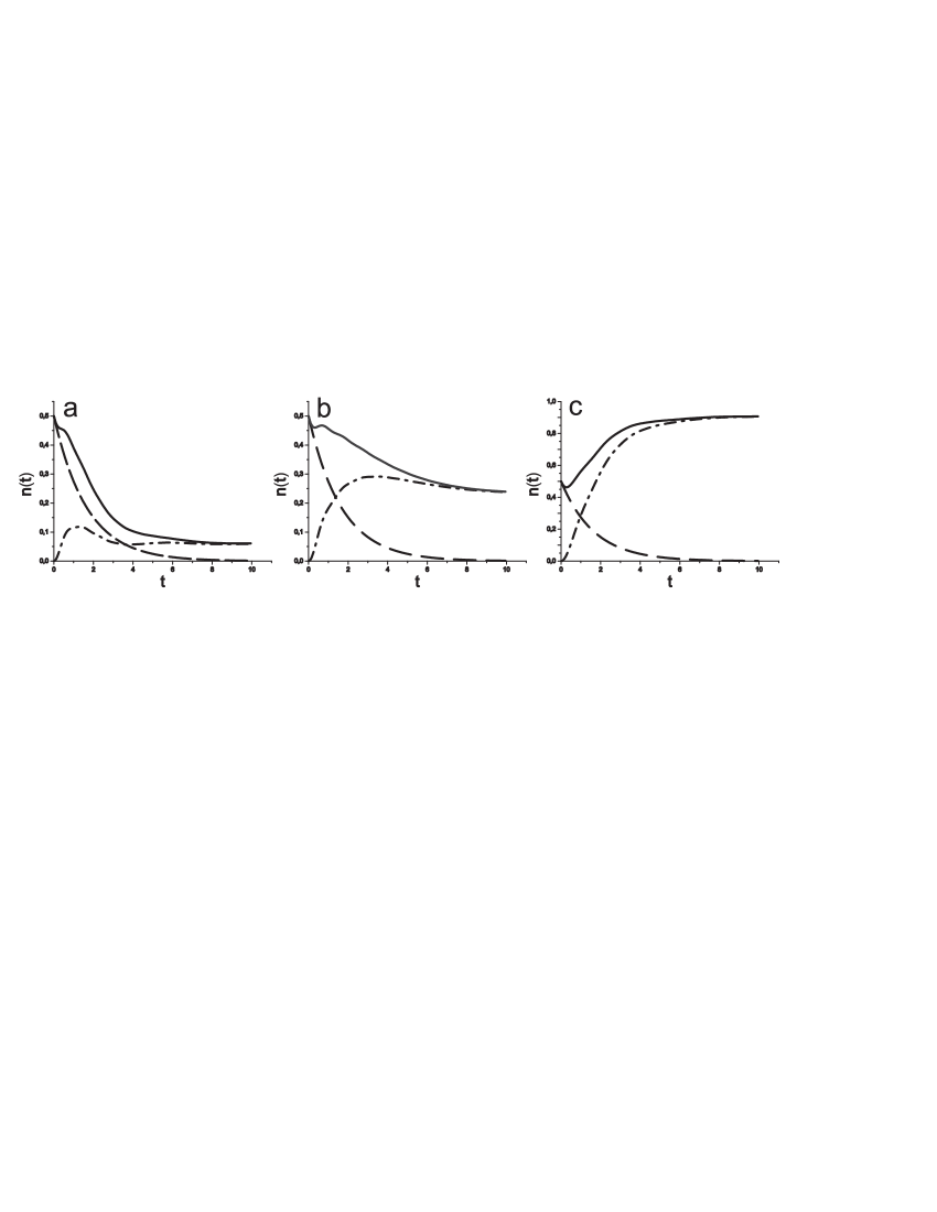
Figure 1: Solid line: Localized state filling numbers time evolution in the QD with energy level $\varepsilon_{1}$ when distribution function of the continuous spectrum electrons is taken into account. Dashed line: Filling numbers time evolution in the QD with energy level $\varepsilon_{1}$ without contribution from the conduction electrons many-particle effects. Dash-dotted line: Filling numbers evolution only due to the many particle effects caused by the presence of the distribution function. Tunneling transfer rate $\gamma_{1}=0.3$ has the same value for all the figures. a) $\varepsilon_{1}=1.3$, b) $\varepsilon_{1}=0.3$, c) $\varepsilon_{1}=-1.3$.

II Non-stationary tunneling processes in the single QD

First of all let us consider QD coupled to an electronic reservoir (conduction electrons states have energies $\varepsilon_{k}$). We assume that the single particle level spacing in the dot is larger than all other energy scales, so that only one, spin-degenerate level of the QD spectrum is accessible $\varepsilon_{1}$. Such a system can be described by the Hamiltonian:

$$\hat{H} = \sum_{\sigma}\varepsilon_{1}c_{1\sigma}^{+}c_{1\sigma}+\sum_{k,\sigma}\varepsilon_{k}c_{k\sigma}^{+}c_{k\sigma}+$$ (1)

$$+ \sum_{k,\sigma}T_{k}(c_{k\sigma}^{+}c_{1\sigma}+c_{1\sigma}^{+}c_{k\sigma})$$

where $T_{k}$ is a tunneling amplitude between the QD and the continuous spectrum states which we assume to be independent of momentum and spin. $c_{1}^{+}/c_{1}$ and $c_{k}^{+}/c_{k}$- electron creation/annihilation operators in the QD localized state and in the continuous spectrum states ($k$) correspondingly.

Let us assume that at the initial moment all charge density in the system is localized in the QD and has the value $n_{1}(0)=n_{0}$. We shall use Keldysh diagram technique Keldysh to describe charge density relaxation processes in the considered system. Time evolution of the electron density in the QD is determined by the Keldysh Green function $G_{11}^{<}$ which is connected with the localized state filling numbers in the following way:

$$G_{11}^{<}(t,t)=in_{1}(t)$$ (2)

System of integro-differential equations for the Green function $G_{11}^{<}(t,t^{{}^{\prime}})$ has the form:

$$G_{11}^{0R-1}G_{11}^{<}=\sum_{k}T_{k}G_{k1}^{<}$$

$$G_{k1}^{<}=G_{kk}^{0<}T_{k}G_{11}^{A}+G_{kk}^{0R}T_{k}G_{11}^{<}$$

(3)

and consequently one can obtain the following equation

$$(G_{11}^{0R-1}-\sum_{k}T_{k}^{2}G_{kk}^{0R})G_{11}^{<}=\sum_{k}T_{k}^{2}G_{kk}^{0<}G_{11}^{A}$$

(4)

where continuous spectrum states Green function $G_{kk}^{0R}(t,t^{{}^{\prime}})$ and inverse localized state Green function $G_{11}^{0R-1}$ in the absence of tunneling processes have the form:

$$G_{kk}^{0R}(t,t^{{}^{\prime}}) = -i\Theta(t-t^{{}^{\prime}})e^{-i\varepsilon_{k}(t-t^{{}^{\prime}})}$$

$$G_{11}^{0R-1} = i\frac{\partial}{\partial t}-\varepsilon_{1}$$ (5)

In equations (3) and (4) integration over intermediate time arguments is performed. Finally the solution of equation (4) can be written as:

$$G_{11}^{<}(t,t) = n_{1}(0)e^{-2\gamma_{1}t}+\sum_{k}\int_{0}^{t}\int_{0}^{t}\Theta(t-t_{1})\Theta(t-t_{2})\cdot$$

$$\cdot dt_{1}dt_{2}f(\varepsilon_{k})e^{-i\varepsilon_{k}(t_{1}-t_{2})}\cdot e^{-i\widetilde{\varepsilon_{1}}(t-t_{1})}e^{i\widetilde{\varepsilon_{1}}^{*}(t-t_{2})}$$

where we define

$$\widetilde{\varepsilon_{1}}=\varepsilon_{1}-i\gamma_{1}$$ (7)

and

$$\sum_{k}T_{k}^{2}G_{kk}^{0R}=-i\gamma_{1}=-i\pi T_{k}^{2}\nu_{k}^{0}$$ (8)

$\nu_{k}^{0}$-continuous spectrum density of states which is not a function of energy, $f(\omega)$-Fermi distribution function.

Performing integration in expression (LABEL:solution) and replacing summation over $k$ by integration over $\omega$ one can get final expression which describe filling numbers evolution in the quantum dot due to the interaction with the continuous spectrum states:

$$n_{1}(t) = n_{1}(0)\cdot e^{-2\gamma_{1}t}+\frac{1}{\pi}\int d\omega\cdot f(\omega)\frac{\gamma_{1}}{(\omega-\varepsilon_{1})^{2}+\gamma_{1}^{2}}\cdot$$ (9)

$$\cdot (1+e^{-2\gamma_{1}t}-2\cos((\omega-\varepsilon_{1})\cdot t)\cdot e^{-\gamma_{1}t})$$

In general, localized charge relaxation law differs from the simple exponential law even in the absence of Coulomb interaction. Similar expression was obtained for the initially empty localized states time evolution by means of Heisenberg equations in Bar-Joseph .

Figure 1 demonstrates the localized state filling numbers $n_{1}(t)$ time evolution for the different initial positions of the energy level in the QD. When the continuous spectrum electrons have Fermi distribution function, charge density relaxation law strongly differs from the exponential law, especially when condition $|\varepsilon_{1}-\varepsilon_{F}|\leq\gamma_{1}$ is valid (solid line in Fig.1). This difference can be seen even when $t\leq\frac{1}{|\varepsilon_{1}-\varepsilon_{F}|}$ if condition $|\varepsilon_{1}-\varepsilon_{F}|\gg\gamma_{1}$ occurs. It is clearly evident that when contribution from many-particle effects in the continuous spectrum states is neglected charge relaxation demonstrates simple exponential law (dashed line in Fig.1). Contribution only from the continuous spectrum many-particle effects is depicted by the dash-dotted line in Fig.1.

Stationary distribution can be achieved for $t\rightarrow\infty$:

$$n_{1st}=\frac{1}{\pi}\cdot\int d\omega\cdot f(\omega)\frac{\gamma_{1}}{(\omega-\varepsilon_{1})^{2}+\gamma_{1}^{2}}$$ (10)

III Non-stationary tunneling processes in the system of coupled QDs

Let us now investigate charge relaxation processes in the system of two coupled QDs with single-electron energy levels $\varepsilon_{1}$ and $\varepsilon_{2}$ correspondingly (Fig.2). QD with energy level $\varepsilon_{2}$ is also connected with the continuous spectrum states. Hamiltonian of the system under investigation has the form:

$$\hat{H}=\sum_{\sigma}\varepsilon_{1}c_{1\sigma}^{+}c_{1\sigma}+\sum_{\sigma}\varepsilon_{2}c_{2\sigma}^{+}c_{2\sigma}+\sum_{k,\sigma}\varepsilon_{k}c_{k\sigma}^{+}c_{k\sigma}+$$

$$+\sum_{\sigma}T(c_{1\sigma}^{+}c_{2\sigma}+c_{2\sigma}^{+}c_{1\sigma})+\sum_{k,\sigma}T_{k}(c_{k\sigma}^{+}c_{2\sigma}+c_{2\sigma}^{+}c_{k\sigma})$$ (11)

$T$ and $T_{k}$ are tunneling amplitudes between the QDs and between the second dot and the continuous spectrum states correspondingly which we assume to be independent of momentum and spin. $c_{1}^{+}/c_{1}$($c_{2}^{+}/c_{2}$) and $c_{k}^{+}/c_{k}$- electrons creation/annihilation operators in the first(second) QD localized state and in the continuous spectrum states ($k$) correspondingly.

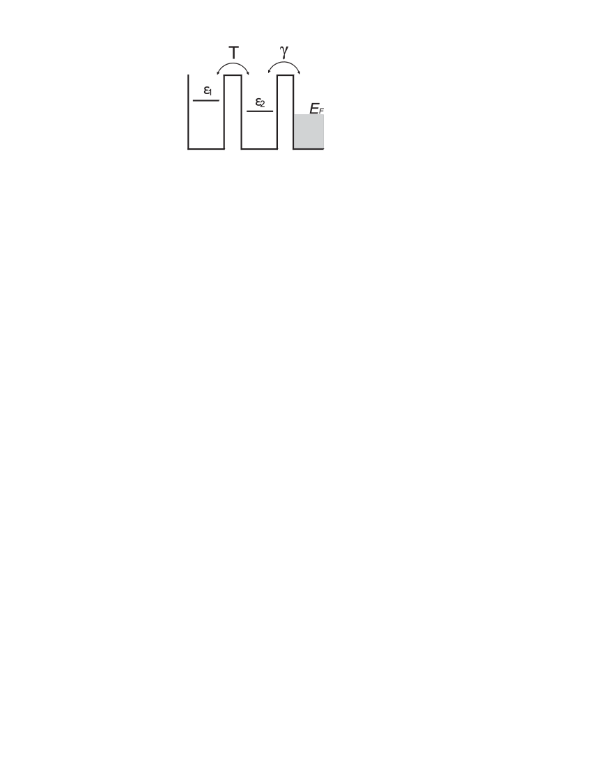
Figure 2: Schematic diagram of energy levels in the system of two coupled QDs. Second QD is also connected with continuous spectrum states.

We assume that at the initial moment all charge density in the system is localized in the first QD and has the value $n_{1}(0)$. First of all we have to calculate exact retarded Green functions of the system. In the absence of tunneling between the QDs Green functions $G_{11}^{0R}(t-t^{{}^{\prime}})$ and $G_{22}^{0R}(t-t^{{}^{\prime}})$ are determined by the expressions:

$$G_{11}^{0R}(t-t^{{}^{\prime}}) = -i\Theta(t-t^{{}^{\prime}})e^{-i\varepsilon_{1}(t-t^{{}^{\prime}})}$$

$$G_{22}^{0R}(t-t^{{}^{\prime}}) = -i\Theta(t-t^{{}^{\prime}})e^{-i\varepsilon_{2}(t-t^{{}^{\prime}})-\gamma(t-t^{{}^{\prime}})}$$ (12)

where $\gamma=\pi\nu_{k}^{0}T_{k}^{2}$ is the tunneling relaxation rate from the second QD to the continuous spectrum states.

Retarded electron Green’s function $G_{11}^{R}$ yields density of states in the first QD and can be found exactly from the integral equation:

$$G_{11}^{R}=G_{11}^{0R}+G_{11}^{0R}T^{2}G_{22}^{0R}G_{11}^{R}$$ (13)

The eigenfrequencies $E_{1,2}$ of equation (13) are determined in the following way:

$$(E-\varepsilon_{1})(E-\varepsilon_{2}+i\gamma)-T^{2}=0$$

$$E_{1,2}=\frac{1}{2}(\varepsilon_{1}+\varepsilon_{2}-i\gamma)\pm\frac{1}{2}\sqrt{(\varepsilon_{1}-\varepsilon_{2}+i\gamma)^{2}+4T^{2}}$$ (14)

Finally retarded Green’s function can be written as:

$$G_{11}^{R}(t,t^{{}^{\prime}})=-i\Theta(t-t^{{}^{\prime}})(\frac{E_{1}-\varepsilon_{2}+i\gamma}{E_{1}-E_{2}}e^{-E_{1}(t-t^{{}^{\prime}})}-$$

$$-\frac{E_{2}-\varepsilon_{2}+i\gamma}{E_{1}-E_{2}}e^{-E_{2}(t-t^{{}^{\prime}})})$$ (15)

Let us now analyze time evolution of the electron density in the considered system. Electron density time evolution is governed by the Keldysh Green function $G_{11}^{<}(t,t^{{}^{\prime}})$ Keldysh :

$$G_{11}^{<}(t,t)=in_{1}(t)$$ (16)

Equation for Green function $G_{11}^{<}$ has the form:

$$G_{11}^{<}(t,t^{{}^{\prime}})=G_{11}^{0<}+G_{11}^{0<}T^{2}G_{22}^{0A}G_{11}^{A}+$$

$$+G_{11}^{0R}T^{2}G_{22}^{0R}G_{11}^{<}+G_{11}^{0R}T^{2}G_{22}^{0<}G_{11}^{A}$$

Acting with operator $G_{11}^{0R-1}$ it can be re-written as:

$$G_{11}^{0R-1}G_{11}^{<}(t,t^{{}^{\prime}})=(i\frac{\partial}{\partial t}-\varepsilon_{1})G_{11}^{<}(t,t^{{}^{\prime}})=$$

$$=T^{2}\int_{0}^{\infty}dt_{1}G_{22}^{0R}(t,t_{1})G_{11}^{<}(t_{1},t^{{}^{\prime}})+$$

$$+T^{2}\int_{0}^{\infty}dt_{1}G_{22}^{0<}(t,t_{1})G_{11}^{A}(t_{1},t^{{}^{\prime}})$$ (18)

or in a compact form:

$$(G_{11}^{0R-1}-T^{2}G_{22}^{0R})G_{11}^{<}=T^{2}G_{22}^{0<}G_{11}^{A}$$ (19)

Green function $G_{11}^{<}(t,t)$ is determined by the sum of homogeneous and inhomogeneous solutions. Inhomogeneous solution of the equation can be written in the following way:

$$G_{11}^{<}(t,t^{{}^{\prime}})=T^{2}\int_{0}^{t}dt_{1}\int_{0}^{t^{{}^{\prime}}}dt_{2}G_{11}^{R}(t-t_{1})\cdot$$

$$\cdot G_{22}^{0<}(t_{1}-t_{2})G_{11}^{A}(t_{2}-t^{{}^{\prime}})$$

Green function $G_{22}^{0<}$ can be found from equations (3) and (4) substituting index $2$ instead of $1$.

$$G_{22}^{0<}(t,t^{{}^{\prime}})=in_{2}(0)\cdot e^{-\gamma(t+t^{{}^{\prime}})}\cdot e^{-i\varepsilon_{2}(t-t^{{}^{\prime}})}+$$

$$+\frac{i}{\pi}\int d\omega\cdot f(\omega)\cdot$$

$$\cdot\frac{\gamma}{(\omega-\varepsilon_{2})^{2}+\gamma^{2}}\cdot[e^{-i\omega(t-t^{{}^{\prime}})}+e^{-i\varepsilon_{2}(t-t^{{}^{\prime}})-\gamma(t+t^{{}^{\prime}})}$$

$$-e^{-i\varepsilon_{2}t-\gamma t+i\omega t^{{}^{\prime}}}-e^{i\varepsilon_{2}t^{{}^{\prime}}-\gamma t^{{}^{\prime}}-i\omega t}]$$ (21)

Green function $G_{22}^{0<}$ contains part with exponential decay, oscillating term and part which determine stationary solution. In what follows we’ll consider the situation with $\frac{\varepsilon_{i}-\varepsilon_{F}}{\gamma}>>1$ for simplicity. It means that stationary occupation number in the second QD in the absence of coupling between QDs is of the order of $\frac{\gamma}{\varepsilon_{2}-\varepsilon_{F}}<<1$. So we can omit corresponding terms in expression (21) for function $G_{22}^{0<}$.

As we consider initial charge to be localized in the first QD, Green function $G_{22}^{0<}(0,0)\simeq 0$ and Green function $G_{11}^{<}(t,t^{{}^{\prime}})$ can be determined by the solution of homogeneous equation. Homogeneous solution of the differential equation has the form:

$$G_{11}^{<}(t,t^{{}^{\prime}})=f_{1}(t^{{}^{\prime}})e^{-iE_{1}t}+f_{2}(t^{{}^{\prime}})e^{-iE_{2}t}$$ (22)

Since $G^{<}(t,t^{{}^{\prime}})$ satisfies the symmetry relation:

$$(G_{11}^{<}(t,t^{{}^{\prime}}))^{*}=-G_{11}^{<}(t^{{}^{\prime}},t),$$ (23)

it has the following form:

$$G_{11}^{<}(t^{{}^{\prime}},t)=iAe^{-iE_{1}t+iE_{1}^{*}t^{{}^{\prime}}}+iBe^{-iE_{1}t+iE_{2}^{*}t^{{}^{\prime}}}+$$

$$+iB^{*}e^{-iE_{2}t+iE_{1}^{*}t^{{}^{\prime}}}+iCe^{-iE_{2}t+iE_{2}^{*}t^{{}^{\prime}}}$$ (24)

As far as solution has to satisfy homogeneous integro-differential equation (19)(without right hand part), after substituting expression (22) to equation (19) one can find the following relation:

$$\frac{f_{1}(t^{{}^{\prime}})}{f_{2}(t^{{}^{\prime}})}=-\frac{\varepsilon_{2}-E_{1}-i\gamma}{\varepsilon_{2}-E_{2}-i\gamma}$$ (25)

Using the initial condition:

$$G_{11}^{<}(0,0)=in_{1}^{0}$$ (26)

Time dependence of the filling number $n_{1}(t)$ in the first QD can be obtained:

$$n_{1}(t) = n_{1}^{0}\cdot(A^{{}^{\prime}}e^{-i(E_{1}-E_{1}^{*})t}+2Re(B^{{}^{\prime}}e^{-i(E_{1}-E_{2}^{*})t})+$$ (27)

$$+ C^{{}^{\prime}}e^{-i(E_{2}-E_{2}^{*})t})$$

where coefficients $A^{\prime}$, $B^{\prime}$ and $C^{\prime}$ are equal to:

$$A^{{}^{\prime}} = \frac{|E_{2}-\varepsilon_{1}|^{2}}{|E_{2}-E_{1}|^{2}};C^{{}^{\prime}}=\frac{|E_{1}-\varepsilon_{1}|^{2}}{|E_{2}-E_{1}|^{2}}$$

$$B^{{}^{\prime}} = -\frac{(E_{2}-\varepsilon_{1})(E_{1}^{*}-\varepsilon_{1})}{|E_{2}-E_{1}|^{2}}$$ (28)

Electron density time evolution in the second QD is determined by the Green function $G_{22}^{<}(t,t^{{}^{\prime}})$ with initial condition $G_{22}^{<}(0,0)=0$. Green function $G_{22}^{<}(t,t^{{}^{\prime}})$ can be found from equation similar to equation (19) with the following indexes changing ($1\leftrightarrow 2$). Due to the initial conditions $n_{2}(0)=0$, $n_{1}(0)=n_{0}$, filling numbers in the second QD $n_{2}(t)$ are determined by the inhomogeneous part of the solution. Electron filling numbers time dependence in the second QD $n_{2}(t)$ can be written as:

$$n_{2}(t) = (De^{-i(E_{1}-E_{1}^{*})t}+2Re(Ee^{-i(E_{1}-E_{2}^{*})t})+$$ (29)

$$+ Fe^{-i(E_{2}-E_{2}^{*})t})$$

where coefficients $D$, $E$ and $F$ are :

$$D=F=\frac{T^{2}}{|E_{2}-E_{1}|^{2}};\quad E=-\frac{T^{2}}{|E_{2}-E_{1}|^{2}}$$ (30)

Expressions (27) and (29) looks like there are three relaxation channels with different time scales. The first and the second relaxation channels are connected with relaxation rates $(|E_{1}-E_{1}^{*}|)$ and $(|E_{2}-E_{2}^{*}|)$ . One more time scale is connected with the expression $(|E_{1}-E_{2}^{*}|)$. This time scale is responsible for charge density oscillations in the both QDs, when the following ratio between $T$ and $\gamma$ is valid: $T/\gamma>1/2$.

In the resonance $\varepsilon_{1}\simeq\varepsilon_{2}$ one can find four different regimes of the system behavior:

1) Realization of the condition $2T<\gamma$ leads to the absence of oscillations in the QDs charge density time evolution. In this case the following expressions are valid:

$$E_{1}-E_{1}^{*} = -i\gamma(1-\sqrt{1-(4T^{2})/\gamma^{2}})$$

$$E_{2}-E_{2}^{*} = -i\gamma(1+\sqrt{1-(4T^{2})/\gamma^{2}})$$

$$E_{1}-E_{2}^{*} = -i\gamma$$

2) When condition $2T\ll\gamma$ is fulfilled time evolution of the electron density in the first QD can be described by the expression:

$$n_{1}(t)=n_{1}^{0}\left[\left(1+\frac{2T^{2}}{\gamma^{2}}\right)e^{-{{\bf\frac{2T^{2}}{\gamma}}}t}-\frac{2T^{2}}{\gamma^{2}}e^{\displaystyle-{{\bf\gamma}}t}\right]$$

In this case the main part of the charge decreases with the relaxation rate

$$\gamma_{res}=2T^{2}/\gamma$$ (32)

3) A special regime exists in the system when condition $2T=\gamma$ is valid. Relaxation of the charge in the QDs is non exponential:

$$n_{1}(t)=n_{1}^{0}(1+\gamma t)e^{\displaystyle-\gamma t}$$

$$n_{2}(t)=\gamma^{2}t^{2}e^{\displaystyle-\gamma t}$$ (33)

4) In the case when condition $2T>\gamma$ takes place charge density oscillations can be seen in the both QDs with the typical frequency $\Omega=\sqrt{4T^{2}-\gamma^{2}}$, for $2T\gg\gamma$:

$$n_{1}(t)=n_{1}^{0}e^{-\gamma t}\,\frac{1}{2}\,\left[1+{\rm cos}(2Tt)\right]\quad$$ (34)

Let’s now analyze non-resonance case. If we are far from the resonance, relation $|\varepsilon_{1}-\varepsilon_{2}|\gg\gamma,T$ takes place, and the filling numbers relaxation law in the first QD has the form:

$$n_{1}(t)=n_{1}^{0}\big{[}\left(1-\frac{2T^{2}}{(\varepsilon_{1}-\varepsilon_{2})^{2}}\right)e^{-{{\bf\frac{2T^{2}}{(\varepsilon_{1}-\varepsilon_{2})^{2}}\gamma}}t}+$$

$$+\frac{2T^{2}}{(\varepsilon_{1}-\varepsilon_{2})^{2}}\,{\rm cos}[(\varepsilon_{1}-\varepsilon_{2})t]\,e^{-{{\bf\gamma}}t}\big{]}$$ (35)

Relaxation rates $\gamma_{res}$ and $\gamma_{nonres}$ in the resonant and non-resonant cases are connected with each other by the relations:

$$\gamma_{res}=\frac{2T^{2}}{\gamma}\qquad\gamma_{nonres}=\gamma_{res}\frac{\gamma^{2}}{(\varepsilon_{1}-\varepsilon_{2})^{2}}$$ (36)

It is not surprising of course that $\gamma_{res}\gg\gamma_{nonres}$

Let us take into account Coulomb interaction between localized electrons in the QDs. In this case interaction Hamiltonian can be written as:

$$H_{int}=U_{2}n_{2\sigma}n_{2-\sigma}+U_{1}n_{1\sigma}n_{1-\sigma}$$ (37)

We shall use self-consistent mean field approximation. It means that in the derived expressions for the filling numbers time evolution it is necessary to substitute energy level value $\varepsilon_{i}$ ($i=1,2$) by the expression $\widetilde{\varepsilon}_{i}=\varepsilon_{i}+U\cdot<n_{i}(t)>$. Then one should solve self-consistent system of equations for $n_{i}(t)$. We shall analyze only paramagnetic case: $n_{i\sigma}=n_{i-\sigma}=n_{i}$.

Such approximation can be applied when the following relations are fulfilled:

$$|E_{1}-E_{1}^{*}|\ll min(|E_{1}|,|E_{2}|)$$

$$|E_{2}-E_{2}^{*}|\ll min(|E_{1}|,|E_{2}|)$$

$$|E_{1}-E_{2}^{*}|\ll min(|E_{1}|,|E_{2}|)$$ (38)

Inequalities (38) mean that one can uncouple rapidly oscillating Green functions ($G_{11}^{R}$ and $G_{22}^{R}$) and slowly changing functions $n_{1}(t)$ and $n_{2}(t)$. Suggested conditions are analogous to the approximations which are used in the adiabatic approach. In the mean-field approximation the main effect of Coulomb interaction deals with the detuning changing between energy levels $\varepsilon_{1}$ and $\varepsilon_{2}$. So for simplicity we shall take into account Coulomb interaction only in the second QD coupled with the continuous spectrum states. Further we’ll demonstrate that the presence of on-site Coulomb repulsion in both QDs slightly modifies the obtained results.

Let us discuss the application possibility of the mean-field approximation in the considered non-stationary case. For the stationary case when electron filling numbers are changed by variation of the applied bias or gate voltage in mixed-valence regime Anderson conditions $U/\gamma\geq 1$ and $(\varepsilon_{i}-\varepsilon_{F})/\gamma\geq 1$ are important for the validity of the mean-field approximation. We are interested in the non-stationary effects, so these conditions are not so crucial. Slow variations of energy levels due to the localized charge time evolution allows to obtain reasonable results in the self-consistent mean-field approximation even in the presence of strong Coulomb interaction. We also want to point out that initial energy levels are situated well above the Fermi level $(\varepsilon_{i}-\varepsilon_{F})/\gamma>>1$, so stationary Kondo effect can not appear. Energy level in the QD connected with continuous spectrum is nearly empty. Of course non-zero electron density appears in the second QD during localized charge relaxation. So one can try to investigate non-stationary Kondo effect and estimate the time scale of many-particle correlated state formation. The simple estimation of this time scale $\tau$ is connected with the inverse width of Kondo peak.

$$\tau^{-1}\sim\gamma_{Kondo}\sim\sqrt{(\varepsilon_{2}+U)\cdot\varepsilon_{2}}\cdot e^{-\frac{\varepsilon_{2}\cdot(\varepsilon_{2}+U)}{U\gamma}}$$ (39)

Consequently relative values of the system parameters $U/\varepsilon_{2}$, $U/\gamma$, $T/\gamma$ and $\varepsilon_{2}/\gamma$ determine it’s behaviour. Our investigations deals with the typical parameters values demonstrated below on Fig.5-Fig.6. For these values of parameters $\gamma_{Kondo}\sim 1\times 10^{-2}\gamma$, so $\tau\sim 1\times 10^{2}\cdot\tau_{0}$, where $\tau_{0}$ is the localized charge relaxation time in the second QD due to the interaction with continuous spectrum. More careful $\tau$ estimation can be based on the approach suggested in Glazman . We can consider energy level $\varepsilon_{2}$ position changing due to the effect of Coulomb interaction $U<n_{2}(t)>$ to be similar to the influence of time dependent gate voltage on the electron energies in QDs leading to the spin flip. So following the logic of Glazman et. al. Glazman one can obtain:

$$\tau^{-1}\sim(\gamma\cdot\frac{T^{2}}{\gamma^{2}}\cdot\frac{U}{\varepsilon_{2}})^{2}\cdot(\frac{\gamma}{\varepsilon_{2}})^{2}\cdot(\frac{U}{\varepsilon_{2}+U})^{2}$$ (40)

For typical values of system parameters (Fig.5-Fig.6) $\tau^{-1}\sim 10^{-2}\gamma$.

Thus characteristic time of Kondo peak formation is much larger than the localized charge relaxation time.

IV Charge relaxation in the coupled QDs in the presence of on-site Coulomb repulsion

We start by discussing the case of weak Coulomb interaction when the ratio $Un_{2}(t)/\gamma\leq\Delta\varepsilon/\gamma$ is fulfilled (Fig.5). If the initial detuning between energy levels has positive value ($\varepsilon_{1}>\varepsilon_{2}$ Fig.3a) localized charge relaxation rate in the first QD and full charge density in the second QD increase (Fig.5a,b grey line) in comparison with the case when Coulomb interaction is absent (Fig.5a,b black line). Relaxation rate increases due to the decreasing of initial detuning value $\Delta\varepsilon/\gamma$ caused by Coulomb interaction (Fig.3a, Fig.4). Fig.4 demonstrates the detuning time evolution and reveals that in the absence of Coulomb interaction energy levels detuning has constant value (Fig.4 grey dashed line). The presence of on-site Coulomb repulsion results in the smaller detuning values in the system except the initial time moment and time period when the system is quite empty and Coulomb interaction can be neglected (Fig.4 grey line).

In the opposite case of negative initial energy levels detuning ($\varepsilon_{1}<\varepsilon_{2}$ Fig.3b) even small values of Coulomb interaction results in the effective increasing of energy levels spacing (Fig.4 black line). Consequently, relaxation rate in the first QD and full charge density in the second QD decrease (Fig.5a dashed line) in comparison with the case when Coulomb interaction is absent (Fig.5b dashed line) and detuning takes on constant value.

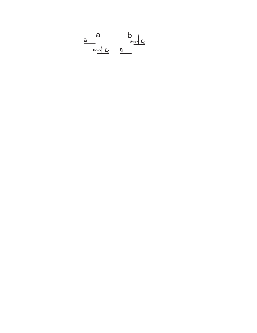
Figure 3: Schematic diagram of energy levels position for different signs of detuning in the presence of Coulomb interaction.

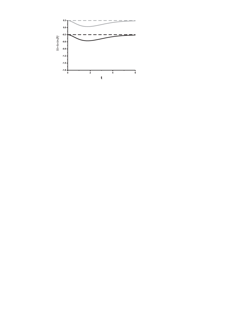
Figure 4: Energy levels detuning time evolution. $U/\gamma=0$ and positive initial detuning $(\varepsilon_{1}-\varepsilon_{2})/\gamma=(6.3-6.0)/1=0.3$-grey dashed line; $U/\gamma=0$ and negative initial detuning $(\varepsilon_{1}-\varepsilon_{2})/\gamma=(6.0-6.3)/1=-0.3$-black dashed line; $U/\gamma=3$ and positive initial detuning $(\varepsilon_{1}-\varepsilon_{2})/\gamma=(6.3-6.0)/1=0.3$-grey line; $U=3$ and negative initial detuning $(\varepsilon_{1}-\varepsilon_{2})/\gamma=(6.0-6.3)/1=-0.3$-black line.

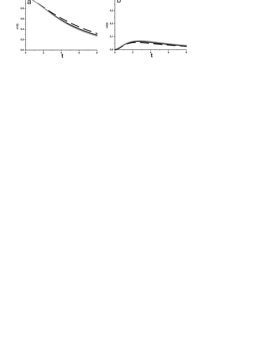
Figure 5: Filling numbers evolution in the first a). $n_{1}(t)$ and second b). $n_{2}(t)$ QDs. $U/\gamma=0$-black line both for positive $(\varepsilon_{1}-\varepsilon_{2})/\gamma=(6.3-6.0)/1=0.3$ and negative $(\varepsilon_{1}-\varepsilon_{2})/\gamma=(6.0-6.3)/1=-0.3$ detuning, $U/\gamma=3$ and $(\varepsilon_{1}-\varepsilon_{2})/\gamma=(6.3-6.0)/1=0.3$ -grey line, $U/\gamma=3$ and $(\varepsilon_{1}-\varepsilon_{2})/\gamma=(6.0-6.3)/1=-0.3$-dashed line. Parameters $T/\gamma=0.6$ and $\gamma=1.0$ are the same for all the figures.

Let us now focus on the charge relaxation processes due to the presence of strong Coulomb interaction ($Un_{2}(t)/\gamma\geq\Delta\varepsilon/\gamma$) and positive initial detuning (Fig.6). In this case filling numbers time evolution in the first QD reveals three typical time intervals with different values of the relaxation rates. The first one corresponds to the time interval $0<t<t_{02max}$, where $t_{02max}$- is an instant of time when the filling numbers in the second QD reach maximum value $n_{2max}$ (Fig.6b). Simultaneously filling numbers in the first QD demonstrate the relaxation rate changing (bend formation) (Fig.6a). The appropriate detuning behavior is presented on the Fig.7. One can find that the presence of strong on-site Coulomb repulsion results in fast compensation of initial positive detuning. Further time evolution leads to the formation of negative detuning between energy levels and it is clearly evident that the filling numbers maximum in the second QD corresponds to the maximum energy levels spacing. This time interval reveals charge relaxation with the typical rate very close to the $\gamma_{res}$. Coulomb interaction increasing in this time interval results in the weak decreasing of relaxation rate in comparison with the case when Coulomb correlations are neglected.

The next time interval $t_{02max}<t<t_{01min}$ ($t_{01min}$-is an instant of time when the filling numbers in the first QD $n_{1}(t)$ achieve minimum value $n_{1min}$) reveals localized charge relaxation with the typical rate very close to the $\gamma_{nonres}$. Filling numbers time evolution in the first and second QDs simultaneously demonstrates dip’s formation (Fig.6a,b) which corresponds to the local minimum of the effective detuning (Fig.7). This phenomenon can be explained by the influence of the following physical mechanism: charge redistribution between the QDs by means of relaxation channel with the typical relaxation rate $(|E_{1}-E_{2}^{*}|)$ (eq.27) in the presence of strong on-site Coulomb repulsion. Charge redistribution strongly governs the system behavior in the second time interval due to the presence of significant real part of the relaxation rate $(|E_{1}-E_{2}^{*}|)$ which is proportional to the value $Un_{2}(t)$ (Fig.8 grey line). In the first time interval relaxation occurs regularly because real part of the relaxation rate $(|E_{1}-E_{2}^{*}|)$ is negligible or nearly absent due to the small values of filling numbers in the second QD. Contribution from the charge redistribution mechanism becomes crucial only when filling numbers in the second QD reach maximum value. These effect self-consistently influence the charge dynamics in the proposed system by means of effective detuning changing.

The third time interval demonstrates charge relaxation with the typical rate very close to the $\gamma_{res}$. This interval exists due to the decreasing of the filling numbers amplitude in the second QD. It leads to the increasing of the relaxation rate value in comparison with the previous time interval. The presence of on-site Coulomb repulsion leads to the small detuning values in comparison with the second time interval due to the fact that the system is quite empty and Coulomb interaction can be neglected (Fig.7). Consequently charge redistribution also can be omitted. Therefore with the increasing of time the effective detuning aspire to the value without any Coulomb correlations in the system.

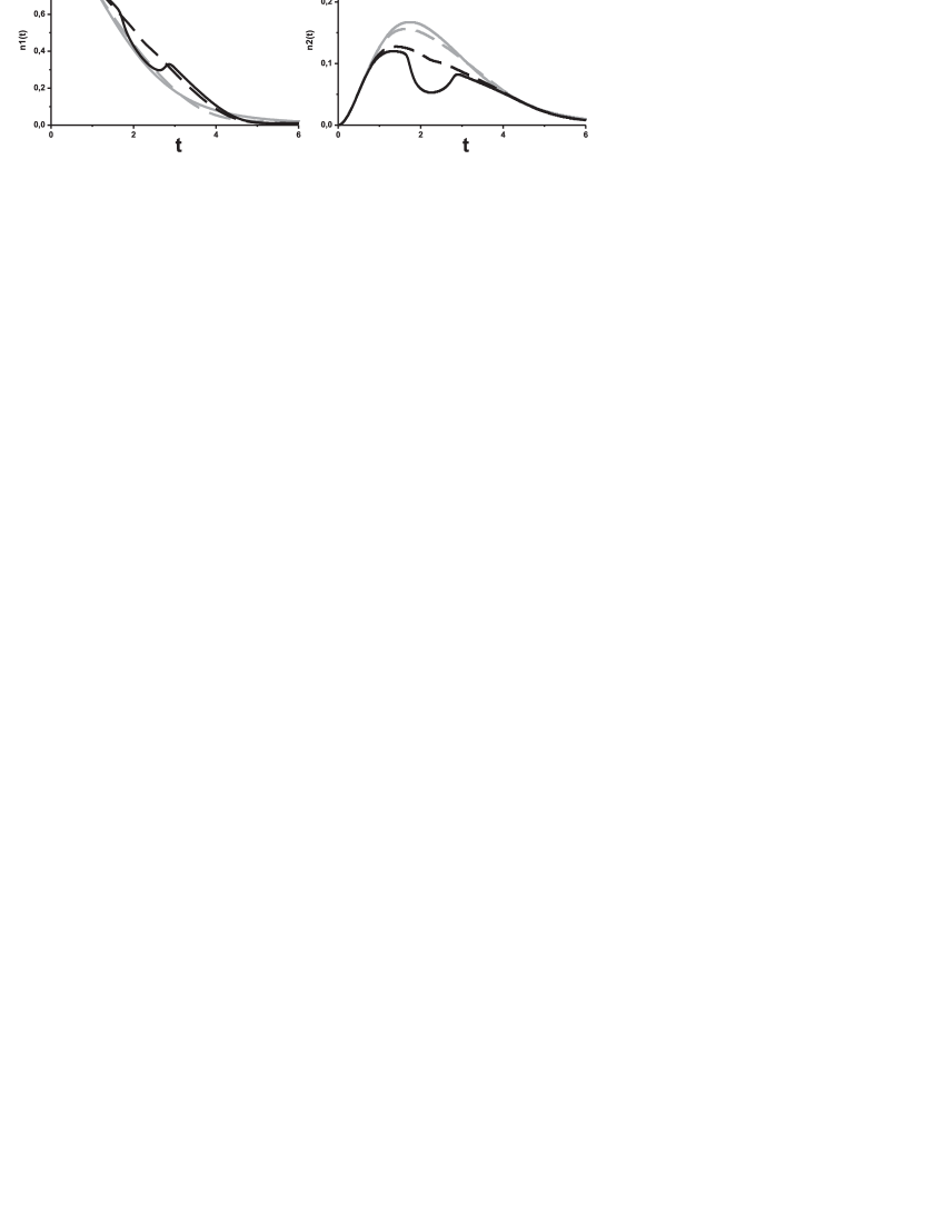
Figure 6: Filling numbers evolution in the first a). $n_{1}(t)$ and second b). $n_{2}(t)$ QDs. $U/\gamma=0$-grey line, $U/\gamma=6$-grey dashed line, $U/\gamma=12$-black dashed line, $U/\gamma=14$-black line. Parameters $(\varepsilon_{1}-\varepsilon_{2})/\gamma=(6.3-6.0)/1=0.3$, $T/\gamma=0.6$ and $\gamma=1.0$ are the same for all the figures.

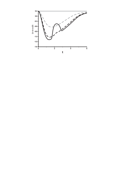
Figure 7: Energy levels detuning time evolution in the case of positive initial detuning $(\varepsilon_{1}-\varepsilon_{2})/\gamma=(6.3-6.0)/1=0.3$. $U/\gamma=0$-grey line; $U/\gamma=6$-grey dashed line; $U/\gamma=12$-black dashed line; $U/\gamma=14$-black.

Strong Coulomb interaction significantly influence on the relaxation processes. To analyze the mechanism of relaxation law modification one have to examine the relaxation exponents evolution, which determine charge relaxation rates changing in each channel of the QDs. Moreover we shall analyze time evolution of the preexponential factors which govern charge re-distribution between the relaxation channels. This analysis will be carried out for the most interesting case of positive initial detuning, when Coulomb interaction leads to the dip’s formation.

Let us start from the analysis of the exponents evolution. Their behavior is just the same for the both QDs (Fig.8). In the absence of Coulomb interaction second channel relaxation rate $E_{2}-E_{2}^{*}$ always exceeds the first channel $E_{1}-E_{1}^{*}$ relaxation rate. This ratio between relaxation rates also takes place at the initial time moment in the presence of Coulomb interaction. Coulomb interaction results in the dip and peak formation in the second and first relaxation channels accordingly (Fig.8a,b). First channel relaxation rate maximum value corresponds to the second channel relaxation rate minimum value. For the large time values evolution laws demonstrate constant values of relaxation rates for both relaxation channels equal to the values obtained without Coulomb interaction. Splitting of the peak in the first relaxation channel and dip in the second one can be seen with further increasing of Coulomb interaction. Moreover peaks in the first relaxation channel correspond to the dips in the second relaxation channel and dip in the first relaxation channel corresponds to the peak in the second relaxation channel (Fig.8c).

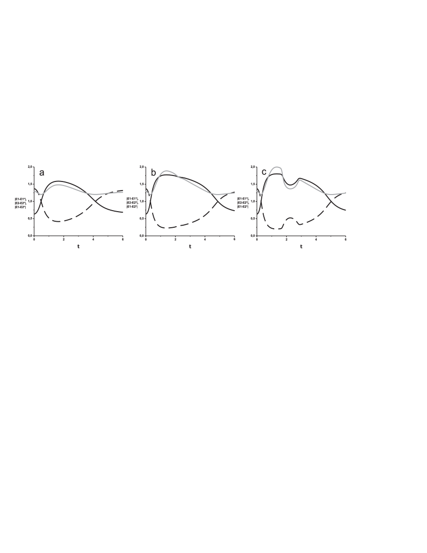
Figure 8: Each channel relaxation rates time evolution for the values of parameters $(\varepsilon_{1}-\varepsilon_{2})/\gamma=(6.3-6.0)/1=0.3$; $T/\gamma=0.6$; $\gamma=1.0$. $E_{1}-E_{1}^{*}$-black line; $E_{2}-E_{2}^{*}$-dashed black line; $E_{1}-E_{2}^{*}$-grey line; a). $U/\gamma=6$; b). $U/\gamma=12$; c). $U/\gamma=14$.

Let us now focus on the preexponential factors (relaxation channel’s amplitudes) time evolution in the presence of Coulomb interaction. In the second QD preexponential factors time evolution is determined by the same law ($D(t)$ and $F(t)$ expression 30) (Fig. 9 grey line). Time evolution of the preexponential factors in the first QD is quite different ($A(t)$ and $C(t)$ expression 28).

First relaxation channel amplitude always exceeds second relaxation channel amplitude in the first QD and both relaxation channels amplitudes in the second QD in the absence of Coulomb interaction. This ratio is also valid at the initial time moment in the case of Coulomb interaction between localized electrons.

Relaxation channel’s amplitudes time evolution in the second QD ($D(t)$ and $F(t)$ in Fig.9b) demonstrates maximum which corresponds to the minimum for the both relaxation channel’s amplitudes in the first QD for small Coulomb interaction values. With the increasing of Coulomb interaction (Fig.9b) first relaxation channel amplitude in the first QD $A(t)$ and both relaxation channel’s amplitudes in the second QD ($D(t)$ and $F(t)$) tend to zero, second relaxation channel amplitude in the first QD $C(t)$ tends to the unity. Further time evolution demonstrates that all channels amplitudes in both QDs turn to constant values equal to the values obtained without Coulomb interaction.

Increasing of the Coulomb interaction results in simultaneous peaks formation for all the relaxation channels (Fig.9c).

Comparing the obtained results which describe exponents evolution (charge relaxation rates in each channel) and evolution of the preexponential factors (time evolution of the each relaxation channel amplitude) one can easily reveal that charge redistribution between the relaxation channels in the same QD occurs. At the initial moment most part of the charge is concentrated in the first relaxation channel of the first QD and later localized charge redistributes to the second relaxation channel of the first QD. The following time increasing again demonstrates charge localization in the first relaxation channel of the first QD. Charge in the second QD is equally distributed between both relaxation channels.

Charge relaxation in the presence of Coulomb interaction in both quantum dots is determined by the charge density redistribution among different channels in the same QD and by the changing of relaxation rates of each channel. So due to Coulomb interaction the leading mechanism of non-monotonic charge relaxation in each QD is charge redistribution between the channels in a separate QD at particular range of the system parameters.

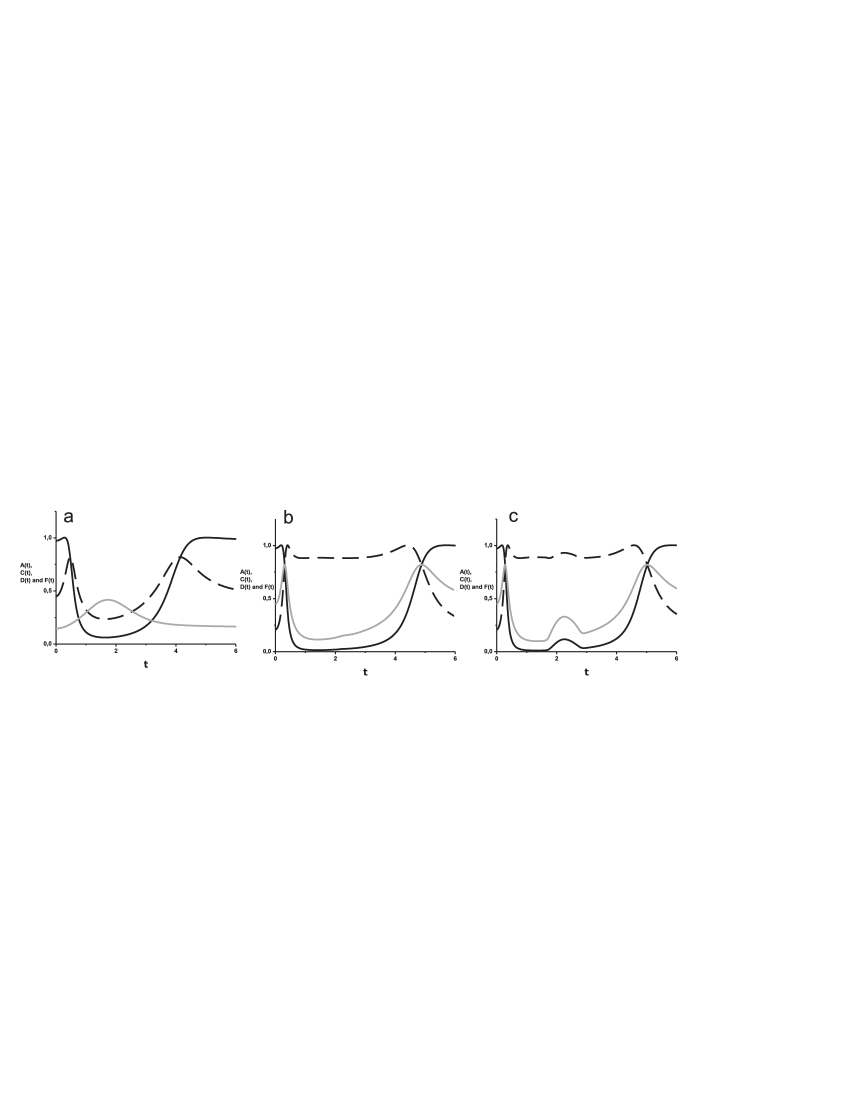
Figure 9: Each relaxation channel amplitude time evolution as a function of time for the values of parameters $(\varepsilon_{1}-\varepsilon_{2})/\gamma=(6.3-6.0)/1=0.3$; $T/\gamma=0.6$; $\gamma=1.0$. Preexponential factor for the first relaxation channel in the first QD $A(t)$-black line; preexponential factor for the second relaxation channel in the first QD $C(t)$-dashed black line; preexponential factors for the first and second relaxation channels in the second QD $D(t)$ and $F(t)$-grey line. a). $U/\gamma=6$; b). $U/\gamma=12$; c). $U/\gamma=14$.

The last point of our discussion deals with comparison between results obtained for suggested model and more natural from experimental point of view situation when Coulomb interaction is taken into account in both QDs. Fig.10 demonstrates localized charge time evolution for the both relaxation channels. Grey line corresponds to the case when Coulomb interaction exists only in the second QD and black-dashed line describes the situation when Coulomb interaction is taken into account in the both QDs. It is evident that Coulomb interaction in the both QDs results in more rapid compensation of energy levels detuning for $\Delta\varepsilon/\gamma>0$ and doesn’t lead to qualitative changes of the obtained results. So (as it was mentioned above) for simplicity it is sufficient to consider Coulomb interaction only in one QD. In any case Coulomb interaction effectively changes level spacing, which control the charge redistribution between the relaxation channels in a single QD as well as between two QDs.

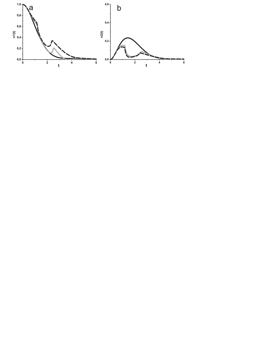
Figure 10: Filling numbers evolution in the first a). $n_{1}(t)$ and second b). $n_{2}(t)$ QDs without Coulomb interaction ($U_{1}/\gamma=0$ and $U_{2}/\gamma=0$-black line), with Coulomb interaction in the second QD ($U_{1}=0$ and $U_{2}=14$-grey line), with Coulomb interaction in both QDs ($U_{1}/\gamma=3$ and $U_{2}/\gamma=14$- black dashed line). Parameters $(\varepsilon_{1}-\varepsilon_{2})/\gamma=(6.3-6.0)/1=0.3$, $T/\gamma=0.6$ and $\gamma=1.0$ are the same for all the figures.

IV.1 Conclusion

We have analyzed time evolution of localized charge in the system of two interacting QDs both in the absence and in the presence of Coulomb interaction between localized electrons within a particular quantum dot. We have found that Coulomb interaction modifies the relaxation rates and the character of localized charge time evolution. It was shown that several time ranges with considerably different relaxation rates arise in the system of two coupled QDs. We demonstrated that the presence of Coulomb interaction leads to strong charge redistribution between different relaxation channels in each QD. So we can conclude that non-monotonic behavior of charge density is not the result of charge redistribution between the QDs but is determined by charge redistribution between the relaxation channels in a single QD.

In any real situation Coulomb interaction is present in both QDs. But for simplicity it is sufficient to consider Coulomb interaction only in one QD since the main role of Coulomb interaction is charge redistribution between the relaxation channels in a single QD as well as between QDs due to modification of the detuning between energy levels in QDs.

V Acknowledgements

We acknowledged the financial support from RFBR and Leading Scientific School grants.

References

- (1) M.A. Kastner, Rev. Mod. Phys., 4, (1992), 849.
- (2) R. Ashoori, Nature, 379, (1996), 413.
- (3) T.H. Oosterkamp, T. Fujisawa, W.G. van der Wiel et.al., Nature, 395, (1998), 873.
- (4) R.H. Blick, D. van der Weide, R.J. Haug et.al., Phys.Rev Lett., 81, (1998), 689.
- (5) C.A. Stafford, N. Wingreen, Phys. Rev. Lett., 76,(1996), 1916.
- (6) B. Hazelzet, M. Wagewijs, H. Stoof et.al., Phys.Rev. B, 63, (2001), 165313.
- (7) E. Cota, R. Aguadado, G. Platero, Phys.Rev Lett., 94, (2005), 107202.
- (8) F.R. Waugh, M.J. Berry, D.J. Mar et.al., Phys. Rev. Lett., 75, (1995), 705.
- (9) R.H. Blick, R.J. Haug, J. Weis et.al., Phys.Rev B, 53, (1996), 7899.
- (10) C.A. Stafford, S. Das Sarma, Phys. Rev. Lett., 72, (1994), 3590.
- (11) K.A. Matveev, L.I. Glazman, H.U. Baranger, Phys.Rev. B, 54, (1996), 5637.
- (12) C. Livermore, C.H. Crouch, R.M. Westervelt et.al., Science, 274, (1996), 1332.
- (13) S. J. Angus, A.J. Ferguson, A.S. Dzurak et. al., Nano Lett., 7, (2007), 2051.
- (14) K. Grove-Rasmussen, H. Jorgensen, T. Hayashi et. al., Nano Lett., 8, (2008), 1055.
- (15) S. Moriyama, D. Tsuya, E. Watanabe et. al., Nano Lett., 9, (2009), 2891.
- (16) R. Landauer, Science, 272, (1996), 1914.
- (17) D. Loss, D.P. DiVincenzo, Phys. Rev. A, 57, (1998), 120.
- (18) K.Y. Tan, K.W. Chan, M. Mottonen et. al., Nano Lett., 10, (2010), 11.
- (19) L.C.L. Hollenberg, A.D. Greentree, A.G. Fowler et.al, Phys.Rev. B, 74, (2006), 045311.
- (20) T. Hayashi, T. Fujisawa, H. Cheong et.al., Phys.Rev. Lett., 91, (2003), 226804-1.
- (21) I. Bar-Joseph, S.A. Gurvitz, Phys.Rev. B, 44, (1991), 3332.
- (22) S.A. Gurvitz, M.S. Marinov, Phys.Rev. A, 40, (1989), 2166.
- (23) S.A. Gurvitz, G. Kalbermann, Phys.Rev. Lett, 59, (1987), 262.
- (24) L.V. Keldysh Sov. Phys. JETP, 20, (1964), 1018.
- (25) P.W. Anderson, Phys.Rev., 164, (1967), 352.
- (26) A. Kaminski, Yu.N. Nazarov, L.I. Glazman, Phys.Rev. B, 62, (2000), 8154.