Approximation of the Fokker-Planck equation
of the stochastic chemostat

Abstract

We consider a stochastic model of the two-dimensional chemostat as a diffusion process for the concentration of substrate and the concentration of biomass. The model allows for the washout phenomenon: the disappearance of the biomass inside the chemostat. We establish the Fokker-Planck associated with this diffusion process, in particular we describe the boundary conditions that modelize the washout. We propose an adapted finite difference scheme for the approximation of the solution of the Fokker-Planck equation.
Keywords:chemostat, stochastic differential equation, Fokker-Planck equation, finite difference scheme

1 Introduction

Many biotechnological processes are modelized with the help of ordinary differential equations (ODE). For example, the dynamic for a single species/single substrate chemostat is classically modelized as [12]:

$$\dot{s}(t) =-k\,\mu(s(t))\,b(t)+D\,(s_{\textrm{\tiny in}}-s(t))\,,$$ (1a)

$$\dot{b}(t) =\{\mu(s(t))-D\}\,b(t)$$ (1b)

where $b(t)$ and $s(t)$ are the concentrations of biomass and substrate at time $t$ inside the chemostat. The parameters are the dilution rate $D$, the input substrate concentration $s_{\textrm{\tiny in}}$, and the stoichiometric coefficient $k$. The specific growth function $\mu(s)$ could be of the Monod (non-inhibitory) type:

$$\mu(s) =\frac{\mu_{\textrm{\tiny\rm max}}\,s}{k_{s}+s}\,,$$ (2)

where $\mu_{\textrm{\tiny\rm max}}$ is the maximum growth rate and $k_{s}$ is the half-saturation; it could also be of the Haldane (inhibitory) type:

$$\mu(s) =\frac{\bar{\mu}\,s}{k_{s}+s+s^{2}/\alpha}\,.$$ (3)

As pointed out in [2], the system (1) is simple and applicable to many situations, it can be seen as a limit model of a stochastic birth and death process in high population size asymptotic. Hence (1) can give account for the mean behavior of the underlying stochastic process but it cannot give account for its the variance. Moreover (1) fails to propose a realistic representation of the chemostat in small population scenario, that is in cases close to the washout (corresponding to the disappearance of the biomass, i.e. $b(t)=0$).

We present the stochastic model in Section 2 and derive the associated Fokker-Planck equation in Section 3. A finite difference scheme approximation is detailled in Section 4 and some numerical tests are presented in Section 5.

2 The stochastic chemostat model

Consider the stochastic process $X_{t}=(X^{1}_{t},X^{2}_{t})=(S_{t},B_{t})$ solution of:

$${{\textrm{d}}}S_{t} =\big{\{}-k\,\mu(S_{t})\,B_{t}+D\,(s_{\textrm{\tiny in}}-S_{t})\big{\}}\,{{\textrm{d}}}t+c_{1}\,\sqrt{S_{t}}\,{{\textrm{d}}}W^{1}_{t}\,,$$ (4a)

$${{\textrm{d}}}B_{t} =\{\mu(S_{t})-D\}\,B_{t}\,{{\textrm{d}}}t+c_{2}\,\sqrt{B_{t}}\,{{\textrm{d}}}W^{2}_{t}\,,$$ (4b)

where $B_{t}$ and $S_{t}$ are the concentrations of biomass and substrate at time $t$; $W_{t}^{1}$ and $W_{t}^{2}$ are independent scalar standard Brownian motions; $c_{1}>0$ and $c_{2}>0$ are the noise intensities; $W^{1}_{t}$ and $W^{2}_{t}$ are independent scalar standard Wiener processes. We suppose that $S_{0}\geq 0$ and $B_{0}\geq 0$ so that $S_{t}\geq 0$ and $B_{t}\geq 0$ for all $t\geq 0$.

The precise analysis of the behavior of the solution of (4) will be addressed in a forthcoming work [3]. Still we can describe it simply with some highlights about the classic Cox-Ingersoll-Ross model. Consider the one–dimensional SDE:

$${{\textrm{d}}}\xi_{t}=(a+b\,\xi_{t})\,{{\textrm{d}}}t+\sigma\,\sqrt{\xi_{t}}\,{{\textrm{d}}}W_{t}\,,\quad\xi_{0}=x_{0}\geq 0\,.$$ (5)

with $a\geq 0$, $b\in\mathbb{R}$, $\sigma>0$. According to [10, Prop. 6.2.4], for all $x_{0}\geq 0$, $\xi_{t}$ is a continuous process taking values in $\mathbb{R}^{+}$, and let $\tau=\inf\{t\geq 0,\,\xi_{t}=0\}$, then:

1. If $a\geq\sigma^{2}/2$, then $\tau=\infty$ $\mathbb{P}_{x}$–a.s.;

2. if $0\leq a<\sigma^{2}/2$ and $b\leq 0$ then $\tau<\infty$ $\mathbb{P}_{x}$–a.s.;

3. if $0\leq a<\sigma^{2}/2$ and $b>0$ then $\mathbb{P}_{x}(\tau<\infty)\in(0,1)$.

In the first case, $\xi_{t}$ never reaches 0. In the second case $\xi_{t}$ a.s. reaches the state 0, in the third case it may reach 0. If $a=0$ then the state 0 is absorbing.

In case of the System (4), it is clear that $B=0$ is an absorbing state for (4b), and when $B=0$, (4a) reduces to the substrate dynamics conditionally of the washout, namely:

$${{\textrm{d}}}S^{\textrm{\tiny\rm v}}_{t} =D\,(s_{\textrm{\tiny in}}-S^{\textrm{\tiny\rm v}}_{t})\,{{\textrm{d}}}t+c_{1}\,\sqrt{S^{\textrm{\tiny\rm v}}_{t}}\,{{\textrm{d}}}W^{1}_{t}$$ (6)

hence the solution of this SDE will stay on the half-line $[0,\infty)$ and:

1. if $D\,s_{\textrm{\tiny in}}\geq\frac{c_{1}^{2}}{2}$ then $S_{t}$ never reaches $0$;

2. if $D\,s_{\textrm{\tiny in}}<\frac{c_{1}^{2}}{2}$ then $S_{t}$ reaches $0$ in finite time and is reflected.

Note that, as $c_{1}$ is “small”, condition (i) is more realistic than condition (ii): indeed, with a continuous input $s_{\textrm{\tiny in}}$ , there is no reason for the substrate concentration in the chemostat to vanish.

Simulation schemes for (4) should respect the previous properties, an adequate choice is:

$$S_{t+\delta} =\big{[}S_{t}+\big{\{}-k\,\mu(S_{t})\,B_{t}+D\,(s_{\textrm{\tiny in}}-S_{t})\big{\}}\,\delta+c_{1}\,\sqrt{S_{t}}\,\sqrt{\delta}\,w^{1}_{t}\big{]}_{+}\,,$$ (7a)

$$B_{t+\delta} =\big{[}B_{t}+\{\mu(S_{t})-D\}\,B_{t}\,\delta+c_{2}\,\sqrt{B_{t}}\,\sqrt{\delta}\,w^{2}_{t}\big{]}_{+}\,,$$ (7b)

where $\{w^{1}_{i\delta}\}_{i\in\mathbb{N}}$ and $\{w^{2}_{i\delta}\}_{i\in\mathbb{N}}$ are i.i.d. $N(0,1)$ random variables, also independent from $X_{0}$. Note that $B_{t}=0$ is absorbing for (7b).

Notations 2.1

Let $x=(x_{1},x_{2})=(s,b)\in\mathbb{R}^{2}_{+}=[0,\infty)^{2}$ and

$$f_{1}(x)=f_{1}(s,b) \stackrel{{\scriptstyle{\textrm{\rm\tiny def}}}}{{=}}-k\,\mu(s)\,b+D\,(s_{\textrm{\tiny in}}-s)\,, \sigma_{1}(x)=\sigma_{1}(s,b)=\sigma_{1}(s) \stackrel{{\scriptstyle{\textrm{\rm\tiny def}}}}{{=}}c_{1}\,\sqrt{s}\,,$$

$$f_{2}(x)=f_{2}(s,b) \stackrel{{\scriptstyle{\textrm{\rm\tiny def}}}}{{=}}[\mu(s)-D]\,b\,, \sigma_{2}(x)=\sigma_{2}(s,b)=\sigma_{2}(b) \stackrel{{\scriptstyle{\textrm{\rm\tiny def}}}}{{=}}c_{2}\,\sqrt{b}\,,$$

so that (4) reads:

$${{\textrm{d}}}X_{t} =f(X_{t})\,{{\textrm{d}}}t+\sigma(X_{t})\,{{\textrm{d}}}W_{t}$$

with $f(x)=\left(\begin{smallmatrix}f_{1}(x)\\ f_{2}(x)\end{smallmatrix}\right)$, $\sigma(x)=\left(\begin{smallmatrix}\sigma_{1}(x)&0\\ 0&\sigma_{2}(x)\end{smallmatrix}\right)$ and $W_{t}=\left(\begin{smallmatrix}W^{1}_{t}\\ W^{2}_{t}\end{smallmatrix}\right)$.

Let $\partial{\mathbb{R}^{2}_{+}}=\Gamma_{1}\cup\Gamma_{2}$ with $\Gamma_{1}=\{(s,b)\in[0,\infty)^{2}\,;\,b=0\}$ and $\Gamma_{2}=\{(s,b)\in[0,\infty)^{2}\,;\,s=0\}$.

3 The Fokker-Planck equation

Let $\pi_{t}({{\textrm{d}}}x)=\pi_{t}({{\textrm{d}}}s,{{\textrm{d}}}b)$ be the distribution law of of $X_{t}=(S_{t},B_{t})$:

$$\pi_{t}(A,B)=\mathbb{P}(S_{t}\in A\,,\ B_{t}\in B)$$

for all Borel sets $A,B$ of $[0,\infty)$. According to [11], $\pi_{t}({{\textrm{d}}}x)$ of $X_{t}$ can be decomposed as:

$$\pi_{t}({{\textrm{d}}}x)=\pi_{t}({{\textrm{d}}}s\times{{\textrm{d}}}b)=\delta_{0}({{\textrm{d}}}b)\,q_{t}(s)\,{{\textrm{d}}}s+p_{t}(s,b)\,{{\textrm{d}}}s\,{{\textrm{d}}}b$$ (8)

indeed the diffusion process “lives” in ${\mathbb{R}^{2}_{+}}$ but never reaches $\Gamma_{2}$ so the distribution law features only a “regular” component $p_{t}(s,b)$ that only charges ${\mathring{\mathbb{R}}^{2}_{+}}$ and a “degenerate” component $q_{t}(s)$ that only charges $\Gamma_{1}$.

As $\pi_{t}$ is a probability distribution we get the normalization property:

$$\int_{0}^{\infty}q_{t}(s)\,{{\textrm{d}}}s+\int_{0}^{\infty}\int_{0}^{\infty}p_{t}(s,b)\,{{\textrm{d}}}s\,{{\textrm{d}}}b=1\,.$$

and the washout probability at time $t$ is:

$$\mathbb{P}(B_{t}=0)=\int_{0}^{\infty}q_{t}(s)\,{{\textrm{d}}}s=1-\int_{0}^{\infty}\int_{0}^{\infty}p_{t}(s,b)\,{{\textrm{d}}}s\,{{\textrm{d}}}b\,.$$

The Fokker-Planck equation in a weak form is:

$$\frac{{{\textrm{d}}}}{{{\textrm{d}}}t}\iint_{\mathbb{R}^{2}_{+}}\pi_{t}({{\textrm{d}}}s,{{\textrm{d}}}b)\,\phi(s,b) =\iint_{\mathbb{R}^{2}_{+}}\pi_{t}({{\textrm{d}}}s,{{\textrm{d}}}b)\,{\mathcal{L}}\phi(s,b)$$ (9)

for all test functions $\phi$, where ${\mathcal{L}}$ is the infinitesimal generator defined by:

$${\mathcal{L}}\phi(x) ={\mathcal{L}}\phi(s,b)$$

$$\stackrel{{\scriptstyle{\textrm{\rm\tiny def}}}}{{=}}\sum_{i=1}^{2}f_{i}(x)\,\phi^{\prime}_{x_{i}}(x)+\frac{1}{2}\,\sum_{i=1}^{2}\sigma^{2}_{i}(x)\,\phi^{\prime\prime}_{x_{i}^{2}}(x)$$

$$=\textstyle f_{1}(s,b)\,\phi^{\prime}_{s}(s,b)+f_{2}(s,b)\,\phi^{\prime}_{b}(s,b)+\frac{c_{1}^{2}}{2}\,s\,\phi^{\prime\prime}_{s^{2}}(s,b)+\frac{c_{2}^{2}}{2}\,b\,\phi^{\prime\prime}_{b^{2}}(s,b)\,.$$ (10)

Using the decomposition (8), the Fokker-Planck equation (9) reads:

$$\frac{{{\textrm{d}}}}{{{\textrm{d}}}t}\Big{\{}\int_{0}^{\infty}q_{t}(s)\,\phi(s,0)\,{{\textrm{d}}}s+\iint_{\mathbb{R}^{2}_{+}}p_{t}(s,b)\,\phi(s,b)\,{{\textrm{d}}}s\,{{\textrm{d}}}b\Big{\}}=$$

$$\qquad\qquad\qquad\qquad=\int_{0}^{\infty}q_{t}(s)\,{\mathcal{L}}\phi(s,0)\,{{\textrm{d}}}s+\iint_{\mathbb{R}^{2}_{+}}p_{t}(s,b)\,{\mathcal{L}}\phi(s,b)\,{{\textrm{d}}}s\,{{\textrm{d}}}b$$ (11)

Lemma 3.1

For all functions $\phi\in H^{2}_{\Gamma_{2}}({\mathbb{R}^{2}_{+}})$ (i.e. $\phi\in H^{1}({\mathbb{R}^{2}_{+}})$ and $\phi|_{\Gamma_{2}}=0$) and $t\geq 0$

$$\langle p_{t},{\mathcal{L}}\phi\rangle =\int_{\mathbb{R}^{2}_{+}}{\mathcal{L}}^{*}p_{t}(x)\,\phi(x)\,{{\textrm{d}}}x+\frac{c_{2}^{2}}{2}\,\int_{0}^{\infty}p_{t}(s,0)\,\phi(s,0)\,{{\textrm{d}}}s$$

where ${\mathcal{L}}^{*}$ is the adjoint operator:

$${\mathcal{L}}^{*}\psi(x)\stackrel{{\scriptstyle{\textrm{\rm\tiny def}}}}{{=}}\textstyle-[\psi(x)\,f_{1}(x)]^{\prime}_{s}-[\psi(x)\,f_{2}(x)]^{\prime}_{b}+\frac{c_{1}^{2}}{2}\,[\psi(x)\,s]^{\prime\prime}_{s^{2}}+\frac{c_{2}^{2}}{2}\,[\psi(x)\,b]^{\prime\prime}_{b^{2}}\,.$$

Proof

By definition of ${\mathcal{L}}$:

$$\langle p_{t},{\mathcal{L}}\phi\rangle=\textstyle\int_{{\mathbb{R}^{2}_{+}}}p_{t}(x)\,{\mathcal{L}}\phi(x)\,{{\textrm{d}}}x =\textstyle\int_{\mathbb{R}^{2}_{+}}p_{t}(x)\,f_{1}(x)\,\phi^{\prime}_{s}(x)\,{{\textrm{d}}}x+\int_{\mathbb{R}^{2}_{+}}p_{t}(x)\,f_{2}(x)\,\phi^{\prime}_{b}(x)\,{{\textrm{d}}}x$$

$$\qquad\textstyle+\frac{c_{1}^{2}}{2}\,\int_{\mathbb{R}^{2}_{+}}p_{t}(x)\,s\,\phi^{\prime\prime}_{s^{2}}(x)\,{{\textrm{d}}}x+\frac{c_{2}^{2}}{2}\,\int_{\mathbb{R}^{2}_{+}}p_{t}(x)\,b\,\phi^{\prime\prime}_{b^{2}}(x)\,{{\textrm{d}}}x$$

we consider separately these four last terms.

From Green’s formula [1]: $\int_{{\mathbb{R}^{2}_{+}}}u^{\prime}_{x_{i}}\,v\,{{\textrm{d}}}x=-\int_{{\mathbb{R}^{2}_{+}}}u\,v^{\prime}_{x_{i}}\,{{\textrm{d}}}x+\int_{\partial{\mathbb{R}^{2}_{+}}}u\,v\,n_{i}\,{{\textrm{d}}}\SS_{x}$ where $n_{i}$ is the $i$th component of the outward unit normal $n$, i.e. $n_{1}(x)=0$ on $\Gamma_{1}$ and $-1$ on $\Gamma_{2}$ and $n_{2}(x)=-1$ on $\Gamma_{1}$ and $0$ on $\Gamma_{2}$. So we get:

$$\textstyle\int_{\mathbb{R}^{2}_{+}}p_{t}(x)\,f_{1}(x)\,\phi^{\prime}_{s}(x)\,{{\textrm{d}}}x =\textstyle-\int_{\mathbb{R}^{2}_{+}}[p_{t}(x)\,f_{1}(x)]^{\prime}_{s}\,\phi(x)\,{{\textrm{d}}}x+\int_{\partial{\mathbb{R}^{2}_{+}}}p_{t}(x)\,f_{1}(x)\,\phi(x)\,n_{1}(x)\,{{\textrm{d}}}\SS_{x}$$

$$\textstyle=-\int_{\mathbb{R}^{2}_{+}}[p_{t}(x)\,f_{1}(x)]^{\prime}_{s}\,\phi(x)\,{{\textrm{d}}}x-\int_{\Gamma_{2}}p_{t}(x)\,f_{1}(x)\,\phi(x)\,{{\textrm{d}}}\SS_{x}$$

$$\textstyle=-\int_{\mathbb{R}^{2}_{+}}[p_{t}(x)\,f_{1}(x)]^{\prime}_{s}\,\phi(x)\,{{\textrm{d}}}x\,. \phi=0 \Gamma_{2}$$ (as on )

For the second term:

$$\textstyle\int_{\mathbb{R}^{2}_{+}}p_{t}(x)\,f_{2}(x)\,\phi^{\prime}_{b}(x)\,{{\textrm{d}}}x =\textstyle-\int_{\mathbb{R}^{2}_{+}}[p_{t}(x)\,f_{2}(x)]^{\prime}_{b}\,\phi(x)\,{{\textrm{d}}}x+\int_{\partial{\mathbb{R}^{2}_{+}}}p_{t}(x)\,f_{2}(x)\,\phi(x)\,n_{2}(x)\,{{\textrm{d}}}\SS_{x}$$

$$=\textstyle-\int_{\mathbb{R}^{2}_{+}}[p_{t}(x)\,f_{2}(x)]^{\prime}_{b}\,\phi(x)\,{{\textrm{d}}}x-\int_{\Gamma_{1}}p_{t}(x)\,f_{2}(x)\,\phi(x)\,{{\textrm{d}}}\SS_{x}$$

$$=\textstyle-\int_{\mathbb{R}^{2}_{+}}[p_{t}(x)\,f_{2}(x)]^{\prime}_{b}\,\phi(x)\,{{\textrm{d}}}x\,. f_{2}=0 \Gamma_{1}$$ (as on )

For the third term:

$$\textstyle\int_{\mathbb{R}^{2}_{+}}p_{t}(x)\,s\,\phi^{\prime\prime}_{s^{2}}(x)\,{{\textrm{d}}}x =\textstyle-\int_{\mathbb{R}^{2}_{+}}[p_{t}(x)\,s]^{\prime}_{s}\,\phi^{\prime}_{s}(x)\,{{\textrm{d}}}x+\int_{\partial{\mathbb{R}^{2}_{+}}}p_{t}(x)\,s\,\phi^{\prime}_{s}(x)\,n_{1}(x)\,{{\textrm{d}}}\SS_{x}$$

$$=\textstyle-\int_{\mathbb{R}^{2}_{+}}[p_{t}(x)\,s]^{\prime}_{s}\,\phi^{\prime}_{s}(x)\,{{\textrm{d}}}x-\int_{\Gamma_{2}}p_{t}(x)\,s\,\phi^{\prime}_{s}(x)\,{{\textrm{d}}}\SS_{x}$$

$$=\textstyle-\int_{\mathbb{R}^{2}_{+}}[p_{t}(x)\,s]^{\prime}_{s}\,\phi^{\prime}_{s}(x)\,{{\textrm{d}}}x s=0 \Gamma_{2}$$ (as on )

$$=\textstyle\int_{\mathbb{R}^{2}_{+}}[p_{t}(x)\,s]^{\prime\prime}_{s^{2}}\,\phi(x)\,{{\textrm{d}}}x-\int_{\partial{\mathbb{R}^{2}_{+}}}[p_{t}(x)\,s]^{\prime}_{s}\,\phi(x)\,n_{1}(x)\,{{\textrm{d}}}\SS_{x}$$

$$=\textstyle\int_{\mathbb{R}^{2}_{+}}[p_{t}(x)\,s]^{\prime\prime}_{s^{2}}\,\phi(x)\,{{\textrm{d}}}x+\int_{\Gamma_{2}}[p_{t}(x)\,s]^{\prime}_{s}\,\phi(x)\,{{\textrm{d}}}\SS_{x}$$

$$=\textstyle\int_{\mathbb{R}^{2}_{+}}[p_{t}(x)\,s]^{\prime\prime}_{s^{2}}\,\phi(x)\,{{\textrm{d}}}x\,. \phi=0 \Gamma_{2}$$ (as on )

For the fourth term:

$$\textstyle\int_{\mathbb{R}^{2}_{+}}p_{t}(x)\,b\,\phi^{\prime\prime}_{b^{2}}(x)\,{{\textrm{d}}}x =\textstyle-\int_{\mathbb{R}^{2}_{+}}[p_{t}(x)\,b]^{\prime}_{b}\,\phi^{\prime}_{b}(x)\,{{\textrm{d}}}x+\int_{\partial{\mathbb{R}^{2}_{+}}}p_{t}(x)\,b\,\phi^{\prime}_{b}(x)\,n_{2}(x)\,{{\textrm{d}}}\SS_{x}$$

$$=\textstyle-\int_{\mathbb{R}^{2}_{+}}[p_{t}(x)\,b]^{\prime}_{b}\,\phi^{\prime}_{b}(x)\,{{\textrm{d}}}x-\int_{\Gamma_{1}}p_{t}(x)\,b\,\phi^{\prime}_{b}(x)\,{{\textrm{d}}}\SS_{x}$$

$$=\textstyle-\int_{\mathbb{R}^{2}_{+}}[p_{t}(x)\,b]^{\prime}_{b}\,\phi^{\prime}_{b}(x)\,{{\textrm{d}}}x b=0 \Gamma_{1}$$ (as on )

$$=\textstyle\int_{\mathbb{R}^{2}_{+}}[p_{t}(x)\,b]^{\prime\prime}_{b^{2}}\,\phi(x)\,{{\textrm{d}}}x-\int_{\partial{\mathbb{R}^{2}_{+}}}[p_{t}(x)\,b]^{\prime}_{b}\,\phi(x)\,n_{2}(x)\,{{\textrm{d}}}\SS_{x}$$

$$=\textstyle\int_{\mathbb{R}^{2}_{+}}[p_{t}(x)\,b]^{\prime\prime}_{b^{2}}\,\phi(x)\,{{\textrm{d}}}x+\int_{\Gamma_{1}}[p_{t}(x)\,b]^{\prime}_{b}\,\phi(x)\,\,{{\textrm{d}}}\SS_{x}\,.$$

Summing up these identities leads to:

$$\langle p_{t},{\mathcal{L}}\phi\rangle=\textstyle\langle{\mathcal{L}}^{*}\,p_{t},\phi\rangle+\frac{c_{2}^{2}}{2}\,\int_{\Gamma_{1}}[p_{t}(x)\,b]^{\prime}_{b}\,\phi(x)\,\,{{\textrm{d}}}\SS_{x}$$

finally

$$\textstyle\int_{\Gamma_{1}}[p_{t}(x)\,b]^{\prime}_{b}\,\phi(x)\,\,{{\textrm{d}}}\SS_{x} =\textstyle\int_{\Gamma_{1}}\big{\{}[p_{t}(x)]^{\prime}_{b}\,b+p_{t}(x)\big{\}}\,\phi(x)\,\,{{\textrm{d}}}\SS_{x}$$

$$=\textstyle\int_{\Gamma_{1}}p_{t}(x)\,\phi(x)\,\,{{\textrm{d}}}\SS_{x}$$

$$=\textstyle\int_{0}^{\infty}p_{t}(s,0)\,\phi(s,0)\,\,{{\textrm{d}}}s$$

proves the lemma. $\Box$

According to Lemma 3.1, (11) becomes:

$$\frac{{{\textrm{d}}}}{{{\textrm{d}}}t}\Big{\{}\int_{0}^{\infty}q_{t}(s)\,\phi(s,0)\,{{\textrm{d}}}s+\iint_{\mathbb{R}^{2}_{+}}p_{t}(s,b)\,\phi(s,b)\,{{\textrm{d}}}s\,{{\textrm{d}}}b\Big{\}}=$$

$$\qquad\qquad=\int_{0}^{\infty}q_{t}(s)\,{\mathcal{L}}\phi(s,0)\,{{\textrm{d}}}s+\iint_{\mathbb{R}^{2}_{+}}{\mathcal{L}}^{*}p_{t}(s,b)\,\phi(s,b)\,{{\textrm{d}}}s\,{{\textrm{d}}}b$$

$$\qquad\qquad\qquad\qquad+\frac{c_{2}^{2}}{2}\,\int_{0}^{\infty}p_{t}(s,0)\,\phi(s,0)\,{{\textrm{d}}}s$$ (12)

Let $\phi(s,b)=\varphi(s)\,\psi(b)$ with $\psi(0)=1$, $\psi(b)=0$ for $b>\varepsilon$ and $\psi^{\prime}(0)=\psi^{\prime\prime}(0)=0$, after letting $\varepsilon\to 0$, the previous equation leads to:

$$\frac{{{\textrm{d}}}}{{{\textrm{d}}}t}\int_{0}^{\infty}q_{t}(s)\,\varphi(s)\,{{\textrm{d}}}s=\int_{0}^{\infty}q_{t}(s)\,{\mathcal{G}}\varphi(s)\,{{\textrm{d}}}s+\frac{c_{2}^{2}}{2}\,\int_{0}^{\infty}p_{t}(s,0)\,\varphi(s)\,{{\textrm{d}}}s$$ (13)

where

$${\mathcal{G}}\varphi(s)=\textstyle D\,(s_{\textrm{\tiny in}}-s)\,\varphi^{\prime}(s)+\frac{c^{2}_{2}}{2}\,s\,\varphi^{\prime\prime}(s)$$ (14)

is the infinitesimal generator of the diffusion $S_{t}$ in washout mode, i.e. of the SDE (6). As (13) is valid for all test functions $\varphi$, we get the following equation for $q_{t}(s)$:

$$\frac{\partial}{\partial t}q_{t}(s) ={\mathcal{G}}^{*}q_{t}(s)+\frac{c_{2}^{2}}{2}\,p_{t}(s,0)\,, \forall t\geq 0\,,\ s\in[0,\infty)$$ (15a)

the equation for $$p_{t}(s,v)$$ is

$$\frac{\partial}{\partial t}p_{t}(s,v) ={\mathcal{L}}^{*}p_{t}(s,v)\,, \forall t\geq 0\,,\ (s,v)\in[0,\infty)^{2}$$ (15b)

The initial condition for (15a) and (15b) are:

$$q_{t}(s) =\rho_{\textrm{\tiny v}}(s)\,, p_{t}(s,v) =\rho(s,b)\,.$$ (15c)

where $\rho_{\textrm{\tiny v}}(s)\,{{\textrm{d}}}s\,\delta_{0}({{\textrm{d}}}b)+\rho(s,b)\,{{\textrm{d}}}s\,{{\textrm{d}}}b$ is the distribution law of $X_{0}=(S_{0},B_{0})$.

The operators are:

$${\mathcal{G}}^{*}\varphi(s) =\textstyle-D\,\big{[}(s_{\textrm{\tiny in}}-s)\,\varphi(s)\big{]}^{\prime}+\frac{c^{2}_{2}}{2}\,\big{[}s\,\varphi(s)\big{]}^{\prime\prime}\,,$$ (16)

$${\mathcal{L}}^{*}\phi(s,v) =\textstyle-\big{[}f_{1}(s,b)\,\phi(s,b)\big{]}^{\prime}_{s}-\big{[}f_{2}(s,b)\,\phi(s,b)\big{]}^{\prime}_{b}$$

$$\qquad\qquad\qquad\qquad\textstyle+\frac{c_{1}^{2}}{2}\,\big{[}s\,\phi(s,b)]^{\prime\prime}_{s^{2}}+\frac{c_{2}^{2}}{2}\,\big{[}b\,\phi(s,b)]^{\prime\prime}_{b^{2}}$$ (17)

Finally, the Fokker-Planck equation is a system of PDE’s: (15b) for $p_{t}(s,v)$ and (15a) for $q_{t}(s)$, the first one is autonomous, and its solution appears as an input for the second PDE.

4 Approximation

Many finite difference schemes and finite element schemes are adapted to space discretization of the system (15). Here we use the specific finite difference scheme proposed in [8]. This classical scheme presents nice numerical properties and it also can be interpreted as an approximation of the solution of (4) by a pure jump Markov process on a finite discretization grid, the resulting system in discrete-space and continuous-time is the exact Fokker-Planck equation (forward Kolmogorov equation) associated with this pure jump process. The infinitesimal generator ${\mathcal{L}}$ of the SDE (4) is given by (10), this operator fully characterizes the distribution law of the process $X_{t}=(S_{t},B_{t})$, indeed the set of equations (15) is totally determined by the operator ${\mathcal{L}}$ as ${\mathcal{G}}$ is only the restriction of ${\mathcal{L}}$ to $\Gamma_{2}$.

The finite difference scheme is detailed in A, it leads to the following approximation of the infinitesimal generator:

$${\mathcal{L}}\phi(x)\simeq{\mathcal{L}}_{h}\phi(x)=\sum_{y\in G_{h}}{\mathcal{L}}_{h}(x,y)\,\phi(y)$$

for $x\in G_{h}$ where:

$$G_{h} \stackrel{{\scriptstyle{\textrm{\rm\tiny def}}}}{{=}}\{x=(k_{1}\,h_{1},k_{2}\,h_{2})\,;\,k_{i}=0,\dots,N_{i},\,i=1,2\}\,,$$

$$\mathring{G}_{h} \stackrel{{\scriptstyle{\textrm{\rm\tiny def}}}}{{=}}\{x=(k_{1}\,h_{1},k_{2}\,h_{2})\,;\,k_{i}=1,\dots,N_{i}-1,\,i=1,2\}\,,$$

$$G^{1}_{h} \stackrel{{\scriptstyle{\textrm{\rm\tiny def}}}}{{=}}\{x=(k_{1}\,h_{1},0)\,;\,k_{1}=0,\dots,N_{1}\}\,,$$

are the grid version of ${\mathbb{R}^{2}_{+}}$, $\mathring{{\mathbb{R}^{2}_{+}}}$ and $\Gamma_{1}$ respectively, see Figure 1.

Figure 1: Discretized domain $G_{h}$.

For the interior points $x\in\mathring{G}_{h}$ the finite difference scheme is:

$$\left\{\begin{array}[]{rll}{\mathcal{L}}_{h}(x,x)&=-\frac{|f_{1}(x)|}{h_{1}}-\frac{|f_{2}(x)|}{h_{2}}-\frac{\sigma^{2}_{1}(x)}{h_{1}^{2}}-\frac{\sigma^{2}_{2}(x)}{h_{2}^{2}}\,,\\ {\mathcal{L}}_{h}(x,x\pm h_{i}\,e_{i})&=\frac{f_{i}^{\pm}(x)}{h_{i}}+\frac{\sigma^{2}_{i}(x)}{2\,h_{i}^{2}}\,,\quad i=1,2\,,\\[6.99997pt] {\mathcal{L}}_{h}(x,y)&=0\qquad\textrm{otherwise.}\end{array}\right.$$

For the boundary points $x\in G_{h}\setminus\mathring{G}_{h}$ the finite difference schemes are detailed in B. They correspond to the Figure 1: for $s=s_{\textrm{\tiny\rm max}}$ or $b=b_{\textrm{\tiny\rm max}}$, we must impose reflecting conditions, for for $s=0$ or $b=0$, the boundary conditions are natural, they derive from the value of the coefficients. Indeed, when $b=0$, then $f_{2}=\sigma_{2}=0$ and the jump process stays on the boundary “$b=0$” (it cannot jump to $b=h_{2}$ or to $b=-h_{2}$). When $s=0$, then $f_{1}=D\,s_{\textrm{\tiny in}}$ and $\sigma_{1}=0$, so the jump process can only jump to $s=h_{1}$.

We obtain a matrix ${\mathcal{L}}_{h}=[{\mathcal{L}}_{h}(x,y)]_{x,y\in G_{h}}$ which is the infinitesimal generator of a pure jump Markov process $(X^{h}_{t})_{t\geq 0}$ in continuous time and discrete state space $G_{h}$. Starting from a point $x$ of the grid, the process $X^{h}_{t}$ stays there during a time exponentially distributed with parameter $-{\mathcal{L}}_{h}(x,x)$ then it jumps to a point $y$ with probability ${\mathcal{L}}_{h}(x,y)/(-{\mathcal{L}}_{h}(x,x))$ for all $y\in{\mathcal{G}}_{h}$, and ${\mathcal{L}}_{h}$ is a ${\mathcal{Q}}$-matrix as $\sum_{y\in{\mathcal{G}}_{h}}{\mathcal{L}}_{h}(x,y)=0$. Then the following Kolmogorov forward equation:

$$\frac{\partial}{\partial t}p^{h}_{t}(x) ={\mathcal{L}}_{h}^{*}\,p^{h}_{t}(x)$$ (18)

gives the evolution of the distribution law $p^{h}_{t}$ of $X^{h}_{t}$, $p^{h}_{t}(x)=\mathbb{P}(X^{h}_{t}=x)$, $x\in G_{h}$.

It is important to note that this approach gives an approximation of the coupled system of PDEs (15): $(p^{h}_{t}(x))_{x\in G_{h}\setminus G^{1}_{h}}$ is an approximation of $(p_{t}(s,b))_{(s,b)\in(0,\infty)^{2}}$ and $(p^{h}_{t}(x))_{x\in G^{1}_{h}}$ is an approximation of $(q_{t}(s))_{s\in(0,\infty)}$.

For the time-discretization we use the implicit Euler scheme approximation:

$$\frac{p^{h}_{t+\delta}(x)-p^{h}_{t}(x)}{\delta}={\mathcal{L}}_{h}^{*}\,p^{h}_{t+\delta}(x)$$

that is:

$$(I-\delta\,{\mathcal{L}}^{*}_{h})\,p_{t+\delta}(x)=p_{t}(x)\,.$$

5 Numerical results

5.1 Comparison

Many works [7] propose the following structure for the diffusion coefficients:

$${{\textrm{d}}}S_{t} =\big{\{}-k\,\mu(S_{t})\,B_{t}+D\,(s_{\textrm{\tiny in}}-S_{t})\big{\}}\,{{\textrm{d}}}t+c_{1}\,S_{t}\,{{\textrm{d}}}W^{1}_{t}\,,$$ (19a)

$${{\textrm{d}}}B_{t} =\big{\{}\mu(S_{t})\,B_{t}-D\,B_{t}\big{\}}\,{{\textrm{d}}}t+c_{2}\,B_{t}\,{{\textrm{d}}}W^{2}_{t}\,.$$ (19b)

It is slightly different from (4). In large population size, these two models are rather equivalent; they differ drastically in the washout regime.

In this test we use the Monod growth rate function (2) and the parameters: $k=10$, $s_{\textrm{\tiny in}}=1.3$ (mg/l), $D=0.4$ (1/h), $\mu_{\textrm{\tiny\rm max}}=3$ (1/h) , $k_{s}=6$ (mg/l). The initial law is $(S_{0},B_{0})\sim{\mathcal{N}}(0.45,10^{-5})\otimes{\mathcal{N}}(0.01,10^{-5})$. The discretization parameters are $s_{\textrm{\tiny\rm max}}=2$, $b_{\textrm{\tiny\rm max}}=0.06$, $\delta=0.1$, $N_{1}=N_{2}=70$. In Figure 2, we see that with small noise intensities the simulation of the two models are very similar; with higher small noise intensities, the simulations are very different. This is due to the fact that the behavior of the two diffusion processes near the boundary “$b=0$” are different: with the model (4) the washout regime is attainable which is not the case with the model (19). In Figure 3 we compare the evolution of the washout probability $t\to\mathbb{P}(B_{t}=0)$ for both models, we clearly see that the model (19) does not give account for this probability.

$t=1$
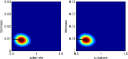
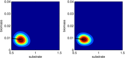
$t=5$
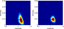
$t=10$
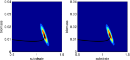
$t=15$
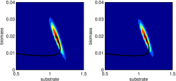
$t=20$
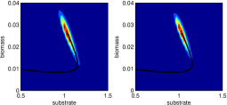
	case 1.a                  case 2.a	case 1.b                  case 2.b

Figure 2: In cases “1” the diffusion coefficients are $\sigma_{1}(s)=c_{1}\,\sqrt{s}$ and $\sigma_{2}(b)=c_{2}\,\sqrt{b}$; in cases “2” the diffusion coefficients are $\sigma_{1}(s)=c_{1}\,s$ and $\sigma_{2}(b)=c_{2}\,b$. In cases “a” $c_{1}=c_{2}=0.005$; in cases “b” $c_{1}=c_{2}=0.02$. For small noise intensities (cases “a”), cases “1” and “2” behave rather similarly. For higher noise intensities (cases “b”), as the law $\pi_{t}$ of $(S_{t},B_{t})$ is closer to the absorbing “washout” boundary $\{(s,b)\in\mathbb{R}^{2}_{+};b=0\}$, cases “1” and “2” behave rather similarly. See Figure 3 for the evaluation of the washout probability.

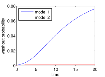
Figure 3: Washout probability — Following Figure 2: we compute $t\to\mathbb{P}(B_{t}=0)$ for the case “1” (model 1: $\sigma_{1}(s)=c_{1}\,\sqrt{s}$, $\sigma_{2}(b)=c_{2}\,\sqrt{b}$) and for case “2” (model 2: $\sigma_{1}(s)=c_{1}\,s$, $\sigma_{2}(b)=c_{2}\,b$).

5.2 Simulation with the Haldane growth rate function

In this test we use the Haldane growth rate function (3) and the parameters: $k=2$, $s_{\textrm{\tiny in}}=2.4$ (mg/l), $D=0.1$ (1/h), $\bar{\mu}=5$ (1/h) , $k_{s}=10$ (mg/l), $\alpha=0.03$: $c_{1}=c_{2}=0.01$. The initial law is $(S_{0},B_{0})\sim{\mathcal{N}}(1.5,10^{-5})\otimes{\mathcal{N}}(0.68,10^{-5})$. The discretization parameters are $s_{\textrm{\tiny\rm max}}=3$, $b_{\textrm{\tiny\rm max}}=2.5$, $\delta=0.25$, $N_{1}=N_{2}=300$.

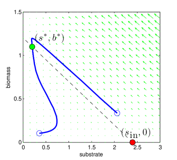
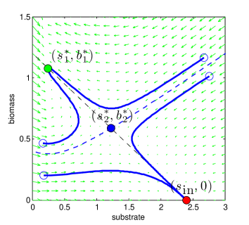
Figure 4: Phase portraits for the system (1) for the Monod growth function (left) and the Haldane growth function. Left (Monod case): there are two equilibrium states: the washout equilibrium (red dot) is unattractive, the equilibrium point $(s^{*},b^{*})$ with $s^{*}=k_{s}\,D/(\mu_{\textrm{\tiny\rm max}}-D)$ (solution of $\mu(s)=D$) and $b^{*}=(s_{\textrm{\tiny in}}-s^{*})/k$ is attractive. We suppose that $\mu_{\textrm{\tiny\rm max}}>D$. The dashed line is $b=(s_{\textrm{\tiny in}}-s)/k$, in blue two trajectories (blue circles: initial positions). Right (Haldane case): the washout is still an equilibrium point but now it is attractive, there are two other equilibrium points given as solutions of $\mu(s)=D$ (we suppose that it admits two separate solutions), $(s^{*}_{1},b^{*}_{1})$ is attractive (corresponding to the smallest value of $s$), $(s^{*}_{2},b^{*}_{2})$ is unattractive. The black dashed curve separates the two basins of attraction; in blue four trajectories (blue circles: initial positions).

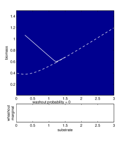
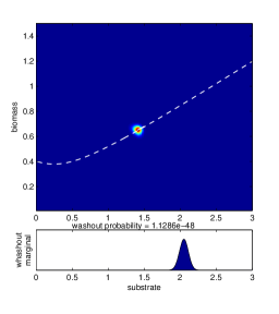
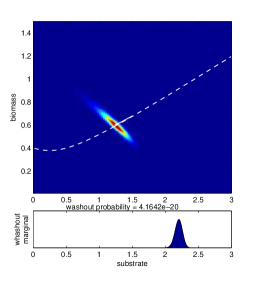
$t=0$	$t=4$	$t=24$
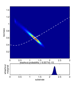
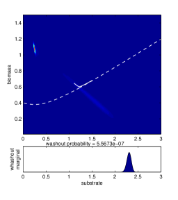
$t=32$	$t=44$	$t=52$
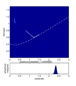
$t=68$	$t=72$	$t=80$

Figure 5: Evolution of the distribution law of $X_{t}$: for each time $t$, the density $p_{t}(s,b)$ together with the washout density $q_{t}(s)$; the dashed curve separates the two basins of attraction. The mean of $X_{0}$ is on this curve. See comments in the text.

In Figure 5 we plot the time evolution of the distribution law of $X_{t}$: for each time $t$, we represent (the approximation of) $(p_{t}(s,b);(s,b)\in(0,s_{\textrm{\tiny\rm max}})\times(0,b_{\textrm{\tiny\rm max}}))$ together with (the approximation of) $(q_{t}(s);s\in(0,s_{\textrm{\tiny\rm max}}))$. In this test the mean of $X_{0}$ is on this curve that separates the two basins of attraction (dashed white line): hence part of the mass will be attracted by $(s^{*}_{1},b^{*}_{1})$ and the other part will be attracted by the washout $(s_{\textrm{\tiny in}},0)$ (see Figure 4).

For $t=0$ we plot all the trajectory $(x(t))_{t\in[0;80]}$ (white line). At the beginning the distribution law starts to “stretch” between the two attractors ($t=24$). At $t=32$, part of the mass is already on the point $(s^{*}_{1},b^{*}_{1})$. Note that at this instant $p_{t}(s,b)$ is bimodal and $x(t)$ is a good approximation of $\mathbb{E}(X_{t})$, but it is a poor statistics for $X_{t}$. At the final time $t=80$, the deterministic trajectory $x(t)$ reaches the equilibrium point $(s^{*}_{1},b^{*}_{1})$ and $13\%$ of the mass has been trapped by the washout absorbing boundary and some mass is still in the washout basin and will be trapped by the boundary “$b=0$”.

Appendix A General finite difference scheme for $n$-dimensional diffusion processes

Let $X_{t}$ be the following diffusion process:

$${{\textrm{d}}}X_{t} =b(X_{t})\,{{\textrm{d}}}t+\sigma(X_{t})\,{{\textrm{d}}}W_{t}$$

where $X_{t}$ takes values in $\mathbb{R}^{n}$, $b:\,\mathbb{R}^{n}\mapsto\mathbb{R}^{n}$, $\sigma:\,\mathbb{R}^{n}\mapsto\mathbb{R}^{n\times m}$, and $W_{t}$ is a standard Brownian motion with values in $\mathbb{R}^{m}$. Let $a=\sigma\,\sigma^{*}:\,\mathbb{R}^{n}\mapsto\mathbb{R}^{n\times n}$. The coefficients are supposed to be locally Lipschitz and at most of linear growth.

The probability density function $p(t,x)$ of $X_{t}$ is solution of the following Fokker-Planck equation:

$$\frac{\partial}{\partial t}\,p(t,x) ={\mathcal{L}}^{*}p(t,x)$$ (20)

where ${\mathcal{L}}$ is the infinitesimal generator defined by:

$${\mathcal{L}}\phi(x) \stackrel{{\scriptstyle{\textrm{\rm\tiny def}}}}{{=}}\sum_{i=1}^{n}f_{i}(x)\,\phi^{\prime}_{x_{i}}(x)+\frac{1}{2}\,\sum_{i,j=1}^{n}a_{ij}(x)\,\phi^{\prime\prime}_{x_{i}x_{j}}(x)\,.$$

We consider finite difference schemes based on the following stencil (for the components $(x_{i},x_{j})$):

We use the following up-wind scheme [8]:

$$f_{i}(x)\,\phi^{\prime}_{x_{i}}(x) \simeq\begin{cases}f_{i}(x)\,\frac{\phi(x+h_{i}\,e_{i})-\phi(x)}{h_{i}}\,,&\textrm{ if }f_{i}(x)\geq 0\,,\\ f_{i}(x)\,\frac{\phi(x)-\phi(x-h_{i}\,e_{i})}{h_{i}}\,,&\textrm{ if }f_{i}(x)<0\,,\end{cases}$$

$$a_{ii}(x)\,\phi^{\prime\prime}_{x_{i}^{2}}(x) \simeq\textstyle a_{ii}(x)\,\frac{\phi(x+h_{i}\,e_{i})-2\,\phi(x)+\phi(x-h_{i}\,e_{i})}{h_{i}^{2}}\,,$$

$$a_{ij}(x)\,\phi^{\prime\prime}_{x_{i}x_{j}}(x) \simeq\begin{cases}\textstyle a_{ij}(x)\,\frac{1}{2\,h_{i}}\Big{[}\frac{\phi(x+h_{i}\,e_{i}+h_{j}\,e_{j})-\phi(x+h_{i}\,e_{i})}{h_{j}}-\frac{\phi(x+h_{j}\,e_{j})-\phi(x)}{h_{j}}\\ \qquad\qquad\qquad\textstyle+\frac{\phi(x)-\phi(x-h_{j}\,e_{j})}{h_{j}}-\frac{\phi(x-h_{i}\,e_{i})-\phi(x-h_{i}\,e_{i}-h_{j}\,e_{j})}{h_{j}}\Big{]}\,,\\ \qquad\qquad\qquad\qquad\qquad\qquad\qquad\qquad\qquad\textrm{ if }a_{ij}(x)\geq 0\,,\\[10.00002pt] \textstyle a_{ij}(x)\,\frac{1}{2\,h_{i}}\Big{[}\frac{\phi(x+h_{i}\,e_{i})-\phi(x+h_{i}\,e_{i}-h_{j}\,e_{j})}{h_{j}}-\frac{\phi(x)-\phi(x-h_{j}\,e_{j})}{h_{j}}\\ \qquad\qquad\qquad\textstyle+\frac{\phi(x+h_{j}\,e_{j})-\phi(x)}{h_{j}}-\frac{\phi(x-h_{i}\,e_{i}+h_{j}\,e_{j})-\phi(x-h_{i}\,e_{i})}{h_{j}}\Big{]}\,,\\ \qquad\qquad\qquad\qquad\qquad\qquad\qquad\qquad\qquad\textrm{ if }a_{ij}(x)<0\,,\end{cases}$$

for $i,j=1,\dots,n$, $i\neq j$. The last non-diagonal second order schemes correspond to the following diagrams:

With notation $f^{+}(x)=\max(f(x),0)$ and $f^{-}(x)=\max(-f(x),0)$, we get the following approximation:

$${\mathcal{L}}_{h}\phi(x)=\textstyle\sum_{i}f_{i}(x)\,\phi^{\prime}_{x_{i}}(x)+\frac{1}{2}\,\sum_{i,j}a_{i,j}(x)\,\phi^{\prime\prime}_{x_{i}x_{j}}(x)$$

$$\quad=\textstyle\sum_{i}\{f_{i}^{+}(x)-f_{i}^{-}(x)\}\,\phi^{\prime}_{x_{i}}(x)+\frac{1}{2}\,\sum_{i}a_{ii}(x)\,\phi^{\prime\prime}_{x_{i}^{2}}(x)+\frac{1}{2}\,\sum_{i,j;i\neq j}\{a_{ij}^{+}(x)-a_{ij}^{-}(x)\}\,\phi^{\prime\prime}_{x_{i}x_{j}}(x)$$

$$\quad\simeq\sum_{i}\Big{\{}\textstyle\frac{f_{i}^{+}(x)}{h_{i}}\,[\phi(x+h_{i}\,e_{i})-\phi(x)]-\frac{f_{i}^{-}(x)}{h_{i}}\,[\phi(x)-\phi(x-h_{i}\,e_{i})]\Big{\}}$$

$$\qquad\qquad+\sum_{i}\textstyle\frac{a_{ii}(x)}{2\,h_{i}^{2}}\,[\phi(x+h_{i}\,e_{i})-2\,\phi(x)+\phi(x-h_{i}\,e_{i})]$$

$$\qquad\qquad+\frac{1}{2}\,\sum_{i,j;i\neq j}\textstyle\Big{\{}\frac{a_{ij}^{+}(x)}{2\,h_{i}\,h_{j}}\,\Big{(}[\phi(x+h_{i}\,e_{i}+h_{j}\,e_{j})-\phi(x+h_{i}\,e_{i})]-[\phi(x+h_{j}\,e_{j})-\phi(x)]$$

$$\qquad\qquad\qquad\qquad\qquad\qquad\textstyle+[\phi(x)-\phi(x-h_{j}\,e_{j})]-[\phi(x-h_{i}\,e_{i})-\phi(x-h_{i}\,e_{i}-h_{j}\,e_{j})]\Big{)}$$

$$\textstyle\qquad\qquad\qquad-\frac{a_{ij}^{-}(x)}{2\,h_{i}\,h_{j}}\Big{(}[\phi(x+h_{i}\,e_{i})-\phi(x+h_{i}\,e_{i}-h_{j}\,e_{j})]-[\phi(x)-\phi(x-h_{j}\,e_{j})]$$

$$\qquad\qquad\qquad\qquad\qquad\qquad\textstyle+[\phi(x+h_{j}\,e_{j})-\phi(x)]-[\phi(x-h_{i}\,e_{i}+h_{j}\,e_{j})-\phi(x-h_{i}\,e_{i})]\Big{)}\Big{\}}$$

$$=\phi(x)\;\textstyle\Big{\{}-\sum_{i}\frac{|f_{i}(x)|}{h_{i}}-\sum_{i}\frac{a_{ii}(x)}{h_{i}^{2}}+\sum_{i,j;i\neq j}\frac{|a_{ij}(x)|}{2\,h_{i}\,h_{j}}\Big{\}}$$

$$\qquad+\textstyle\sum_{i}\phi(x+h_{i}\,e_{i})\;\textstyle\Big{\{}\frac{f_{i}^{+}(x)}{h_{i}}+\frac{a_{ii}(x)}{2\,h_{i}^{2}}-\sum_{j;j\neq i}\frac{|a_{ij}(x)|}{4\,h_{i}\,h_{j}}\Big{\}}+\sum_{j}\textstyle\sum_{i;i\neq j}\phi(x+h_{j}\,e_{j})\;\frac{|a_{ij}(x)|}{4\,h_{i}\,h_{j}}$$

$$\qquad+\textstyle\sum_{i}\phi(x-h_{i}\,e_{i})\;\textstyle\Big{\{}\frac{f_{i}^{-}(x)}{h_{i}}+\frac{a_{ii}(x)}{2\,h_{i}^{2}}-\sum_{j;j\neq i}\frac{|a_{ij}(x)|}{4\,h_{i}\,h_{j}}\Big{\}}+\sum_{j}\textstyle\sum_{i;i\neq j}\phi(x-h_{j}\,e_{j})\;\frac{|a_{ij}(x)|}{4\,h_{i}\,h_{j}}$$

$$\qquad+\textstyle\sum_{i,j;i\neq j}\textstyle\Big{\{}\frac{a_{ij}^{+}(x)}{2\,h_{i}\,h_{j}}\,[\phi(x+h_{i}\,e_{i}+h_{j}\,e_{j})+\phi(x-h_{i}\,e_{i}-h_{j}\,e_{j})]$$

$$\textstyle\qquad\qquad\qquad\qquad\qquad+\frac{a_{ij}^{-}(x)}{2\,h_{i}\,h_{j}}[\phi(x+h_{i}\,e_{i}-h_{j}\,e_{j})+\phi(x-h_{i}\,e_{i}+h_{j}\,e_{j})]\Big{\}}$$

the symmetry $a_{ij}=a_{ji}$ leads to

$${\mathcal{L}}_{h}\phi(x) =\textstyle\phi(x)\;\textstyle\Big{\{}-\sum_{i}\frac{|f_{i}(x)|}{h_{i}}-\sum_{i}\frac{a_{ii}(x)}{h_{i}^{2}}+\sum_{i,j;i\neq j}\frac{|a_{ij}(x)|}{2\,h_{i}\,h_{j}}\Big{\}}$$

$$\qquad+\textstyle\sum_{i}\phi(x+h_{i}\,e_{i})\;\textstyle\Big{\{}\frac{f_{i}^{+}(x)}{h_{i}}+\frac{a_{ii}(x)}{2\,h_{i}^{2}}-\sum_{j;j\neq i}\frac{|a_{ij}(x)|}{2\,h_{i}\,h_{j}}\Big{\}}$$

$$\qquad+\textstyle\sum_{i}\phi(x-h_{i}\,e_{i})\;\textstyle\Big{\{}\frac{f_{i}^{-}(x)}{h_{i}}+\frac{a_{ii}(x)}{2\,h_{i}^{2}}-\sum_{j;j\neq i}\frac{|a_{ij}(x)|}{2\,h_{i}\,h_{j}}\Big{\}}$$

$$\qquad+\textstyle\sum_{i,j;i\neq j}\textstyle\Big{\{}\frac{a_{ij}^{+}(x)}{2\,h_{i}\,h_{j}}\,[\phi(x+h_{i}\,e_{i}+h_{j}\,e_{j})+\phi(x-h_{i}\,e_{i}-h_{j}\,e_{j})]$$

$$\textstyle\qquad\qquad\qquad\qquad\qquad+\frac{a_{ij}^{-}(x)}{2\,h_{i}\,h_{j}}[\phi(x+h_{i}\,e_{i}-h_{j}\,e_{j})+\phi(x-h_{i}\,e_{i}+h_{j}\,e_{j})]\Big{\}}$$

We get the following approximation of the infinitesimal generator:

$${\mathcal{L}}\phi(x)\simeq{\mathcal{L}}_{h}\phi(x)=\sum_{y\in G_{h}}{\mathcal{L}}_{h}(x,y)\,\phi(y)$$

for $x\in G_{h}$ where $G_{h}=\{x=(k_{1}\,h_{1},\dots,k_{n}\,h_{n})\,;\,k_{i}=0,\dots,N_{i},\,i=1,\dots,n\}$ and

$$\left\{\begin{array}[]{rll}{\mathcal{L}}_{h}(x,x)&=-\sum_{i=1}^{n}\frac{|f_{i}(x)|}{h_{i}}-\sum_{i=1}^{n}\Big{\{}\frac{a_{ii}(x)}{h_{i}^{2}}-\sum_{j\neq i}\frac{|a_{ij}(x)|}{2\,h_{i}\,h_{j}}\Big{\}}\,,\\ {\mathcal{L}}_{h}(x,x\pm h_{i}\,e_{i})&=\frac{f_{i}^{\pm}(x)}{h_{i}}+\frac{a_{ii}(x)}{2\,h_{i}^{2}}-\sum_{j;j\neq i}\frac{|a_{ij}(x)|}{2\,h_{i}\,h_{j}}\,,\\ {\mathcal{L}}_{h}(x,x+h_{i}\,e_{i}+h_{j}\,e_{j})&={\mathcal{L}}_{h}(x,x-h_{i}\,e_{i}-h_{j}\,e_{j})=\frac{a_{ij}^{+}(x)}{2\,h_{i}\,h_{j}}\qquad\textrm{ for }i\neq j\,,\\ {\mathcal{L}}_{h}(x,x+h_{i}\,e_{i}-h_{j}\,e_{j})&={\mathcal{L}}_{h}(x,x-h_{i}\,e_{i}+h_{j}\,e_{j})=\frac{a_{ij}^{-}(x)}{2\,h_{i}\,h_{j}}\qquad\textrm{ for }i\neq j\,,\\[6.99997pt] {\mathcal{L}}_{h}(x,y)&=0\qquad\textrm{otherwise.}\end{array}\right.$$

Appendix B Boundary conditions for the finite difference approximation

For the boundary points $G_{h}\setminus\mathring{G}_{h}$ of the grid, we use the following schemes:

• For $x\in\{(s,b)\in G_{h}\,;\,s=0,b\in(0,b_{\textrm{\tiny\rm max}})\}$

  $$\left\{\begin{array}[]{rll}{\mathcal{L}}_{h}(x,x)&=-\frac{|f_{1}(x)|}{h_{1}}-\frac{|f_{2}(x)|}{h_{2}}-\frac{\sigma^{2}_{1}(x)}{h_{1}^{2}}-\frac{\sigma^{2}_{2}(x)}{h_{2}^{2}}\,,\\ {\mathcal{L}}_{h}(x,x+h_{1}\,e_{1})&=\frac{f_{1}^{+}(x)}{h_{1}}+\frac{\sigma^{2}_{1}(x)}{2\,h_{1}^{2}}\,,\\ {\mathcal{L}}_{h}(x,x-h_{1}\,e_{1})&=\frac{f_{1}^{-}(x)}{h_{1}}+\frac{\sigma^{2}_{1}(x)}{2\,h_{1}^{2}}=0\textrm{ because }f_{1}(0,b)=D\,s_{\textrm{\tiny in}}\,,\ \sigma_{1}(0,b)=0\,,\\ {\mathcal{L}}_{h}(x,x\pm h_{2}\,e_{2})&=\frac{f_{2}^{\pm}(x)}{h_{2}}+\frac{\sigma^{2}_{2}(x)}{2\,h_{2}^{2}}\,,\textrm{ note that }f_{2}(0,b)=-D\,b<0\,,\\[6.99997pt] {\mathcal{L}}_{h}(x,y)&=0\qquad\textrm{otherwise.}\end{array}\right.$$

• For $x\in\{(s,b)\in G_{h}\,;\,s=s_{\textrm{\tiny\rm max}},b\in(0,b_{\textrm{\tiny\rm max}})\}$

  $$\left\{\begin{array}[]{rll}{\mathcal{L}}_{h}(x,x)&=-\frac{|f_{1}(x)|}{h_{1}}-\frac{|f_{2}(x)|}{h_{2}}-\frac{\sigma^{2}_{1}(x)}{h_{1}^{2}}-\frac{\sigma^{2}_{2}(x)}{h_{2}^{2}}\,,\\ {\mathcal{L}}_{h}(x,x+h_{1}\,e_{1})&=0\textrm{ (set artificially to $0$)}\,,\\ {\mathcal{L}}_{h}(x,x-h_{1}\,e_{1})&=\frac{|f_{1}(x)|}{h_{1}}+\frac{\sigma^{2}_{1}(x)}{h_{1}^{2}}\,,\\ {\mathcal{L}}_{h}(x,x\pm h_{2}\,e_{2})&=\frac{f_{2}^{\pm}(x)}{h_{2}}+\frac{\sigma^{2}_{2}(x)}{2\,h_{2}^{2}}\,,\\[6.99997pt] {\mathcal{L}}_{h}(x,y)&=0\qquad\textrm{otherwise.}\end{array}\right.$$

• For $x\in\{(s,b)\in G_{h}\,;\,s\in(0,s_{\textrm{\tiny\rm max}}),b=0\}$

  $$\left\{\begin{array}[]{rll}{\mathcal{L}}_{h}(x,x)&=-\frac{|f_{1}(x)|}{h_{1}}-\frac{\sigma^{2}_{1}(x)}{h_{1}^{2}}\,,\\ {\mathcal{L}}_{h}(x,x\pm h_{1}\,e_{1})&=\frac{f_{1}^{\pm}(x)}{h_{1}}+\frac{\sigma^{2}_{1}(x)}{2\,h_{1}^{2}}\,,\\ {\mathcal{L}}_{h}(x,x\pm h_{2}\,e_{2})&=\frac{f_{2}^{\pm}(x)}{h_{2}}+\frac{\sigma^{2}_{2}(x)}{2\,h_{2}^{2}}=0\textrm{ because $f_{2}(s,0)=\sigma_{2}(s,0)=0$}\,,\\[6.99997pt] {\mathcal{L}}_{h}(x,y)&=0\qquad\textrm{otherwise.}\end{array}\right.$$

• For $x\in\{(s,b)\in G_{h}\,;\,s\in(0,s_{\textrm{\tiny\rm max}}),b=b_{\textrm{\tiny\rm max}}\}$

  $$\left\{\begin{array}[]{rll}{\mathcal{L}}_{h}(x,x)&=-\frac{|f_{1}(x)|}{h_{1}}-\frac{|f_{2}(x)|}{h_{2}}-\frac{\sigma^{2}_{1}(x)}{h_{1}^{2}}-\frac{\sigma^{2}_{2}(x)}{h_{2}^{2}}\,,\\ {\mathcal{L}}_{h}(x,x\pm h_{1}\,e_{1})&=\frac{f_{1}^{\pm}(x)}{h_{1}}+\frac{\sigma^{2}_{1}(x)}{2\,h_{1}^{2}}\,,\\ {\mathcal{L}}_{h}(x,x+h_{2}\,e_{2})&=0\textrm{ (set artificially to $0$)}\,,\\ {\mathcal{L}}_{h}(x,x-h_{2}\,e_{2})&=\frac{|f_{2}(x)|}{h_{2}}+\frac{\sigma^{2}_{2}(x)}{h_{2}^{2}}\,,\\[6.99997pt] {\mathcal{L}}_{h}(x,y)&=0\qquad\textrm{otherwise.}\end{array}\right.$$

• For $x=(0,0)$

  $$\left\{\begin{array}[]{rll}{\mathcal{L}}_{h}(x,x)&=-\frac{|f_{1}(x)|}{h_{1}}\,,\\ {\mathcal{L}}_{h}(x,x+h_{1}\,e_{1})&=\frac{f_{1}^{+}(x)}{h_{1}}\,,\\ {\mathcal{L}}_{h}(x,x-h_{1}\,e_{1})&=0\textrm{ because }f_{1}(0,0)=D\,s_{\textrm{\tiny in}}\,,\ \sigma_{1}(0,0)=0\,,\,,\\ {\mathcal{L}}_{h}(x,x\pm h_{2}\,e_{2})&=0\textrm{ because }f_{2}(0,0)=\sigma_{2}(0,0)=0\,,\\[6.99997pt] {\mathcal{L}}_{h}(x,y)&=0\qquad\textrm{otherwise.}\end{array}\right.$$

• For $x=(s_{\textrm{\tiny\rm max}},0)$

  $$\left\{\begin{array}[]{rll}{\mathcal{L}}_{h}(x,x)&=-\frac{|f_{1}(x)|}{h_{1}}-\frac{\sigma^{2}_{1}(x)}{h_{1}^{2}}\,,\\ {\mathcal{L}}_{h}(x,x+h_{1}\,e_{1})&=0\textrm{ (set artificially to $0$)}\,,\\ {\mathcal{L}}_{h}(x,x-h_{1}\,e_{1})&=\frac{|f_{1}(x)|}{h_{1}}+\frac{\sigma^{2}_{1}(x)}{h_{1}^{2}}\,,\\ {\mathcal{L}}_{h}(x,x\pm h_{2}\,e_{2})&=0\textrm{ because }f_{2}(s_{\textrm{\tiny\rm max}},0)=\sigma_{2}(s_{\textrm{\tiny\rm max}},0)=0\,,\\[6.99997pt] {\mathcal{L}}_{h}(x,y)&=0\qquad\textrm{otherwise.}\end{array}\right.$$

• For $x=(0,b_{\textrm{\tiny\rm max}})$

  $$\left\{\begin{array}[]{rll}{\mathcal{L}}_{h}(x,x)&=-\frac{|f_{1}(x)|}{h_{1}}-\frac{|f_{2}(x)|}{h_{2}}-\frac{\sigma^{2}_{2}(x)}{h_{2}^{2}}\,,\\ {\mathcal{L}}_{h}(x,x+h_{1}\,e_{1})&=\frac{f_{1}^{+}(x)}{h_{1}}\,,\\ {\mathcal{L}}_{h}(x,x-h_{1}\,e_{1})&=0\textrm{ because }f_{1}(0,b_{\textrm{\tiny\rm max}})=D\,s_{\textrm{\tiny in}}\,,\ \sigma_{1}(0,b_{\textrm{\tiny\rm max}})=0\,,\\ {\mathcal{L}}_{h}(x,x+h_{2}\,e_{2})&=0\textrm{ (set artificially to $0$)}\,,\\ {\mathcal{L}}_{h}(x,x-h_{2}\,e_{2})&=\frac{|f_{2}(x)|}{h_{2}}+\frac{\sigma^{2}_{2}(x)}{h_{2}^{2}}\,,\\[6.99997pt] {\mathcal{L}}_{h}(x,y)&=0\qquad\textrm{otherwise.}\end{array}\right.$$

• For $x=(s_{\textrm{\tiny\rm max}},b_{\textrm{\tiny\rm max}})$

  $$\left\{\begin{array}[]{rll}{\mathcal{L}}_{h}(x,x)&=-\frac{|f_{1}(x)|}{h_{1}}-\frac{|f_{2}(x)|}{h_{2}}-\frac{\sigma^{2}_{1}(x)}{h_{1}^{2}}-\frac{\sigma^{2}_{2}(x)}{h_{2}^{2}}\,,\\ {\mathcal{L}}_{h}(x,x+h_{1}\,e_{1})&=0\textrm{ (set artificially to $0$)}\,,\\ {\mathcal{L}}_{h}(x,x-h_{1}\,e_{1})&=\frac{|f_{1}(x)|}{h_{1}}+\frac{\sigma^{2}_{1}(x)}{h_{1}^{2}}\,,\\ {\mathcal{L}}_{h}(x,x+h_{2}\,e_{2})&=0\textrm{ (set artificially to $0$)}\,,\\ {\mathcal{L}}_{h}(x,x-h_{2}\,e_{2})&=\frac{|f_{2}(x)|}{h_{2}}+\frac{\sigma^{2}_{2}(x)}{h_{2}^{2}}\,,\\[6.99997pt] {\mathcal{L}}_{h}(x,y)&=0\qquad\textrm{otherwise.}\end{array}\right.$$

References

- [1] H. Brézis. Functional Analysis, Sobolev Spaces and Partial Differential Equations. Springer, 2010.
- [2] Fabien Campillo, Marc Joannides, and Irène Larramendy-Valverde. Stochastic modeling of the chemostat. Ecological Modelling, 222(15):2676–2689, 2011.
- [3] Fabien Campillo, Marc Joannides, and Irène Larramendy-Valverde. Analysis of the stochastic chemostat. In preparation, 2012.
- [4] J. Grasman and O.A. Herwaarden. Asymptotic methods for the Fokker-Planck equation and the exit problem in applications. Springer, 1999.
- [5] Johan Grasman and Maarten De Gee. Breakdown of a chemostat exposed to stochastic noise volume. Journal of Engineering Mathematics, 53(3):291–300, 2005.
- [6] Nobuyuki Ikeda and Shinzo Watanabe. Stochastic Differential Equations and Diffusion Processes. North–Holland/Kodansha, Amsterdam, 1981.
- [7] Lorens Imhof and Sebastian Walcher. Exclusion and persistence in deterministic and stochastic chemostat models. Journal of Differential Equations, 217(1):26–53, 2005.
- [8] Harold J. Kushner. Probability Methods for Approximations in Stochastic Control and for Elliptic Equations, volume 129 of Mathematics in Science and Engineering. Academic Press, New York, 1977.
- [9] Harold J. Kushner. Numerical methods for stochastic control problems in continuous time. SIAM J. Control Optim., 28(5):999–1048, 1990.
- [10] Damien Lamberton and Bernard Lapeyre. Introduction to Stochastic Calculus Applied to Finance. Chapman & Hall/CRC, 1996.
- [11] Zeev Schuss. Theory and Applications of Stochastic Processes, An Analytical Approach. Springer, 2010.
- [12] Hal L. Smith and Paul E. Waltman. The Theory of the Chemostat: Dynamics of Microbial Competition. Cambridge University Press, 1995.