Abstract

The technique of Weinberg’s spectral-function sum rule is a powerful tool for a study of models in which global symmetry is dynamically broken. It enables us to convert information on the short-distance behavior of a theory to relations among physical quantities which appear in the low-energy picture of the theory. We apply such technique to general supersymmetry breaking models to derive new sum rules.

1 Introduction

In theories with spontaneously broken global symmetry, the infrared (IR) physics is described by the Nambu-Goldstone particle(s) and their interactions are restricted by the broken (and unbroken) symmetries. Those restrictions are generically called the low-energy theorems and apply to any models of symmetry breaking.

There is a less model-independent but powerful non-perturbative result called the Weinberg sum rules [1]. These are relations among spectral functions, and can be derived if the ultraviolet (UV) theory is asymptotically free and the symmetry is broken by a vacuum expectation value (VEV) of an operator whose mass dimension is high enough. The ingredients for deriving the Weinberg sum rules are (well-defined) operators such as currents and their transformation laws under the broken symmetry. In the case of chiral symmetry breaking in QCD, by using the charge-current algebra, Weinberg has derived two sum rules. Once the spectral functions are approximated by summation of one-particle states of hadrons, the rules reduce to relations among hadron masses and decay constants: $f_{\pi}^{2}-f_{\rho}^{2}+f_{a_{1}}^{2}\simeq 0$ and $m_{\rho}^{2}f_{\rho}^{2}-m_{a_{1}}^{2}f_{a_{1}}^{2}\simeq 0$. They catch qualitative features of hadron properties correctly.

In this paper, we apply such procedure to the case of dynamical supersymmetry (SUSY) breaking, and derive new sum rules among physical quantities in several models. Those sum rules are predictions of the dynamical SUSY breaking models, and even apply to the “incalculable models,” such as the models proposed in Ref. [2, 3]. If there is a weakly coupled description of hadrons at low energy, i.e., the dual theory, the sum rules reduce to approximate relations among masses and decay constants. These relations can be used as a window between the UV and IR descriptions of dynamical SUSY breaking models.

Our approach is related to the study in Ref. [4], where a technique is developed to describe soft SUSY breaking parameters in terms of current correlators in the hidden sector. The formulation, called the general gauge mediation, was used in various contexts, such as in models with gauge messengers [5]. Recently, Ref. [6] discussed a way to calculate the current correlators by using the operator product expansion (OPE) in approximately superconformal theory.

In the next section, we apply the Weinberg’s method to the direct gauge mediation models. With sum rules derived there, we show that the sfermion mass squared is expressed in terms of masses of the spin 0, 1/2 and 1 particles in the SUSY breaking sector. Then, in section 3, we use the same technique to extract the sum rules which can be derived from several correlators of components in the supercurrent multiplet. The supercurrent multiplet is known to be well-defined in a wide class of SUSY theories. From the transformation laws of the component fields, a set of sum rules can be derived involving states with spins $0$, $1/2$, $1$, $3/2$, and $2$.

2 Direct gauge mediation and sum rules

In this section, by using the language of the general gauge mediation [4], we derive sum rules which are related to the current correlators in the hidden sector. Then, with those sum rules, we show that the sfermion mass squared can be expressed in terms of masses of the spin 0, 1/2 and 1 particles in the SUSY breaking sector.

2.1 Current multiplet and correlators

We introduce the current superfield ${\cal J}={\cal J}(x,\theta,\bar{\theta})$. It is defined as a real linear superfield which satisfies the current conservation conditions, $\bar{D}^{2}{\cal J}=D^{2}{\cal J}=0$. In components, it can be expressed as

$${\cal J}=J+i\theta j-i\bar{\theta}\bar{j}+\theta\sigma^{\mu}\bar{\theta}j_{\mu}-{1\over 2}\theta\theta\bar{\theta}\bar{\sigma}^{\mu}\partial_{\mu}j+{1\over 2}\bar{\theta}\bar{\theta}\theta\sigma^{\mu}\partial_{\mu}\bar{j}-{1\over 4}\theta\theta\bar{\theta}\bar{\theta}\Box J.$$ (1)

Transformation laws of these component fields under SUSY are given by

$$\delta_{Q}J = -i\eta j,$$ (2)

$$\delta_{Q}j_{\alpha} = 0,$$ (3)

$$\delta_{Q}\bar{j}^{\dot{\alpha}} = i(\bar{\sigma}^{\mu}\eta)^{\dot{\alpha}}(j_{\mu}+i\partial_{\mu}J),$$ (4)

$$\delta_{Q}j_{\mu} = -\eta\partial_{\mu}j.$$ (5)

Here, $\eta$ is a parameter of the SUSY transformation, and we defined $\delta_{Q}{\cal O}=-\eta_{\alpha}\delta_{Q}^{\alpha}{\cal O}$.

Now, we consider the following current correlators:

$$D_{1}^{\mu\nu}(x,y) \equiv \Big{\langle}\delta_{Q}^{\alpha}\left[\bar{j}^{\dot{\alpha}}(x)j^{\mu}(y)\right]\Big{\rangle}(\sigma^{\nu})_{\alpha\dot{\alpha}},$$ (6)

$$D_{2}^{\mu}(x,y) \equiv \Big{\langle}\delta_{Q}^{\alpha}\left[\bar{j}^{\dot{\alpha}}(x)J(y)\right]\Big{\rangle}(\sigma^{\mu})_{\alpha\dot{\alpha}}.$$ (7)

These $D$’s should vanish if SUSY is unbroken. For later convenience, we rewrite Eqs. (6) and (7) in terms of the Fourier transformed functions, $\tilde{C}$’s, introduced in Ref. [4]:

$$\tilde{C}_{0}(k^{2}) = \int\frac{d^{4}x}{i(2\pi)^{4}}\Big{\langle}J(x)J(y)\Big{\rangle}e^{ik\cdot(x-y)},$$ (8)

$$-(\bar{\sigma}_{\mu})^{\dot{\alpha}\alpha}k^{\mu}\tilde{C}_{1/2}(k^{2}) = \int\frac{d^{4}x}{i(2\pi)^{4}}\Big{\langle}j^{\alpha}(x)\bar{j}^{\dot{\alpha}}(y)\Big{\rangle}e^{ik\cdot(x-y)},$$ (9)

$$-(k^{2}\eta^{\mu\nu}-k^{\mu}k^{\nu})\tilde{C}_{1}(k^{2}) = \int\frac{d^{4}x}{i(2\pi)^{4}}\Big{\langle}j^{\mu}(x)j^{\nu}(y)\Big{\rangle}e^{ik\cdot(x-y)},$$ (10)

$$\epsilon_{\alpha\beta}M\tilde{B}_{1/2}(k^{2}) = \int\frac{d^{4}x}{i(2\pi)^{4}}\Big{\langle}j_{\alpha}(x)j_{\beta}(y)\Big{\rangle}e^{ik\cdot(x-y)},$$ (11)

where $M$ is a characteristic mass scale of the theory. Using those $\tilde{C}$’s, we can write down the $k^{\mu}k^{\nu}$ part ($k^{\mu}$ part) of $D_{1}$ ($D_{2}$) as follows:

$$D_{1}^{\mu\nu}|_{k^{\mu}k^{\nu}} = -2i\int{d^{4}k\over i(2\pi)^{4}}k^{\mu}k^{\nu}\left(\tilde{C}_{1}(k^{2})-\tilde{C}_{1/2}(k^{2})\right)e^{-ik\cdot(x-y)},$$ (12)

$$D_{2}^{\mu}|_{k^{\mu}} = -2i\int{d^{4}k\over i(2\pi)^{4}}k^{\mu}\left(\tilde{C}_{0}(k^{2})-\tilde{C}_{1/2}(k^{2})\right)e^{-ik\cdot(x-y)}.$$ (13)

2.2 Weinberg sum rules

In this subsection, we explain the procedure of deriving sum rules rather in detail. We use $D_{1}$ as an example in the following discussion. Let us define

$$\Pi_{D_{1}}(s)\equiv\tilde{C}_{1}(s)-\tilde{C}_{1/2}(s),$$ (14)

and extend the function $\Pi_{D_{1}}$ to a complex plane; it has a branch cut on the real and positive value of $s$. By the Cauchy integral theorem, we obtain the following identity:

$$0=\int_{C_{A}}ds\ s^{n}\Pi_{D_{1}}(s)+\int_{C_{B}}ds\ s^{n}\Pi_{D_{1}}(s),$$ (15)

where $n$ is an integer. The paths $C_{A}$ and $C_{B}$ are shown in Fig. 1 where $s_{0}$ is an arbitrary real and positive number.

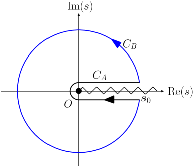
Figure 1: Contour of the integral.

The Weinberg sum rules can be obtained by using the OPE for the second integral. We here consider an asymptotically free theory where the OPE at a UV scale can be done perturbatively. Let ${\cal O}$ be the lowest dimensional operator whose VEV breaks SUSY, and $d$ be the mass dimension (defined by the classical scaling in the UV theory) of ${\cal O}$. Since $\Pi_{D_{1}}$ is dimensionless, it can be expanded as

$$\Pi_{D_{1}}(s)\simeq{c_{\cal O}\langle{\cal O}\rangle\over(-s)^{d/2}}+\cdots,$$ (16)

where $\cdots$ are higher order terms in the $1/(-s)$ expansion and $c_{\cal O}$ is a dimensionless coefficient. Here $d/2$ should be an integer since it can be obtained by a calculation of Feynman diagrams. If $d/2$ is not an integer, such an operator either does not contribute or should be supplied by some dimensionful parameter in the Lagrangian. The second integral in Eq. (15) vanishes for $n<d/2-1$. In general, $d\leq 4$ since $T^{\mu}_{\mu}$ can always be ${\cal O}$.

On the other hand, the function $\Pi_{D_{1}}(s)$ for the real and positive $s$ can be expressed in terms of a spectral function as follows:

$$\Pi_{D_{1}}(s)=-\int_{0}^{\infty}d\sigma^{2}{\rho_{D_{1}}(\sigma^{2})\over s-\sigma^{2}+i\epsilon}+\Delta(s),$$ (17)

where $\Delta(s)$ represents contact terms which are regular everywhere. By using the expression in Eq. (17), the first integral in Eq. (15) reduces to

$$2\pi i\int_{0}^{s_{0}}ds\ s^{n}\rho_{D_{1}}(s)$$ (18)

for $n\geq 0$. For $n<0$, the integral depends on $\Delta(s)$.

In asymptotically free theories, the use of the OPE is justified when $(-s)$ is sufficiently large. Therefore, the quantity (18) should asymptotes to zero for $s_{0}\to\infty$ if $n$ is within the window:

$$0\leq n<{d\over 2}-1.$$ (19)

From $d\leq 4$, such $n$ can only be zero. In summary, we obtain

$$\int_{0}^{\infty}ds\ \rho_{D_{1}}(s)=0,$$ (20)

for models with $d=3$ or $4$.

The sum rules we obtain from $D_{1}$ and $D_{3}$ are

$$\int_{0}^{\infty}ds\ \left(\rho_{1}(s)-\rho_{1/2}(s)\right) = 0,$$ (21)

$$\int_{0}^{\infty}ds\ \left(\rho_{0}(s)-\rho_{1/2}(s)\right) = 0,$$ (22)

where

$$\tilde{C}_{a}(s)=-\int_{0}^{\infty}d\sigma^{2}{\rho_{a}(\sigma^{2})\over s-\sigma^{2}+i\epsilon}.\ \ \ \ (a=0,\ 1/2,\ 1)$$ (23)

No sum rule for $\tilde{B}_{1/2}$ is obtained from other correlators.

2.3 Low energy models and sum rules

Let us assume that the SUSY breaking model is a confining theory and its low-energy physics is well described by the lowest modes à la Weinberg [1]:

$$\rho_{a}(s)=f_{a}^{2}\delta(s-m_{a}^{2}).$$ (24)

In this case, the sum rules Eqs. (21) and (22) suggest

$$f_{0}^{2}=f_{1/2}^{2}=f_{1}^{2}\equiv f^{2}_{h}.$$ (25)

It states that the decay constants are the same even though the masses can split.

By using the formula of the general gauge mediation [4], the scalar masses via gauge mediation are given by

$$m_{s}^{2} = g^{4}c_{2}\int{d^{4}k\over i(2\pi)^{4}}{1\over k^{2}}\left(3\tilde{C}_{1}(k^{2})-4\tilde{C}_{1/2}(k^{2})+\tilde{C}_{0}(k^{2})\right)$$ (26)

$$= {g^{4}c_{2}f^{2}_{h}\over(4\pi)^{2}}\log{m_{0}^{2}m_{1}^{6}\over m_{1/2}^{8}}.$$

Here, $m_{0}$, $m_{1/2}$, $m_{1}$ are masses of the particles with spin 0, 1/2, and 1 in the hidden sector, respectively, and $c_{2}$ is the quadratic Casimir invariant. A finite result is obtained due to the sum rules. (Similar to the $\pi^{+}-\pi^{0}$ mass splitting by QED. See [7].) Interestingly, in Ref. [5], the same expression for the sfermion mass squared was derived in a model with gauge messengers.

From Eqs. (24) and (25), the gaugino masses can also be calculated as

$$m_{\lambda}={g^{2}f^{2}_{h}\over m_{1/2}}.$$ (27)

In summary, by using the sum rules, one can express the sfermion and gaugino masses by hadron masses in the hidden sector.

3 Supercurrent and sum rules

In this section, as another example, we apply the same procedure used in the previous section to the supercurrent multiplet of the SUSY breaking sector.

3.1 Supercurrent and correlators

In a wide class of supersymmetric field theories, one can define a real supermultiplet called the supercurrent ($J^{\mu}$) [8] (See [9] for a recent discussion). It is composed of the SUSY current ($S^{\mu}_{\alpha}$), the symmetric energy momentum tensor ($T^{\mu\nu}$), the $R$-current ($j^{\mu}$), and a scalar operator $x$. The $R$-current defined in this way is not conserved unless the theory is conformal. The transformation laws of those component fields under SUSY are given by

$$\delta_{Q}j_{\mu} = -i\eta\left(S_{\mu}-{1\over 3}\sigma_{\mu}\bar{\sigma}^{\nu}S_{\nu}\right),$$ (28)

$$\delta_{Q}x = -{2\over 3}i\eta\sigma^{\mu}\bar{S}_{\mu},$$ (29)

$$\delta_{Q}x^{\dagger} = 0,$$ (30)

$$\delta_{Q}S_{\mu\alpha} = 2(\sigma_{\mu\nu}\eta)_{\alpha}\partial^{\nu}x^{\dagger},$$ (31)

$$\delta_{Q}\bar{S}_{\mu}^{\dot{\alpha}} = i(\bar{\sigma}^{\nu}\eta)^{\dot{\alpha}}\left[2T_{\mu\nu}+i\partial_{\nu}j_{\mu}-i\eta_{\mu\nu}\partial\cdot j-{1\over 2}\epsilon_{\mu\nu\rho\sigma}\partial^{\rho}j^{\sigma}\right],$$ (32)

$$\delta_{Q}T^{\mu\nu} = -{1\over 2}\left[\eta\sigma^{\rho\mu}\partial_{\rho}S^{\nu}+\eta\sigma^{\rho\nu}\partial_{\rho}S^{\mu}\right].$$ (33)

By using the above component fields, we define the following set of current correlators:

$$C_{1}^{\mu\nu\rho\sigma}(x,y) \equiv \Bigg{\langle}\delta_{Q}^{\alpha}\left[\bar{S}^{\mu\dot{\alpha}}(x)T^{\rho\sigma}(y)\right]\Bigg{\rangle}(\sigma^{\nu})_{\alpha\dot{\alpha}},$$ (34)

$$C_{2}^{\mu\nu\rho\sigma\kappa}(x,y) \equiv \Bigg{\langle}\delta_{Q}^{\alpha}\left[S^{\mu}_{\gamma}(x)T^{\rho\sigma}\right]\Bigg{\rangle}(\sigma^{\nu\kappa})_{\alpha}^{\ \gamma},$$ (35)

$$C_{3}^{\mu\nu}(x,y) \equiv \Bigg{\langle}\delta_{Q}^{\alpha}\left[\bar{S}^{\mu\dot{\beta}}(x)x^{\dagger}(y)\right]\Bigg{\rangle}(\sigma^{\nu})_{\alpha\dot{\beta}},$$ (36)

$$C_{4}^{\mu\nu\kappa}(x,y) \equiv \Bigg{\langle}\delta_{Q}^{\alpha}\left[S^{\mu}_{\gamma}(x)x^{\dagger}(y)\right]\Bigg{\rangle}(\sigma^{\nu\kappa})_{\alpha}^{\ \gamma},$$ (37)

$$C_{5}^{\mu\nu}(x,y) \equiv \Bigg{\langle}\delta_{Q}^{\alpha}\left[\bar{S}^{\mu\dot{\beta}}(x)x(y)\right]\Bigg{\rangle}(\sigma^{\nu})_{\alpha\dot{\beta}},$$ (38)

$$C_{6}^{\mu\nu\kappa}(x,y) \equiv \Bigg{\langle}\delta_{Q}^{\alpha}\left[S^{\mu}_{\gamma}(x)x(y)\right]\Bigg{\rangle}(\sigma^{\nu\kappa})_{\alpha}^{\ \gamma},$$ (39)

$$C_{7}^{\mu\nu\rho}(x,y) \equiv \Bigg{\langle}\delta_{Q}^{\alpha}\left[\bar{S}^{\mu\dot{\beta}}(x)j^{\rho}(y)\right]\Bigg{\rangle}(\sigma^{\nu})_{\alpha\dot{\beta}},$$ (40)

$$C_{8}^{\mu\nu\rho\kappa}(x,y) \equiv \Bigg{\langle}\delta_{Q}^{\alpha}\left[S^{\mu}_{\gamma}(x)j^{\rho}(y)\right]\Bigg{\rangle}(\sigma^{\nu\kappa})_{\alpha}^{\ \gamma}.$$ (41)

If SUSY is unbroken, all of them are vanishing.

Since it will become important when we derive sum rules, let us here discuss $R$-charges associated with the above correlators. The $R$-symmetry plays a crucial role for SUSY breaking [10], and in most cases, it is assumed that UV theories of SUSY breaking models are $R$-symmetric. Therefore, in the present study, we assume that UV theories, from which OPE of the correlators are calculated, have $R$-symmetry. The $R$-charges associated with each correlator are uniquely fixed since the components of the supercurrent have $R$-charges determined from the SUSY algebra. Those are summarized in Table 1,

Correlators	$R$-charge	Dim. of ${\cal O}$
$C_{1},~{}C_{6},~{}C_{7}$	$0$	$d_{0}$
$C_{2},~{}C_{3},~{}C_{5},~{}C_{8}$	$2$	$d_{2}$
$C_{4}$	$4$	$d_{4}$

Table 1: $R$-charges associated with each correlator. $d_{0}$, $d_{2}$ and $d_{4}$ denote the dimension of the lowest-dimension SUSY breaking operator which contribute to the OPE of correlators with $R=0$, $2$ and $4$.

and operators that appear in the OPE of each correlator should have the same $R$-charges as corresponding correlators. If the $R$-symmetry is not broken spontaneously, correlators with non-zero $R$-charges should vanish identically, and only correlators with zero $R$-charge, namely $C_{1}$, $C_{6}$ and $C_{7}$, would provide non-trivial sum rules. Meanwhile, if the $R$-symmetry is spontaneously broken, correlators with non-zero $R$-charges are also non-vanishing, and further sum rules can be derived. For later convenience, we introduce $d_{0}$, $d_{2}$ and $d_{4}$ to denote the dimension of the lowest-dimension SUSY breaking operator which contribute to the OPE of correlators with $R=0$, $2$ and $4$. (See Table 1.) The number of sum rules we can derive from each correlator depends on values of $d_{0,2,4}$ as we will discuss in detail later.

3.2 Sum rules in effective theories

An explicit form of sum rules can be derived by approximating the spectral function by one-particle states of hadrons. Such an approximation is valid when there is a weakly coupled description of hadrons at low energy. We assume that there is such an effective description. As hadronic degrees of freedom, we introduce fields with spins from 0 to 2 as follows:

• $\phi$ (massive or massless spin 0 (scalar)),

• $\pi$ (massive or massless spin 0 (pseudoscalar)),

• $\lambda$ (the Goldstino, spin 1/2, massless),

• $\chi$ (massive spin 1/2 (Majorana)),

• $v_{\mu}$ (massive spin 1 (real)),

• $\psi_{\mu}$ (massive spin 3/2),

• $h^{\mu\nu}$ (massive spin 2).

Except for $\lambda$, there can exist multiple particles with the same spin and parity. In the following, we suppress the indices associated with such multiple particles. The sum rules we obtain below should be understood as the one with summations of these indices.

One particle parts of the supercurrent multiplet can be parametrized as follows:

$$S^{\mu}_{\alpha}=if^{4}\sigma^{\mu}\bar{\lambda}-2f^{2}f^{\prime}\sigma^{\mu\nu}\partial_{\nu}\lambda-2m_{\psi}f_{\psi}\sigma^{\mu\nu}\psi_{\nu}-2f_{\chi}\sigma^{\mu\nu}\partial_{\nu}\chi+\cdots,$$ (42)

$$\bar{S}^{\mu\dot{\alpha}}=if^{4}\bar{\sigma}^{\mu}\lambda-2f^{2}f^{\prime*}\bar{\sigma}^{\mu\nu}\partial_{\nu}\bar{\lambda}-2m_{\psi}f_{\psi}^{*}\bar{\sigma}^{\mu\nu}\bar{\psi}_{\nu}-2f_{\chi}^{*}\bar{\sigma}^{\mu\nu}\partial_{\nu}\bar{\chi}+\cdots,$$ (43)

$$T_{\mu\nu}=-{1\over 2}m_{\rm P}^{2}m_{h}^{2}h_{\mu\nu}-{f_{\phi}\over 2}(\eta_{\mu\nu}\Box-\partial_{\mu}\partial_{\nu})\phi+\cdots,$$ (44)

$$x=c_{\phi}^{2}\phi+ic_{\pi}^{2}\pi+\cdots,$$ (45)

$$j^{\mu}=m_{v}f_{v}v^{\mu}+f_{\pi}\partial^{\mu}\pi+\cdots,$$ (46)

where $\cdots$ are terms which are not linear in fields. The normalization of the fields are such that the propagators are given in Appendix A. We have implicitly assumed the CP invariance, i.e., the absence of the mixing between $\phi$ and $\pi$, for simplicity. By using the above parametrizations and the propagators in Appendix A, one can explicitly calculate the correlators Eqs. (34)-(41) as a sum over the contributions from hadrons.

Following the same procedure in section 2, one can derive the sum rules from $C_{1}-C_{8}$ using the effective theory. For example, we obtain

$$|f^{\prime}|^{2}+|f_{\chi}|^{2}+{2\over 3}|f_{\psi}|^{2}=f_{\phi}^{2}+{8\over 3}m_{\rm P}^{2}$$ (47)

from the correlator $C_{1}$. This rule applies to the models with $d_{0}=3$ and $d_{0}=4$. To derive this rule, we use two approximations; one is the tree level approximation in the effective theory and the other is the perturbative calculation of the OPE for the correlator. The effective theory should have a UV cut-off, $\Lambda_{\rm eff}$, below which the picture of the hadron exchange (tree-level approximation) is justified. On the other hand, the OPE is a good expansion at a sufficiently short distance, $(-s)>\Lambda_{\rm OPE}$, where $\Lambda_{\rm OPE}$ is a typical scale where the UV description breaks down. Therefore, the above sum rule gives a good approximation if $\Lambda_{\rm eff}\gg\Lambda_{\rm OPE}$ and if one takes $s_{0}$ in Fig. 1 within the window, $\Lambda_{\rm OPE}<s_{0}<\Lambda_{\rm eff}$. In the case of QCD, this condition, $\Lambda_{\rm eff}>\Lambda_{\rm OPE}$, seems to be marginally satisfied, therefore the Weinberg’s sum rules are satisfied in the real world to a good accuracy. The hadron summation in the sum rules should be taken while masses exceed $\Lambda_{\rm OPE}$ [11, 12].

Repeating the same discussion for the rest of the correlators, $C_{2}-C_{8}$, we obtain sum rules:

• Boson sum rule ($d_{0}=3$ and $4$)

  $$f_{\phi}^{2}+{8\over 3}m_{\rm P}^{2}=f_{\pi}^{2}+f_{v}^{2},$$ (48)

• Scalar sum rule ($d_{2}=4$)

  $$f_{\phi}c_{\phi}^{2}=0,\ \ \ f_{\pi}c_{\pi}^{2}=0,$$ (49)

• Fermion sum rule ($d_{2}=4$)

  $$f^{2}f^{\prime}=m_{\psi}f_{\psi}^{2}=-{3\over 4}m_{\chi}f_{\chi}^{2}.$$ (50)

The correlator $C_{4}$ does not lead any sum rule for $d_{4}\leq 4$. For $d_{2}>4$ and $d_{4}>4$, there can be more sum rules. However, we do not try to derive those in this paper since we are not aware of such models.

3.3 Improvement of currents and sum rules

The entries in the sum rules, such as $f^{\prime}$, $f_{\chi}$, $f_{\phi}$, and $f_{\pi}$, depend on the definition of the currents in the UV theory. In deriving the sum rules, we have defined the currents as components of the supercurrent multiplet, $J^{\mu}$. Moreover, we have implicitly assumed that the current does not contain parameters with negative mass dimensions, otherwise the dimension of ${\cal O}$ can be arbitrarily small.

If such a supercurrent is uniquely defined, there is no ambiguity for $f$’s. If it is not uniquely defined, the sum rules should hold for any choice of the supercurrents. The supercurrent $J^{\mu}$ has in general a freedom of the improvement,

$$J_{\mu}\to J_{\mu}-\partial_{\mu}(\Omega+\bar{\Omega}),$$ (51)

where $\Omega$ is a chiral superfield. Therefore, the improvement is possible when there is a gauge-invariant chiral superfield with a mass dimension less than or equal to two in the UV theory.

For example, if there is a chiral operator $M$ with dimension two and $R$-charge zero, such as a meson operator, $M$ can be the operator $\Omega$. In the same way as the currents, we parametrize the one-particle parts of the operator $M$ by low energy variables as

$$m = -{i\over\sqrt{2}}\left({F_{\phi}\over\sqrt{2}}\phi-{iF_{\pi}\over\sqrt{2}}\pi\right)+\cdots,$$ (52)

$$\psi_{M\alpha} = -{i\over\sqrt{2}}\left({F^{\prime}}\lambda_{\alpha}+{F_{\chi}}\chi_{\alpha}\right)+\cdots,$$ (53)

$$F_{M} = -i(C_{\phi}^{*2}\phi-iC_{\pi}^{*2}\pi)+\cdots,$$ (54)

where

$$M(y,\theta)=m(y)+\sqrt{2}\theta{\psi_{M}}(y)+\theta\theta F_{M}(y).$$ (55)

With these parametrizations, the improvement in Eq. (51) with $\Omega=cM$, with $c$ a real dimensionless parameter, shifts the decay constants as

$$f^{\prime} \to f^{\prime}+cF^{\prime},$$ (56)

$$f_{\chi} \to f_{\chi}+cF_{\chi},$$ (57)

$$f_{\phi} \to f_{\phi}+cF_{\phi},$$ (58)

$$f_{\pi} \to f_{\pi}+cF_{\pi},$$ (59)

$$c_{\phi}^{2} \to c_{\phi}^{2}+cC_{\phi}^{2},$$ (60)

$$c_{\pi}^{2} \to c_{\pi}^{2}+cC_{\pi}^{2}.$$ (61)

The constants $f$, $f_{v}$, $f_{\psi}$, and $m_{\rm P}$ are unchanged by the improvement.

When $d_{0}\geq 3$, sum rules in Eqs. (47) and (48) should hold for any choice of $c$. Therefore, we obtain the following relations:

$$|F^{\prime}|^{2}+|F_{\chi}|^{2} = F_{\phi}^{2},$$ (62)

$${\rm Re}[f^{\prime*}F^{\prime}]+{\rm Re}[f_{\chi}^{*}F_{\chi}] = f_{\phi}F_{\phi},$$ (63)

$$F_{\phi}^{2} = F_{\pi}^{2},$$ (64)

$$f_{\phi}F_{\phi} = f_{\pi}F_{\pi},$$ (65)

in addition to Eqs. (47) and (48). As a trivial example, the effective theory described by a single chiral superfield,

$$M\propto\phi+i\pi+\sqrt{2}\theta(\lambda{\rm~{}or~{}}\chi)+\theta\theta F,$$ (66)

satisfies the sum rules in Eqs. (62)–(65).

4 UV models and sum rules

In this section, we consider the explicit models of dynamical SUSY breaking and discuss which sum rules in Eqs. (47)–(50) apply to them. Here, we classify those models by whether $R$-symmetry is spontaneously broken, and by dimensions of the SUSY breaking operators.

4.1 Models with unbroken $\boldsymbol{R}$-symmetry

We first discuss the models without spontaneous $R$-symmetry breaking. In this case, the correlators with non-vanishing $R$-charges identically vanish, and thus only Eqs. (47) and (48) can apply. Since $R$-symmetry is not broken, $f^{\prime}=0$ in this case. In most models, $d_{0}=4$ (except for the model with non-vanishing $D$-term for a $U(1)$ factor), and therefore both sum rules apply.

A famous example is the O’Raifeartaigh model [13]. However, in this case, the sum rules do not give new information since one can explicitly derive the low energy models. Examples of dynamical SUSY breaking models are the IYIT model [15, 16] and the ISS model [17] where the ISS model has unbroken discrete $R$-symmetry. Both of the examples have calculable IR descriptions which reduces to the O’Raifeartaigh models.

4.2 Models with spontaneous $\boldsymbol{R}$-symmetry breaking ($d_{2}\leq 3$)

When $R$-symmetry and SUSY are both broken by an operator with $R=2$ and dimension less than four, those models predict the sum rules in (47) and (48).

Examples are incalculable models such as chiral gauge theories in Ref. [2, 3]. There are also possibilities that the incalculable Kähler potential can produce a non-trivial $R$-symmetry breaking vacuum in the vector-like theories such as in [18, 19, 20], although there are known effective descriptions in these cases.

In models of Ref. [2, 3], it is suggested that the gaugino condensation, which has dimension three, breaks both SUSY and the $R$-symmetry through the Konishi anomaly [21]. In the vector-like models in Ref. [18, 19, 20], a dimension-three operator, $\delta_{\bar{Q}\dot{\alpha}}(\bar{\psi}_{S}^{\dot{\alpha}}S)$, is the one which breaks both SUSY and $R$-symmetry, where $\psi_{S}$ and $S$ are the fermionic and the bosonic components of a gauge singlet chiral superfield.

4.3 Models with spontaneous $\boldsymbol{R}$-symmetry breaking ($d_{2}\geq 4$)

Possibly some gauge theory without a matter field can be of this type, although there is no known example. In this case, all the sum rules in Eqs. (47)–(50) can be derived.

Since $R$-symmetry is spontaneously broken, one can say $f_{\pi}\neq 0$. This implies that the left-hand side of Eq. (48) is non-vanishing and therefore the left-hand side of Eq. (47) is also non-vanishing. Together with Eq. (50), $m_{\psi}f_{\psi}^{2}$ is non-vanishing (unless there is a cancellation among same-spin fermions). Therefore, this type of model generally involves massive spin-3/2 field.

If one finds that the sum rules in Eqs. (49) and (50) apply in some hadronic models of SUSY breaking such as the dual gravity constructions [22, 23, 24], it may be suggesting that the microscopic description is in this category.

5 Discussions

We have derived sum rules for hadrons in dynamical SUSY breaking models. The sum rules involve massive fields with spin 3/2 and 2. It is interesting to note here that there is an analogy of this situation in QCD.

The Nambu-Goldstone bosons (pions) associated with the chiral symmetry breaking are described by a non-linear sigma model (chiral Lagrangian) which has a UV cut-off scale. The cut-off scale can be pushed higher by including massive hadrons. The simplest possibility is to promote the non-linear sigma model to a linear-sigma one by introducing a scalar field (which is usually called the sigma meson). However, the actual hadronic world did not choose that realization, instead, a vector meson (the rho meson) appeared as the next lightest state. In view of such situation, the Hidden Local Symmetry (HLS) model [25] is proposed, in which the rho meson is introduced as a massive vector boson of a hidden local SU(2) symmetry.

In SUSY breaking case, the low-energy effective Lagrangian is formulated by Volkov and Akulov in Ref. [26], where the Nambu-Goldstone fermion, the Goldstino, is introduced as non-linearly transforming field under SUSY. The simplest possibility for the next lightest mode is the superpartner of the Goldstino, formulating the low-energy effective model with a chiral supermultiplet. This is analogous to the linear sigma model realization of the chiral symmetry case. As in QCD, it is worth considering an alternative realization, namely the SUSY breaking model equivalent of the HLS realization. Such a realization is achieved by introducing the massive spin-2 field, as discussed in Ref. [27].

Another realization of the massive higher spin states in SUSY gauge theories is related to the gauge/gravity correspondence. For example, in the Holographic QCD model [28, 29, 30, 31], the HLS naturally emerges and the rho meson appears as a “Kaluza-Klein (KK)” excitation mode of the five-dimensional gauge field in the holographic dual. In the context of the gauge/gravity duality, the possibility of the dynamical SUSY breaking has been discussed [22, 23, 24]. If the gravity dual of the dynamical SUSY breaking model is successfully constructed, the Goldstino should be identified with a normalizable zero mode of the KK modes of the bulk gravitino [32]. Furthermore, massive spin-3/2 and massive spin-2 modes also appear from gravitino and graviton in the dual supergravity. In this sense, our effective theory with the hidden local SUSY can be related to the dual supergravity.

Appendix A Propagators

$$\langle\lambda_{\alpha}(x)\bar{\lambda}_{\dot{\beta}}(y)\rangle={1\over f^{4}}\ (\sigma^{\rho})_{\alpha\dot{\beta}}\int{d^{4}k\over i(2\pi)^{4}}{k_{\rho}\over-k^{2}-i\epsilon}e^{-ik\cdot(x-y)}.$$ (67)

$$\langle\chi_{\alpha}(x)\bar{\chi}_{\dot{\beta}}(y)\rangle=(\sigma^{\rho})_{\alpha\dot{\beta}}\int{d^{4}k\over i(2\pi)^{4}}{k_{\rho}\over m_{\xi}^{2}-k^{2}-i\epsilon}e^{-ik\cdot(x-y)}.$$ (68)

$$\langle\chi_{\alpha}(x)\chi^{\beta}(y)\rangle=\delta_{\alpha}^{\beta}\int{d^{4}k\over i(2\pi)^{4}}{m_{\chi}\over m_{\chi}^{2}-k^{2}-i\epsilon}e^{-ik\cdot(x-y)}.$$ (69)

$$\langle\psi_{\mu\alpha}(x)\bar{\psi}_{\nu\dot{\beta}}(y)\rangle=\left(P_{L}\langle\Psi_{\mu}(x)\bar{\Psi}_{\nu}(y)\rangle P_{R}\right)_{\alpha\dot{\beta}}.$$ (70)

$$\langle\psi_{\mu\alpha}(x)\psi_{\nu}^{\beta}(y)\rangle=\left(P_{L}\langle\Psi_{\mu}(x)\bar{\Psi}_{\nu}(y)\rangle P_{L}\right)_{\alpha}^{\ \beta}.$$ (71)

$$\langle\Psi_{\mu}(x)\bar{\Psi}_{\nu}(y)\rangle=\int{d^{4}k\over i(2\pi)^{4}}{P_{\mu\nu}(k)\over m_{\psi}^{2}-k^{2}-i\epsilon}e^{-ik\cdot(x-y)}.$$ (72)

$$P_{\mu\nu}=-\left(\eta_{\mu\nu}-{k_{\mu}k_{\nu}\over m_{\psi}^{2}}\right)\left(\not{k}+m_{\psi}\right)-{1\over 3}\left(\gamma_{\mu}+{k_{\mu}\over m_{\psi}}\right)(\not{k}-m_{\psi})\left(\gamma_{\nu}+{k_{\nu}\over m_{\psi}}\right).$$ (73)

$$\langle h^{\mu\nu}(x)h^{\rho\sigma}(y)\rangle={2\over m_{\rm P}^{2}}\int{d^{4}k\over i(2\pi)^{4}}{B^{\mu\nu;\rho\sigma}\over m_{h}^{2}-k^{2}-i\epsilon}e^{-ik\cdot(x-y)}.$$ (74)

$$B_{\mu\nu;\rho\sigma} = \left(\eta_{\mu\rho}-{k_{\mu}k_{\rho}\over m_{h}^{2}}\right)\left(\eta_{\nu\sigma}-{k_{\nu}k_{\sigma}\over m_{h}^{2}}\right)+\left(\eta_{\mu\sigma}-{k_{\mu}k_{\sigma}\over m_{h}^{2}}\right)\left(\eta_{\nu\rho}-{k_{\nu}k_{\rho}\over m_{h}^{2}}\right)$$ (75)

$$-{2\over 3}\left(\eta_{\mu\nu}-{k_{\mu}k_{\nu}\over m_{h}^{2}}\right)\left(\eta_{\rho\sigma}-{k_{\rho}k_{\sigma}\over m_{h}^{2}}\right).$$

$$\langle\phi(x)\phi(y)\rangle=\int{d^{4}k\over i(2\pi)^{4}}{1\over m_{\phi}^{2}-k^{2}-i\epsilon}e^{-ik\cdot(x-y)}.$$ (76)

$$\langle\pi(x)\pi(y)\rangle=\int{d^{4}k\over i(2\pi)^{4}}{1\over m_{\pi}^{2}-k^{2}-i\epsilon}e^{-ik\cdot(x-y)}.$$ (77)

$$\langle v^{\mu}(x)v^{\nu}(y)\rangle=\int{d^{4}k\over i(2\pi)^{4}}{\eta^{\mu\nu}-{k^{\mu}k^{\nu}/m_{v}^{2}}\over k^{2}-m_{v}^{2}+i\epsilon}e^{-ik\cdot(x-y)}.$$ (78)

References

- [1] S. Weinberg, Phys. Rev. Lett. 18, 507-509 (1967).
- [2] I. Affleck, M. Dine and N. Seiberg, Phys. Lett. B 137, 187 (1984).
- [3] I. Affleck, M. Dine and N. Seiberg, Phys. Lett. B 140, 59 (1984).
- [4] P. Meade, N. Seiberg, D. Shih, Prog. Theor. Phys. Suppl. 177, 143-158 (2009). [arXiv:0801.3278 [hep-ph]].
- [5] K. Intriligator, M. Sudano, JHEP 1006, 047 (2010). [arXiv:1001.5443 [hep-ph]].
- [6] J. F. Fortin, K. Intriligator and A. Stergiou, [arXiv:1109.4940 [hep-th]].
- [7] T. Das, G. S. Guralnik, V. S. Mathur, F. E. Low, J. E. Young, Phys. Rev. Lett. 18, 759-761 (1967).
- [8] S. Ferrara, B. Zumino, Nucl. Phys. B87, 207 (1975).
- [9] Z. Komargodski, N. Seiberg, JHEP 1007, 017 (2010). [arXiv:1002.2228 [hep-th]].
- [10] A. E. Nelson and N. Seiberg, Nucl. Phys. B 416, 46 (1994) [arXiv:hep-ph/9309299].
- [11] M. A. Shifman, A. I. Vainshtein and V. I. Zakharov, Nucl. Phys. B 147, 385 (1979).
- [12] M. A. Shifman, arXiv:hep-ph/0009131; P. Colangelo and A. Khodjamirian, arXiv:hep-ph/0010175.
- [13] L. O’Raifeartaigh, Nucl. Phys. B 96, 331 (1975).
- [14] D. Shih, JHEP 0802, 091 (2008) [arXiv:hep-th/0703196].
- [15] K. I. Izawa and T. Yanagida, Prog. Theor. Phys. 95, 829 (1996) [arXiv:hep-th/9602180].
- [16] K. A. Intriligator and S. D. Thomas, Nucl. Phys. B 473, 121 (1996) [arXiv:hep-th/9603158].
- [17] K. A. Intriligator, N. Seiberg and D. Shih, JHEP 0604, 021 (2006) [arXiv:hep-th/0602239].
- [18] Z. Chacko, M. A. Luty and E. Ponton, JHEP 9812, 016 (1998) [arXiv:hep-th/9810253].
- [19] T. Hotta, K. I. Izawa and T. Yanagida, Phys. Rev. D 55, 415 (1997) [arXiv:hep-ph/9606203].
- [20] M. Ibe and R. Kitano, Phys. Rev. D 77, 075003 (2008) [arXiv:0711.0416 [hep-ph]].
- [21] K. Konishi, Phys. Lett. B135, 439 (1984).
- [22] S. Kachru, J. Pearson and H. L. Verlinde, JHEP 0206, 021 (2002) [arXiv:hep-th/0112197].
- [23] R. Argurio, M. Bertolini, S. Franco and S. Kachru, JHEP 0701, 083 (2007) [arXiv:hep-th/0610212].
- [24] R. Argurio, M. Bertolini, S. Franco and S. Kachru, JHEP 0706, 017 (2007) [AIP Conf. Proc. 1031, 94 (2008)] [arXiv:hep-th/0703236].
- [25] M. Bando, T. Kugo, S. Uehara, K. Yamawaki, T. Yanagida, Phys. Rev. Lett. 54, 1215 (1985).
- [26] D. V. Volkov, V. P. Akulov, JETP Lett. 16, 438-440 (1972).
- [27] M. L. Graesser, R. Kitano and M. Kurachi, JHEP 0910, 077 (2009) [arXiv:0907.2988 [hep-ph]].
- [28] D. T. Son, M. A. Stephanov, Phys. Rev. D69, 065020 (2004). [hep-ph/0304182].
- [29] T. Sakai, S. Sugimoto, Prog. Theor. Phys. 113, 843-882 (2005). [arXiv:hep-th/0412141 [hep-th]].
- [30] J. Erlich, E. Katz, D. T. Son, M. A. Stephanov, Phys. Rev. Lett. 95, 261602 (2005). [hep-ph/0501128].
- [31] L. Da Rold, A. Pomarol, Nucl. Phys. B721, 79-97 (2005). [hep-ph/0501218].
- [32] R. Argurio, G. Ferretti and C. Petersson, JHEP 0603, 043 (2006) [arXiv:hep-th/0601180].