Galaxy And Mass Assembly (GAMA): The galaxy stellar mass function at $\mathbf{z<0.06}$.

Abstract

We determine the low-redshift field galaxy stellar mass function (GSMF) using an area of 143 deg² from the first three years of the Galaxy And Mass Assembly (GAMA) survey. The magnitude limits of this redshift survey are $r<19.4$ mag over two thirds and 19.8 mag over one third of the area. The GSMF is determined from a sample of 5210 galaxies using a density-corrected maximum volume method. This efficiently overcomes the issue of fluctuations in the number density versus redshift. With $H_{0}=70{\rm\,km\,s^{-1}\,Mpc^{-1}}$, the GSMF is well described between $10^{8}$ and $10^{11.5}{\rm M}_{\odot}$ using a double Schechter function with ${\cal M}^{*}=10^{10.66}{\rm M}_{\odot}$, $\phi_{1}^{*}=3.96\times 10^{-3}{\rm\,Mpc}^{-3}$, $\alpha_{1}=-0.35$, $\phi_{2}^{*}=0.79\times 10^{-3}{\rm\,Mpc}^{-3}$ and $\alpha_{2}=-1.47$. This result is more robust to uncertainties in the flow-model corrected redshifts than from the shallower Sloan Digital Sky Survey main sample ($r<17.8$ mag). The upturn in the GSMF is also seen directly in the $i$-band and $K$-band galaxy luminosity functions. Accurately measuring the GSMF below $10^{8}{\rm M}_{\odot}$ is possible within the GAMA survey volume but as expected requires deeper imaging data to address the contribution from low surface-brightness galaxies.

1 Introduction

The galaxy luminosity function (GLF) is a fundamental measurement that constrains how the Universe’s baryonic resources are distributed with galaxy mass. Before the advent of CCDs and near-IR arrays, the GLF had been primarily measured in the $B$-band (Felten 1977; Binggeli, Sandage, & Tammann 1988; Efstathiou, Ellis, & Peterson 1988; Loveday et al. 1992). More recently the low-redshift GLF has been measured using thousands of galaxies in the redder visible bands (Brown et al., 2001; Blanton et al., 2003b) and the near-IR (Cole et al., 2001; Kochanek et al., 2001), which more closely follows that of the underlying galaxy stellar mass function (GSMF). Furthermore the increased availability of multi-wavelength data and spectra enables stellar masses of galaxies to be estimated using colours (Larson & Tinsley, 1978; Jablonka & Arimoto, 1992; Bell & de Jong, 2001) or spectral fitting (Kauffmann et al. 2003; Panter, Heavens, & Jimenez 2004; Gallazzi et al. 2005), and either of these methods allow the GSMF to be computed (Salucci & Persic 1999; Balogh et al. 2001; Bell et al. 2003; Baldry, Glazebrook, & Driver 2008, hereafter, BGD08).

Measurement of the GSMF has now become a standard tool to gain insights into galaxy evolution with considerable effort to extend analyses to $z\sim 1$ (Drory et al., 2009; Pozzetti et al., 2010; Gilbank et al., 2011; Vulcani et al., 2011) and higher (Elsner, Feulner, & Hopp 2008; Kajisawa et al. 2009; Marchesini et al. 2009; Caputi et al. 2011; González et al. 2011; Mortlock et al. 2011). Overall the cosmic stellar mass density is observed to grow by a factor of 10 between $z\sim 2$–3 and $z=0$ (Dickinson et al., 2003; Elsner et al., 2008) with significantly less relative growth in massive $>10^{11}{\rm M}_{\odot}$ galaxies since $z\sim 1$–2 (Wake et al., 2006; Pozzetti et al., 2010; Caputi et al., 2011). The evolution in the GSMF is uncertain, however, with some authors suggesting there could be evolution in the stellar initial mass function (IMF) (Davé, 2008; Wilkins et al., 2008; van Dokkum, 2008) and considering the range of uncertainties associated with estimating stellar masses (Maraston et al. 2006; Conroy, Gunn, & White 2009).

The observed GSMF, defined as the number density of galaxies per logarithmic mass bin, has a declining distribution with mass with a sharp cutoff or break at high masses often fitted with a Schechter (1976) function. At low redshift, the characteristic mass of the Schechter break has been determined to be between $10^{10.6}$ and $10^{11}{\rm M}_{\odot}$ (Panter et al. 2007; BGD08; Li & White 2009). The GSMF shape, however, is not well represented by a single Schechter function with a steepening below $10^{10}{\rm M}_{\odot}$ giving rise to a double Schechter function shape overall (BGD08). Peng et al. (2010b) note that this shape arises naturally in a model with simple empirical laws for quenching of star formation in galaxies. This is one example of the potential for insights that can be obtained by studying the inferred GSMF as opposed to comparing observations and theoretical predictions of the GLF; though we note that it is in some sense more natural for theory to predict the GLF because model galaxies have a ‘known’ star-formation history.

Abundance matching between a theoretical galactic halo mass function and a GLF or GSMF demonstrates that, in order to explain the GSMF shape, the fraction of baryonic mass converted to stars increases with mass to a peak before decreasing (Marinoni & Hudson 2002; Shankar et al. 2006; BGD08; Conroy & Wechsler 2009; Guo et al. 2010; Moster et al. 2010). Galaxy formation theory must explain the preferred mass for star formation efficiency, the shallow low-mass end slope compared to the halo mass function, and the exponential cutoff at high masses (Oppenheimer et al., 2010). At high masses, feedback from active galactic nuclei has been invoked to prevent cooling of gas leading to star formation (Best et al., 2005; Kereš et al., 2005; Bower et al., 2006; Croton et al., 2006). The preferred mass scale may correspond to a halo mass of $\sim 10^{12}{\rm M}_{\odot}$ above which gas becomes more readily shock heated (Dekel & Birnboim, 2006). Toward lower masses, supernovae feedback creating galactic winds is thought to play a major role in regulating star formation (Larson, 1974; Dekel & Silk, 1986; Lacey & Silk, 1991; Kay et al., 2002); while Oppenheimer et al. have argued that it is re-accretion of these winds that is critical in shaping the GSMF. Others have argued that star formation in the lowest mass haloes is also suppressed by photoionization (Efstathiou, 1992; Thoul & Weinberg, 1996; Somerville, 2002), in particular, to explain the number of satellites in the Local Group (Benson et al., 2002).

Recently, Guo et al. (2011) used a semi-analytical model applied to the Millenium Simulation (MS) (Springel et al., 2005) and the higher resolution MS-II (Boylan-Kolchin et al., 2009) to predict the cosmic-average ‘field’ GSMF down to $10^{6}{\rm M}_{\odot}$. They find that the GSMF continues to rise to low masses reaching $>0.1$ galaxies per Mpc³ for $10^{6}$–$10^{7}{\rm M}_{\odot}$, however, they caution that their model produces a larger passive fraction than is observed amongst the low-mass population. Mamon et al. (2011) apply a simple one-equation prescription, on top of a halo merger tree, that requires star formation to occur within a minimum mass set by the temperature of the inter-galactic medium. Their results give a rising baryonic mass function down to $10^{5.5}{\rm M}_{\odot}$, with the peak of the mass function of the star-forming galaxy population at $\sim 10^{7}{\rm M}_{\odot}$. We note that it is useful for theorists to predict the field GSMF of the star-forming population because measuring this to low masses, while challenging, is significantly easier than for the passive population.

Measurements of the GLF reaching low luminosities have been made for the Local Group (Koposov et al., 2008), selected groups (Trentham & Tully, 2002; Chiboucas, Karachentsev, & Tully, 2009), clusters (Sabatini et al., 2003; Rines & Geller, 2008) and superclusters (Mercurio et al., 2006). To accurately measure the cosmic-average GSMF, it is necessary to survey random volumes primarily beyond $\sim 10$ Mpc because: (i) at smaller distances, the measurement is limited in accuracy by systematic uncertainties in distances to galaxies (Masters, Haynes, & Giovanelli, 2004); and (ii) a local volume survey is significantly biased, e.g., the $B$-band luminosity density out to 5 Mpc is about a factor of 5 times the cosmic average (using data from Karachentsev et al. 2004 in comparison with Norberg et al. 2002; Blanton et al. 2003b). The Sloan Digital Sky Survey (SDSS) made a significant breakthrough with redshifts obtained to $r<17.8$ mag and multi-colour photometry (Stoughton et al., 2002), in particular, with the low-redshift sample described by Blanton et al. (2005a). In order to extend and check the low-mass GSMF (BGD08), it is necessary to go deeper over a still significant area of the sky.

Here we report on the preliminary analysis to determine the $z<0.06$ GSMF from the Galaxy And Mass Assembly (GAMA) survey, which has obtained redshifts to $r<19.8$ mag currently targeted using SDSS imaging but which ultimately will be updated with deeper imaging. The plan of the paper is as follows. In § 2, the data, sample selection and methods are described; in § 3, the GLF and GSMF results are presented and discussed. Summary and conclusions are given in § 4.

Magnitudes are corrected for Galactic extinction using the dusts maps of Schlegel, Finkbeiner, & Davis (1998), and are $k$-corrected to compute rest-frame colours and absolute magnitudes using kcorrect v4_2 (Blanton et al., 2003a; Blanton & Roweis, 2007). We assume a flat $\Lambda$CDM cosmology with $H_{0}=70{\rm\,km\,s^{-1}\,Mpc^{-1}}$ and $\Omega_{m,0}=0.3$. The Chabrier (2003) IMF (similar to the Kroupa 2001 IMF) is assumed for stellar mass estimates. Solar absolute magnitudes are taken from table 1 of Hill et al. (2010), and mass-to-light ratios are given in solar units.

2 Data and methods

2.1 Galaxy And Mass Assembly survey

The GAMA survey aims to provide redshifts and multi-wavelength images of $>250$ 000 galaxies over $>250\,{\rm deg}^{2}$ to $r<19.8$ mag (Driver et al., 2009, 2011; Baldry et al., 2010). A core component of this programme is a galaxy redshift survey using the upgraded 2dF instrument AAOmega (Sharp et al., 2006) on the Anglo-Australian Telescope. The first three years of the redshift survey have been completed (Driver et al., 2011) and these data are used here. The target selection was over three $48\,{\rm deg}^{2}$ fields centred at 9 h (G09), 12 h (G12) and 14.5 h (G15) on the celestial equator. The limiting magnitudes of the main survey were $r<19.4$ in G09 and G15, $r<19.8$ in G12, $z<18.2$ and $K_{\rm AB}<17.6$ (Baldry et al., 2010). It is only the $r$-band selection that is used in the current analysis because the near-IR selections add mainly higher-redshift galaxies. Each area in the survey was effectively ‘tiled’ 5–10 times with a strategy aiming for high completeness (Robotham et al., 2010). In other GAMA papers, Loveday et al. (2012) determines the $ugriz$ GLFs, Driver et al. (2012) determines the cosmic spectral energy distribution from the far ultraviolet to infrared, while Brough et al. (2011) looks at the properties of galaxies at the faint end of the H$\alpha$ GLF.

The target selection was based primarily on SDSS DR6 (Adelman-McCarthy et al., 2008) with the $K$-band selection using UKIRT Infrared Deep Sky Survey (UKIDSS, Lawrence et al. 2007), and star-galaxy separation using both surveys (see Baldry et al. 2010 for details). Quality control of the imaging selection was done prior to the redshift survey to remove obvious artifacts and deblended parts of galaxies. An update to the target list was performed to remove targets with erroneous selection photometry (§ 2.9 of Driver et al. 2011). For this paper, further visual inspection was made of low-redshift ‘pairs’ with measured velocity differences $<300{\rm\,km\,s^{-1}}$. This resulted in $\sim 50$ objects being reclassified as a deblended part of a galaxy. Further inspection was made of targets with faint fibre magnitudes, reclassifying $\sim 100$ objects as not a target. After this, the $r$-band magnitude limited main survey consists of 114 360 targets.

Various photometric measurements are used in this paper. The selection magnitudes are SDSS Petrosian magnitudes from the photo pipeline (Stoughton et al., 2002). In order to obtain matched aperture photometry from $u$- to $K$-band, the imaging data from SDSS and UKIDSS were reprocessed and run through SExtractor (Bertin & Arnouts, 1996). The details are given in Hill et al. (2011) and here we use the $r$-defined auto magnitudes primarily for colours: these use elliptical apertures. SExtractor fails to locate some genuine sources that were identified by photo, however, and for these we use Petrosian colours. Finally, an estimate of total luminosity is obtained using Sersic fits extrapolated to 10$R_{e}$ (ten times the half-light radius). This procedure uses a few software packages including galfit ver. 3 (Peng et al., 2010a) and is described in detail by Kelvin et al. (2011).

Spectra for the GAMA survey are taken with the AAOmega spectrograph on the Anglo-Australian Telescope (AAT), coupled with various other public survey data and some redshifts from the Liverpool Telescope. The AAT data were reduced using 2dFdr (Croom, Saunders, & Heald, 2004) and the redshifts determined using runz (Saunders, Cannon, & Sutherland, 2004). The recovered redshift for each spectrum is assigned a quality $Q$ from 1 (no redshift) to 4 (reliable). These are later updated based on a comparative analysis between different opinions of a large subset of spectra. From this process, a best redshift estimate and the probability ($p_{z}$) of whether this is correct are assigned to each spectrum. The new $Q$ values are based on these probabilities (formally called $nQ$, § 2.5 of Driver et al. 2011). Where there is more than one spectrum for a source, the redshift is taken from the spectrum with the highest $Q$ value. For the $r$-band limited main sample, 93.1%, 3.0% and 3.4% have $Q\geq 4$, $Q=3$ and $Q=2$, respectively. In general, redshifts with $Q\geq 3$ are used, however, $Q=2$ can be considered when there is agreement with a second spectrum that was measured independently or when there is reasonable agreement with an independent photometric redshift estimate.

2.2 Stellar mass estimates

Stellar masses were computed for GAMA targets using the observed auto matched aperture photometry (Hill et al., 2011) for the $ugriz$ bands. These were fitted using a grid of synthetic spectra with exponentially declining star formation histories produced using Bruzual & Charlot (2003) models with the Chabrier (2003) IMF and the Calzetti et al. (2000) dust obscuration law. The stellar masses were determined from probability weighted integrals over the full range of possibilities provided by the grid. See Taylor et al. (2011) for details of the method. For the fitted stellar masses in this paper, we use the stellar mass-to-light ratios (M/L) in $i$-band applied to the $i$-band Sersic fluxes. Where M/L values are not available (2% of the low-redshift sample), we use the colour-based relation of Taylor et al. (2011) to estimate M/L_i.

The 95% range in M/L_i from the fitting by Taylor et al. (2011) is 0.5–2.0 (${\rm M}_{\odot}/{\rm L}_{\odot}$) for high luminosity galaxies ($L_{i}>10^{10}{\rm L}_{\odot}$) and 0.2–1.6 for lower luminosity galaxies ($z<0.06$). The net uncertainty on an individual stellar mass estimate can be large, e.g., a factor of two or 0.3 dex as estimated by Conroy et al. (2009). Note though that the impact of uncertainties is more important when considering evolution in the GSMF than when considering the shape of the GSMF at a single epoch as in this paper. The latter primarily depends on the differential systematic uncertainty between populations. Taylor et al. (2010a) estimated that the net differential bias was $\la 0.12{\rm\,dex}$ based on comparing stellar and dynamical mass estimates. The change in M/L_i between red and blue galaxy populations can be approximated by a colour-based M/L relation. The effect of changing the slope of this relation is considered in § 3.3.

We note that the reason that M/L correlates with colour at all well is that the M/L of a stellar population increases as a population reddens with age or dust attenuation. Bell & de Jong (2001) noted that errors in dust estimates do not strongly affect stellar mass estimates. In other words, the vectors in M/L versus dust reddening run nearly parallel to those determined for age reddening. Driver et al. (2007), using the dust models of Popescu et al. (2000) and Tuffs et al. (2004), confirmed this with the largest deviation for edge-on systems.

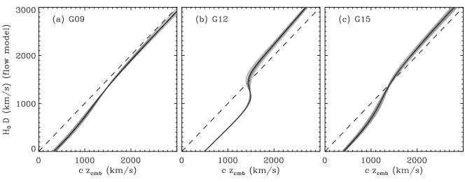
Figure 1: The relation between distance and CMB-frame redshift from the Tonry et al. (2000) flow model. The three GAMA regions are shown in different panels. The black line represents the central sight line while the grey region shows the variation over each GAMA region.

2.3 Distances

The GAMA survey, as with most large redshift surveys, provides the heliocentric redshift as standard. In many cases it is sufficient to assume that this is close to the cosmological redshift. For the GAMA regions at low redshift, however, it is not.

First we convert heliocentric redshifts to the cosmic microwave background (CMB) frame:

$$1+z_{\rm cmb}=(1+z_{\rm helio})(1+z_{\rm sun,comp})$$ (1)

where $c\,z_{\rm sun,comp}$ is the component of the Sun’s velocity toward the object in the CMB frame. We use $z_{\rm sun}=0.001231$ ($369{\rm\,km/s}$) for the CMB dipole in the direction of ${\rm RA}=168.0\degr$ and ${\rm DEC}=-7.2\degr$ (Lineweaver et al., 1996). For the GAMA survey, this leads to average corrections for the heliocentric velocity ($c\,z_{\rm sun,comp}$) of $+303$, $+357$ and $+236{\rm\,km\,s^{-1}}$, in G09, G12 and G15, respectively.

In the absence of flow information, the CMB frame redshift is a preferred estimate of the cosmological redshift at $z>0.03$; the velocity of the Local Group (LG) with respect to the CMB has been attributed to superclusters at lower redshifts (Tonry et al., 2000; Erdoğdu et al., 2006). However, it should be noted that large-scale bulk flows have been claimed by, for example, Watkins, Feldman, & Hudson (2009). To account for flows in the nearby Universe, we use the flow model of Tonry et al. linearly tapering to the CMB frame between $z=0.02$ and $z=0.03$. Figure 1 shows the relation between the flow-corrected and CMB frame velocity at $z<0.01$. The main feature is the difference between velocities in front of and behind the Virgo Cluster for sight lines in G12. For each object sky position, the flow-corrected redshift is obtained by computing the model CMB frame redshifts ($z_{\rm cmb,m}$) for a vector of cosmological redshifts ($z_{\rm m}$ from $-1000$ to $+1000{\rm\,km\,s^{-1}}$ in steps of 10 around the observed $z_{\rm cmb}$). The flow-corrected redshift ($z$) is then given by the weighted mean of $z_{\rm m}$ values with weights

$$w_{m}=\exp\left(\frac{-(z_{\rm cmb,m}-z_{\rm cmb})^{2}}{2\sigma^{2}}\right)$$ (2)

where $\sigma$ is taken as $50{\rm\,km\,s^{-1}}$. This small value is chosen so that the result is nearly equivalent to using the one-to-one solution for flow-corrected redshift from $z_{\rm cmb}$, which is mostly available, and it corresponds to a typical redshift uncertainty from the GAMA spectra (Driver et al., 2011). It is only around $1500{\rm\,km/s}$ in G12 where the method is necessary to provide a smoothly varying weighted average between the three solutions.

Figure 2(a) shows the difference in distance modulus (DM) using the flow-corrected $z$ compared to using $z_{\rm helio}$ versus redshift. Note that the correction to a DM can be larger than 0.5 mag; the direction of G12 in particular is within $20\degr$ of both the CMB dipole and the Virgo Cluster (cf. fig. 5 of Jones et al. 2006 for the Southern sky). The DM uncertainty for each galaxy was estimated by applying changes in heliocentric velocity of $\pm 180{\rm\,km/s}$ and recomputing the flow-corrected distances. This corresponds to the cosmic thermal velocity dispersion in the Tonry et al. (2000) model, i.e., the velocity deviations after accounting for the attractors. Figure 2(b) shows the DM uncertainties, which are taken as half the difference between the positive and negative changes. The uncertainty is less than 0.2 mag at $z>0.007$, while at the lower redshifts the uncertainty can be quite large especially in G12 because of the triple-valued solution caused by Virgo infall [Fig. 1(b)].

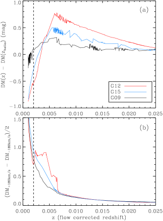
Figure 2: (a): The difference in the distance moduli derived from $z$ and $z_{\rm helio}$. The lines connect the locations of the galaxies for each region, which have been sorted by redshift. The vertical dashed line shows the low-redshift limit for the further analyses in this paper. (b): An estimate of the uncertainty in the the distance moduli. The distance moduli were recomputed after adjusting the heliocentric redshift by $\pm 180{\rm\,km\,s^{-1}}$ and half this difference is plotted.

To show the significance of using different distances, the $r$-band GLF was computed using these flow-corrected redshifts, heliocentric frame, LG frame (Courteau & van den Bergh, 1999) and CMB frame (Lineweaver et al., 1996). Figure 3 shows the 4 resultant GLFs. The computed number densities are significantly different at magnitudes fainter than $\sim-15$ because of variations in the estimated absolute magnitudes, the sample, and the volumes $V_{\rm max}$. The estimates of number density are lower when using the flow-corrected redshifts or CMB frame, with respect to heliocentric or LG frame, because of larger distances and thus higher luminosities with lower $1/V_{\rm max}$ weighting. Masters et al. (2004) noted that the Tonry et al. (2000) model works well toward Virgo although possibly at the expense of the anti-Virgo direction, but in any case, the model is suitable for the GAMA fields. Hereafter, we use the Tonry et al. flow-corrected redshifts.

Figure 3: Comparison between galaxy luminosity functions computed using different approximations for the cosmological redshift. The samples were selected over the redshift range 0.003 to 0.06, and a standard $V_{\rm max}$ method was used. The solid line with error bars shows the GLF using the flow-corrected distances (offset $\times 0.2$, also shown with no offset without error bars).

2.4 Sample selection

In addition to the survey selection described in Baldry et al. (2010), the sample selection is as follows:

1. $r_{\rm Pet}<19.4$ mag in G09 or G15, or $r_{\rm Pet}<19.8$ mag in G12;

2. redshift quality $Q\geq 3$, $Q=2$ when there was agreement with a second independent spectrum of the same target (within a velocity difference of $450{\rm\,km\,s^{-1}}$), or $Q=2$ with $p_{z}>0.7$ and agreement with a photometric redshift estimate [within 0.05 in $\delta z/(1+z)$];

3. $0.002<z<0.06$ (flow corrected), comoving distances from 8.6 Mpc to 253 Mpc;

4. physical Petrosian half-light radius $>$ 100 pc.

The magnitude limits define the $r$-band limited main sample (114 360) with 98.3% (112 393) satisfying the redshift quality criteria. The redshift range reduces the sample to 5217 (50 of these were included because of the $Q=2$ agreement tests). A further 7 sources are rejected by the half-light radius criterium giving a primary sample of 5210 galaxies. The 100 pc lower limit corresponds to Gilmore et al. (2007)’s division between star clusters and galaxies. However, on inspection the rejected sources were simply assigned an incorrect redshift and should be either stellar or at higher redshift than our sample limit.

Figure 4 shows the distribution of the primary sample in $M_{r}$ versus redshift. Note not all the redshifts come from the GAMA AAOmega campaign with the breakdown as follows: 2671 GAMA, 2007 SDSS, 444 2dF Galaxy Redshift Survey, 64 Millennium Galaxy Catalogue, 10 6dF Galaxy Survey, 6 Updated Zwicky Catalogue, 6 Liverpool Telescope, and 2 others via the NASA/IPAC Extragalactic Database.

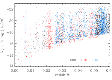
Figure 4: Absolute magnitude versus redshift. The black and blue points represent galaxies in G09 and G15 to $r<19.4$ while the red points represent galaxies in G12 to $r<19.8$.

The Petrosian photometry, used for selection of the sample, is highly reliable having undergone various visual checks. The exception is for overdeblended sources. For these the deblended parts have been identified and associated with a target galaxy. The $r$-band Petrosian photometry of these overdeblended sources is recomputed by summing the flux from identified parts. About 100 galaxies have their Petrosian magnitude brightened by $>0.1$ mag from this, with 14 brightened by more than a magnitude (the target part has not been assigned the majority of flux in a few cases). It is important to do this prior to calculating $V_{\rm max}$ because a nearby galaxy that is deblended into parts would not be deblended nearly so significantly if placed at higher redshift.

2.5 Density-corrected maximum volume method

A standard method to compute binned GLFs is through weighting each galaxy by $1/V_{\rm max}$ (Schmidt, 1968), which is the comoving volume over which the galaxy could be observed within the survey limits ($z_{\rm max}$ is the corresponding maximum redshift). In the presence of large-scale structure, large variations in the number density versus redshift, this method can distort the shape of the GLF (Efstathiou et al., 1988). Figure 5 shows the large-scale structure in and around the GAMA regions. There are a few substantial overdensities and underdensities as a function of redshift within each region.

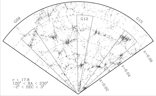
Figure 5: Redshift distribution in and around the GAMA regions. Only galaxies with $r<17.8$ are shown corresponding to the SDSS main galaxy sample limit (but including redshifts from all surveys). Note the low number of galaxies at low RA, to the left of G09 in this figure, is because of the lack of redshift survey coverage from SDSS, 2dFGRS and GAMA.

In order to compute binned GLFs undistorted by radial variations in large-scale structure, a density-corrected $V^{\prime}_{\rm max}$ method is used. This is given by

$$\phi_{\log L}=\frac{1}{\Delta\log L}\,\sum_{i}\frac{1}{V^{\prime}_{{\rm max},i}\,c_{i}}$$ (3)

where $c_{i}$ is the completeness factor assigned to a galaxy; and the corrected volume is given by

$$V^{\prime}_{{\rm max},i}=\frac{\rho_{\rm ddp}(z_{1};z_{{\rm max},i})}{\rho_{\rm ddp}(z_{1};z_{2})}\>V_{{\rm max},i}$$ (4)

where $\rho_{\rm ddp}(z_{a};z_{b})$ is the number density of a density-defining population (DDP) between redshifts $z_{a}$ and $z_{b}$, $z_{1}=0.002$ is the low-redshift limit, and $z_{2}=0.06$ is the high-redshift limit of the sample. This method is also described in § 2.7 of Baldry et al. (2006) where the density-corrected volume is given by $f_{V}V_{\rm max}$. To calculate this, we first treat G09+G15 and G12 separately because of the different magnitude limits, except that we use a single value for $\rho_{\rm ddp}(z_{1};z_{2})$, which is taken to be the average density of the DDP over all three regions. The DDP must be a volume-limited sample and we use $M_{r}<-17.9$ (Fig. 4). Figure 6 shows the relative number density [$f_{V}(z)=\rho_{\rm ddp}(z_{1};z)/\rho_{\rm ddp}(z_{1};z_{2})$] for the separate samples.

Figure 6: Variation in number density of the DDP used in the density-corrected $V^{\prime}_{\rm max}$ method. The lines represent the number density of the $M_{r}<-17.9$ volume-limited sample divided by $0.0148{\rm\,Mpc}^{-3}$ from $z=0.002$ up to the redshift shown on the $x$-axis.

The redshift upper limit of 0.06 allows sufficient statistics to be obtained at the bright end to fit the knee of the GLF or GSMF while at the same time allowing the use of a single DDP that can be used to reliably measure $V^{\prime}_{\rm max}$ for galaxies as faint as $M_{r}\sim-13$. Raising the redshift limit to 0.1 would improve the bright-end statistics at the expense of using a DDP with a limit that is 1.1 mag brighter, which is less accurate for determining $V^{\prime}_{\rm max}$ values. We note, however, that it is possible to use a series of overlapping volume-limited samples to improve the accuracy of $V^{\prime}_{\rm max}$ (e.g. Mahtessian 2011 ‘sewed’ three samples together). For the purposes of keeping a simple transparent assumption and mitigating against even modest evolution, for this paper we use a single DDP with $z<0.06$.

The step-wise maximum likelihood (SWML) (Efstathiou et al., 1988) method can also be used to compute a binned GLF that is not distorted by large-scale structure variations. In fact, computing the density binned radially and the binned GLF using a maximum likelihood method can be shown to be equivalent to a density-corrected $V^{\prime}_{\rm max}$ method (§ 8 of Saunders et al. 1990; Cole 2011). This is reassuring but not surprising given that both SWML and density-corrected $V^{\prime}_{\rm max}$ methods assume that the shape of the GLF remains the same between different regions. This is not exactly true but the resulting GLF is a weighted radial average. This is seen more transparently in the density-corrected $V^{\prime}_{\rm max}$ method. The real advantage here is that $V^{\prime}_{\rm max}$ need only be calculated for each galaxy using the selection $r$-band Petrosian magnitudes after which the GLF (or GSMF) can be determined straightforwardly using different photometry. When calculating the GLF in a different band (or the GSMF) there is no colour bias in a bin unless a population with a certain colour is only visible over a reduced range of luminosity (mass) within the bin. Note also the GAMA DDP sample is highly complete, which means that the calculation of $\rho_{\rm ddp}$ is robust.

Figure 7 shows a comparison between $V^{\prime}_{\rm max}$ and $V_{\rm max}$. For example, note the flattening of $V^{\prime}_{\rm max}$ in G12 brighter than $-15.2$ (red line). This corresponds to the overdensity at $z\simeq 0.022$ with the underdensity beyond. Brighter galaxies can be seen further but the corrected volume rises slower than the standard $V_{\rm max}$ because the DDP is underdense beyond.

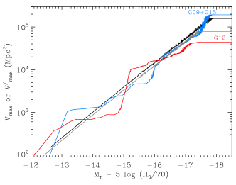
Figure 7: Comparison between standard maximum volumes and corrected volumes. The black and grey lines represent $V_{\rm max}$; note the small scatter is due to differential $k$-corrections between $z$ and $z_{\rm max}$. The blue and red lines represent $V^{\prime}_{\rm max}$. A minimum value of $100{\,\rm Mpc^{3}}$ was set for $V^{\prime}_{\rm max}$ because this volume could only be expected to contain typically 1 or 2 galaxies of the DDP.

In order to estimate GLFs, the completeness is assumed to be unity ($c_{i}=1$) in this paper with the area of the survey being $143\,{\rm deg}^{2}$ (one third of this for each region). Figure 8 shows the $i$-band GLF computed using the different volume correction methods. The $V^{\prime}_{\rm max}$ method produces much better agreement between the regions than the standard $V_{\rm max}$ method. The remaining difference between the regions, below $<10^{8}{\rm L}_{\odot}$ in particular, may be the result of the GLF varying between environments or uncertainties in the distances. The grey lines in Fig. 8 represent the GLF using a combined volume over all regions. This is obtained by modifying $\rho_{\rm ddp}(z_{1};z_{{\rm max},i})\,V_{{\rm max},i}$ in Eq. 4 to be a sum over all three regions for each galaxy with $z_{{\rm max},i}$ being different in G09+G15 ($r<19.4$) compared to G12 ($r<19.8$) (see also Avni & Bahcall 1980 for combining samples with different effective volumes). Hereafter, this combined $V^{\prime}_{\rm max}$ is used. Note also we show GLFs using solar luminosities because we are working towards the GSMF.

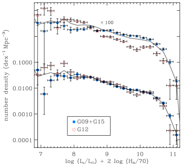
Figure 8: Comparison between the standard $V_{\rm max}$ (upper data) and density-corrected $V^{\prime}_{\rm max}$ (lower data) for determining the $i$-band GLF. The triangles show the GLFs from the standard method (offset $\times 100$). Note the major discrepancies between the regions. The circles show the GLFs from the $V^{\prime}_{\rm max}$ method. The grey lines (no offset and offset $\times 100$) represent the GLF using a combined $V^{\prime}_{\rm max}$ over all three regions.

3 Results and discussion

3.1 Galaxy luminosity functions in the $i$-band

The S/N in the $i$-band is significantly higher than the SDSS $z$-band or any of the UKIDSS bands for galaxies in our sample. Thus we use the $i$-band as the fiducial band from which to apply stellar mass-to-light ratios. First we start by looking at the $i$-band and comparing the GLF taken with different photometric apertures. Figure 9(a) shows the $i$-band GLF using photometry from (i) SDSS pipeline photo, (ii) SExtractor as run by Hill et al. (2011) and (iii) galfit as run by Kelvin et al. (2011). For comparison, the result from Loveday et al. (2012) at $z<0.1$ using Petrosian magnitudes and SWML method is also shown (here computed slightly differently to their paper, with $k$-corrections to $z=0$ and with no completeness corrections).

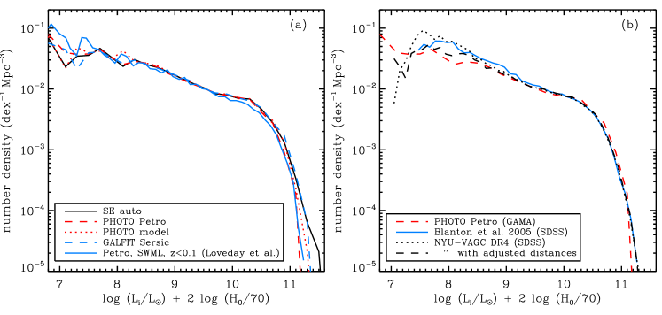
Figure 9: Comparison between $i$-band GLFs. (a): The red lines, black line and blue dashed line represent GLFs computed using the same weights ($1/V^{\prime}_{\rm max}$) but different aperture photometry from SDSS pipeline photo, SExtractor (the Hill et al. 2011 GAMA photometry) and galfit (the Kelvin et al. 2011 Sersic fits). The blue solid line shows the result using the SWML method as per Loveday et al. (2012) applied to a $z<0.1$ sample. (b): The red dashed line is unchanged. The blue line is from the uncorrected (for completeness) GLF of Blanton et al. (2005a), and the black dotted line is computed using the same method and sample from BGD08. The black dashed line is the same sample with the distances adjusted to the Tonry et al. (2000) flow model.

The difference between the GLFs in Fig. 9(a) are generally small except for the SWML $z<0.1$ GLF which is lower around the ‘knee’. The $z<0.1$ GAMA volume is known to be underdense by about 15% with respect to a larger SDSS volume (see fig. 20 of Driver et al. 2011) whereas the $z<0.06$ GAMA density is similar to the SDSS volume. When the SWML method is applied to a $z<0.06$ GAMA sample, there is significantly better agreement with the density-corrected $V^{\prime}_{\rm max}$ LF as expected. Thus the $z<0.1$ LF has a different normalisation and shape primarily because the $i$-band LF is not exactly universal between different environments.

The faint end differences in Fig. 9(a) are generally not significant (cf. error bars in Fig. 8). At the bright end, the differences are because the auto apertures and Sersic fits are recovering more flux from early-type galaxies than the Petrosian aperture.

Figure 9(b) compares the GAMA result using photo Petrosian magnitudes with results using the SDSS NYU-VAGC low-redshift sample ($0.0033<z<0.05$; Blanton et al. 2005b). Ignoring the differences below $10^{7.5}{\rm L}_{\odot}$, which are because of the differing magnitude limits, the Blanton et al. (2005a) GLF (DR2) gives a higher number density below $10^{9}{\rm L}_{\odot}$. This can be at least partly explained by the distances used. The NYU-VAGC uses distances from the Willick et al. (1997) model, tapering to the LG frame beyond 90 Mpc. The black dotted line in Fig. 9(b) represents the $i$-band GLF calculated using the method and sample of BGD08 (DR4) with the NYU-VAGC distances, while for the black dashed line the distances were changed to those derived from the Tonry et al. (2000) model. The latter model gives on average 10%, and up to 30%, larger distances at $z<0.01$. The DR4 result with the adjusted distances is in better agreement with the GAMA result. Note that GAMA galaxies with luminosities $\simeq 10^{8}{\rm L}_{\odot}$ have a median redshift of 0.02 compared to 0.006 for the NYU-VAGC sample. Thus the GAMA result is less sensitive to the flow model at these luminosities. See Loveday et al. (2012) for more details on the GAMA GLFs.

Figure 10 shows the GAMA $i$-band GLF with error bars in comparison with the GLF from a semi-analytical model. The latter was derived by H. Kim & C. Baugh (private communication) using an implementation of galform similar to Bower et al. (2006). The mass resolution of the halo merger trees was improved and the photo-ionisation prescription was changed so that cooling in haloes with a circular velocity below $30{\rm\,km\,s^{-1}}$ (previously $50{\rm\,km\,s^{-1}}$) is prevented after reionisation ($z=6$). There is reasonable agreement between the model and data, however, the model LF is higher particular below $10^{8.2}{\rm L}_{\odot}$. At low luminosities, it is expected that the GAMA data are incomplete because of surface brightness issues and the LF data points are shown as lower limits (justified in the following section, § 3.2).

Figure 10: GAMA data in comparison with a model LF. The model LF was derived by H. Kim & C. Baugh using galform (Bower et al., 2006).

3.2 Surface brightness limit

In addition to the explicit magnitude limit, there is an implicit and imprecisely-defined surface brightness (SB) limit that plagues measurements of the faint end of a GLF (Phillipps & Disney, 1986; Cross & Driver, 2002). Blanton et al. (2005a) estimated the impact on the SDSS GLF, determining a completeness of about 0.7 at $\mu_{r,50}=23.0{\rm\,mag\,arcsec}^{-2}$ where this is the SB within the Petrosian half-light radius. Three sources of incompleteness were considered: photometric incompleteness determined from simulations that put fake galaxies in frames run through photo, tiling incompleteness because some of the SDSS area was targeted on versions of photo where the deblender was not performing optimally, and spectroscopic incompleteness. The tiling incompleteness is not an issue here, the issues associated with the photometric incompleteness may be less severe at the GAMA faint limit because for a given SB the galaxies are smaller, meaning fewer problems with deblender shredding and sky subtraction, and the spectroscopic incompleteness can be mitigated by repeated observations of the same target where necessary.

Figure 11 shows the SB versus stellar mass distribution (with masses from the colour-based M/L relation of Taylor et al. 2011, see § 3.3). It is difficult to determine when the input catalogue becomes incomplete. Judging from the slightly higher mean SB at $10^{8}$–$10^{9}{\rm M}_{\odot}$ in the GAMA sample compared to SDSS, we expect that incompleteness becomes significant for surface brightnesses slightly fainter than the Blanton et al. (2005a) estimate. Recently Geller et al. (2011) analysed a $0.02<z<0.1$ sample from the Smithsonian Hectospec Lensing Survey ($R<20.6$). They determined a linear relation between SB and $M_{R}$ for the blue population. This is shown in Fig. 11 after converting to $H_{0}=70$, assuming $\mu_{r,50}={\rm SB}_{R,50}+0.3$ and M/L${}_{R}=0.5$, which is an average value for a star-forming low-mass galaxy. The average GAMA SB-mass relation falls below this relation at ${\cal M}<10^{8}{\rm M}_{\odot}$, which is where we expect incompleteness to become significant. Rather than attempting to correct for this incompleteness, we assume that the GSMF values below $10^{8}{\rm M}_{\odot}$ are lower limits. For the $i$-band LF, values below $10^{8.2}{\rm L}_{\odot}$ were taken to be lower limits (Fig. 10) because the M/L_i of dwarf galaxies around $10^{8}{\rm M}_{\odot}$ is typically less than 0.8 from the fitting of Taylor et al. (2011).

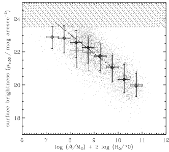
Figure 11: Surface brightness versus stellar mass. The black diamonds and bars represent the GAMA sample used in this paper, while the grey squares and bars show the results from an SDSS $z<0.05$ sample (as per fig. 4 of BGD08). The vertical bars represent the measured scatter, $\pm 1\sigma$, around the median in bins of 0.5 dex. $\mu_{r,50}$ is the SB within the Petrosian half-light radius. The grey dashed-line region represents the expected area of low completeness. The dash-and-dotted line shows the blue population relation converted from Geller et al. (2011).

3.3 Galaxy stellar mass functions

Various authors have suggested that M/L in the $i$-band or $z$-band correlates most usefully with $g-i$ (Gallazzi & Bell 2009; Zibetti, Charlot, & Rix 2009; Taylor et al. 2010b). The parametrization is usually linear as follows

$$\log({\cal M}/L_{i})=a+b(g-i)$$ (5)

where ${\cal M}$ is the stellar mass and $L_{i}$ is the luminosity in solar units. However, estimates of $a$ and $b$ can vary considerably. Bell et al. (2003) give $a=-0.152$ and $b=0.518$ while reading off from figure 4 of Zibetti et al. (2009) gives $a\simeq-1$ and $b\simeq 1$, though the latter is for resolved parts of galaxies. From fitting to the GAMA data, Taylor et al. (2011) obtained $a=-0.68$ and $b=0.73$. This is close to the values obtained from fitting to SDSS colours and the Kauffmann et al. (2003) stellar mass estimates, for example.

Figure 12(a) shows GSMFs from GAMA data testing the effect of varying colour-based M/L_i. The values of $a$ and $b$ are such that the M/L_i is 2.0 for galaxies with $g-i=1.2$. The GSMFs show the flattening around and below $10^{10.5}{\rm M}_{\odot}$, with a steepening below $10^{9.5}{\rm M}_{\odot}$: this is more pronounced with $b=1$ than $b=0.5$. Also shown is a comparison with the results of BGD08. There is generally good agreement between the GAMA and BGD08 results except at $<10^{8.2}{\rm M}_{\odot}$. This is despite the fact that the BGD08 results are expected to be less complete in terms of SB. As noted above, this is because of the distance model used for the redshifts in BGD08. If the distances are changed to the model used here then there is good agreement. The GAMA results are more reliable at $\sim 10^{8}{\rm M}_{\odot}$ because of the minimal dependence on the distance model. For galaxies with $10^{8}<{\cal M}/{\rm M}_{\odot}<10^{8.4}$, 90% are brighter than $M_{r}=-16$, the GLF or GSMF is not significantly affected by uncertainties in the distances (Fig. 3).

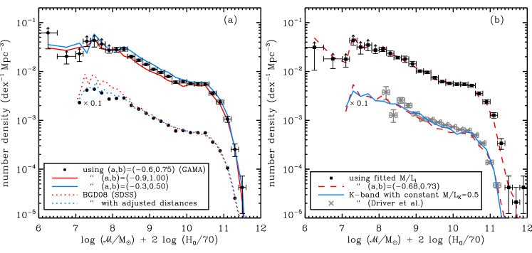
Figure 12: Galaxy stellar mass functions. (a): These GSMFs were derived from Petrosian magnitudes. The symbols with error bars represent the GAMA data using a color-based M/L_i (Eq. 5); the colours were derived from the GAMA auto photometry. The red and blue solid lines were computed using different $a,b$ values. The red and blue dotted lines (offset $\times 0.1$) represent the results from BGD08 and the recomputation using the same sample after changing the flow model to that used here, respectively. (b): The symbols use the fitted GAMA stellar M/L_i from Taylor et al. (2011) applied to the $i$-band Sersic fluxes, while the dotted line uses a color-based M/L_i. The solid line (offset $\times 0.1$) shows effectively the $K$-band GLF with $K=K_{\rm auto}-i_{\rm auto}+i_{\rm Sersic}$ and applying a constant M/L_K, while the crosses with error bars show the Driver et al. (2012) $K$-band GLF.

Figure 12(b) shows the GSMF from the stellar masses of Taylor et al. (2011), strictly the fitted M/L_i ratios in the auto apertures applied to the flux derived from the Sersic $i$-band fit (binned GSMF given in Table 1), and the GSMF derived using the best-fit colour-based M/L_i. These are nearly the same suggesting that a colour-based M/L_i is easily sufficient for determining a GSMF assuming of course that it is calibrated correctly. From the GSMF, the total stellar mass density is $2.3\times 10^{8}{\rm M}_{\odot}{\rm\,Mpc}^{-3}$. This gives an $\Omega_{\rm stars}$ value of 0.0017 (relative to the critical density), or about 4% of the baryon density, which is on the low-end of the range of estimates discussed by BGD08.

Table 1: Galaxy stellar mass function. The $\phi$ values for masses lower than $10^{8}{\rm M}_{\odot}$ should be regarded as lower limits (see § 3.2). The errors quoted are pseudo Poisson errors derived from the square root of the sum of weights squared.

$\log({\cal M}/{\rm M}_{\odot})$	bin	$\phi/10^{-3}$	error	number
mid point	width	${\rm dex^{-1}\,Mpc^{-3}}$
6.25	0.50	31.1	21.6	9
6.75	0.50	18.1	6.6	19
7.10	0.20	17.9	5.7	18
7.30	0.20	43.1	8.7	46
7.50	0.20	31.6	9.0	51
7.70	0.20	34.8	8.4	88
7.90	0.20	27.3	4.2	140
8.10	0.20	28.3	2.8	243
8.30	0.20	23.5	3.0	282
8.50	0.20	19.2	1.2	399
8.70	0.20	18.0	2.6	494
8.90	0.20	14.3	1.7	505
9.10	0.20	10.2	0.6	449
9.30	0.20	9.59	0.55	423
9.50	0.20	7.42	0.41	340
9.70	0.20	6.21	0.37	290
9.90	0.20	5.71	0.35	268
10.10	0.20	5.51	0.34	260
10.30	0.20	5.48	0.34	259
10.50	0.20	5.12	0.33	242
10.70	0.20	3.55	0.27	168
10.90	0.20	2.41	0.23	114
11.10	0.20	1.27	0.16	60
11.30	0.20	0.338	0.085	16
11.50	0.20	0.042	0.030	2
11.70	0.20	0.021	0.021	1
11.90	0.20	0.042	0.030	2

3.4 Comparison with the $K$-band galaxy luminosity function

In order to compare with the shape of the GSMF, we also determined the $K$-band GLF using the same $V^{\prime}_{\rm max}$ values. For this, we used the $K$-band magnitude defined by $K=K_{\rm auto}-i_{\rm auto}+i_{\rm Sersic}$, where the auto photometry is from the $r$-defined catalogue (Hill et al., 2011). The reason for this definition is that for low-SB galaxies an aperture is more accurately defined in the SDSS $r$-band (or $i$-band) compared to the UKIDSS $K$-band. This $K-i$ colour is added to our fiducial $i$-band Sersic magnitude in order to be get a robust estimate of total $K$-band flux. The resulting GLF was simply converted to a GSMF using M/L${}_{K}=0.5$, which was chosen to give approximate agreement with the GSMF derived using the Taylor et al. (2011) stellar masses. The number densities were divided by an average completeness of 0.93 because of the reduced coverage in the $K$-band [fig. 3 of Baldry et al. (2010)]. This scaled GLF is shown by the blue line in Fig. 12(b). Note that strictly the $V^{\prime}_{\rm max}$ values should be recomputed because of the different coverage across the regions but this should have minimal impact on the shape. We also show the GAMA $K$-band GLF from Driver et al. (2012), which was derived from a different sample ($0.013<z<0.1$, $r_{\rm Pet}<19.4$ and $K_{\rm AB}<18.1$ with $r$-defined $K_{\rm auto}$ magnitudes) with the same M/L_K applied.

The flattening from $10^{10.6}{\rm M}_{\odot}$ to $\sim 10^{10}{\rm M}_{\odot}$ and upturn below these masses shown in the $i$-band derived GSMF is also seen directly in the $K$-band GLF [Fig. 12(b)]. Though in the case of the Driver et al. (2012) result (standard $V_{\rm max}$) it is less pronounced. This is an important confirmation of this upturn since, while there is some variation in M/L_K, the $K$-band GLF is often used as a proxy for the GSMF. Previous measurements of the $K$-band field GLF had failed to detect this upturn using 2MASS photometry down to $L_{K}\la 10^{9}{\rm L}_{\odot}$ (Cole et al., 2001; Kochanek et al., 2001) or using UKIDSS with SDSS redshifts (Smith, Loveday, & Cross, 2009); see fig 14. of Smith et al. for a compilation. These measurements nominally probe far enough down the GSMF ($\sim 10^{9}{\rm M}_{\odot}$) that the upturn should have been noted. We note that Merluzzi et al. (2010)’s measurement of the $K$-band GLF in the $z=0.048$ Shapley Cluster shows an upturn particularly in the lower-density environments, however, this does rely on statistical background subtraction. The explanation for 2MASS-based GLFs missing this could be the surface brightness limit. However, GAMA and Smith et al. both used UKIDSS photometry. The difference in this case is that GAMA has redone the near-IR photometry using $r$-band defined matched apertures (Hill et al., 2011), and the magnitude limit is higher meaning the galaxies are typically further away (smaller on the sky) making near-IR photometry more reliable.

3.5 The double Schechter function

The shape of the GSMF is well fit with a double Schechter function with a single value for the break mass (${\cal M}^{*}$), i.e. a five-parameter fit (BGD08; Pozzetti et al. 2010). This is given by

$$\phi_{\cal M}\,{\rm d}{\cal M}=e^{-{\cal M}/{\cal M}^{*}}\left[\phi^{*}_{1}\left(\frac{{\cal M}}{{\cal M}^{*}}\right)^{\alpha_{1}}+\phi^{*}_{2}\left(\frac{{\cal M}}{{\cal M}^{*}}\right)^{\alpha_{2}}\right]\,\frac{{\rm d}{\cal M}}{{\cal M}^{*}}$$ (6)

where $\phi_{\cal M}\,{\rm d}{\cal M}$ is the number density of galaxies with mass between ${\cal M}$ and ${\cal M}+{\rm d}{\cal M}$; with $\alpha_{2}<\alpha_{1}$ so that the second term dominates at the faintest magnitudes. Figure 13 shows this function fitted to the GSMF data providing a good fit. The fit was obtained using a Levenberg-Marquardt algorithm on the binned GSMF between 8.0 and 11.8 (Table 1), and the fit parameters are given in the plot. The fit to the Pozzetti et al. GSMF for $z=0.1$–0.35 is also shown, which is similar.

A natural explanation for this functional form was suggested by Peng et al. (2010b). In their phenomenological model, star-forming (SF) galaxies have a near constant specific star-formation rate (SFR) that is a function of epoch. Then there are two principle processes that turn SF galaxies into red-sequence or passive galaxies: ‘mass quenching’ and ‘environmental quenching’. In the model, the probability of mass quenching is proportional to a galaxy’s SFR (mass times the specific SFR). This naturally produces a (single) Schechter form for the GSMF of SF galaxies. Considering only mass quenching, the GSMF of passive galaxies is also determind to have a Schechter form with the same value of ${\cal M}^{*}$ but with the faint-end (power-law) slope $+1$ compared to that of the SF galaxies. To see this consider a single Schechter function GSMF and multiply by mass: ${\cal M}^{\alpha}\rightarrow{\cal M}^{\alpha+1}$. Overall the GSMF of all galaxies is represented by a double Schechter function with $\alpha_{1}=\alpha_{2}+1$. This is in agreement with our fit (Fig. 13), which has $\alpha_{1}-\alpha_{2}=1.12\pm 0.19$. In fact, a good fit can be obtained by restricting $\alpha_{1}=\alpha_{2}+1$, making a four-parameter fit (at ${\cal M}>10^{8}{\rm M}_{\odot}$).

In the model, environmental quenching does not change the overall double Schechter shape as some SF galaxies are turned to red across all masses. The GSMF of the SF population remains nearly the same shape while the red-sequence GSMF has a scaled ‘copy’ of the SF GSMF added so that it follows a double Schechter form most obviously in high density regions.

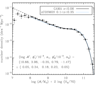
Figure 13: GSMF with a double Schechter fit to data at ${\cal M}>10^{8}{\rm M}_{\odot}$. The data points represent the GAMA fitted stellar mass results. The solid line represents the fit to the data with extrapolation shown by the dashed line. The fit parameters are shown with their 1-sigma errors. Also shown is a fit to zCOSMOS data from Pozzetti et al. (2010).

To illustrate the origin of the double Schechter shape of the GAMA GSMF as suggested by the Peng et al. (2010b) model, we divided the galaxies into red and blue populations based on color-magnitude diagrams. Figure 14 shows the $g-r$ and $u-r$ color-magnitude diagrams both versus $M_{r}$, with three possible dividing lines using a constant slope of $-0.03$ (e.g. Bell et al. 2003) and three using a tanh function (eq. 11 of Baldry et al. 2004), respectively. Figure 15 shows the resulting red- and blue-population GSMFs with the dotted and dashed lines representing the six different colour cuts (some extremely red objects were not included because the colour measurement was unrealistic, $g-r>1.0$ or $u-r>3.2$). Following the Peng et al. (2010b) model, we fit to the red and blue population GSMFs simultaneously with a double Schechter ($\alpha_{1}$, $\alpha_{2}$) and single Schechter function ($\alpha$), respectively. The fits shown in Fig. 15 are constrained to have: the same ${\cal M}^{*}$, $\alpha_{2}=\alpha$, and $\alpha_{1}=\alpha_{2}+1$. A good fit with the five free parameters is obtained to the two populations when using a $u-r$ divider. Note there is an excess of blue population galaxies above a single Schechter fit at high masses when using a $g-r$ divider, the red population data were not fitted below $10^{8.4}{\rm M}_{\odot}$ where there is significant uncertainty in the population type because of presumably large errors in the colours, and the inclusion of edge-on dusty disks is a problem for a simple red colour selection. Nevertheless the basic Peng et al. (2010b) model provides a remarkably simple explanation of the observed GSMF functional forms.

Figure 14: Color-magnitude diagrams. The points represent the GAMA sample used in this paper. The solid and dashed lines represent possible dividing lines between the red and blue populations, with slopes of $-0.03$ in (a) and using a tanh function from Baldry et al. (2004) in (b).

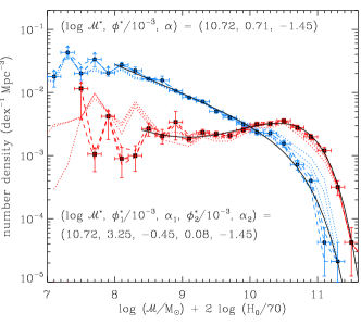
Figure 15: GSMFs for the red and blue populations. The circles and squares with error bars, coloured according to the population, were derived using the divider that is shown as a solid line in Fig. 14(b). The solid lines represent fits to the data. The dotted and dashed lines represent the GSMFs using the six possible dividers based on $g-r$ and $u-r$, respectively.

3.6 The most numerous type of galaxies

Are blue (irregulars, late-type spirals) or red (spheroidals, ellipticals) dwarf galaxies the most numerous type in the Universe (down to $\sim 10^{7}{\rm M}_{\odot}$)? Judging from Fig. 15, the answer would appear to be the blue dwarf galaxies, i.e. star-forming galaxies. However, the measured number densities of both populations may be lower limits; and the measurement of the red population becomes less reliable below about $10^{8.4}{\rm M}_{\odot}$ because of the smaller volume probed, the uncertainties in the colours, and the cosmic variance is larger because the galaxies are more clustered than the blue population.

An alternative estimate of the number densities of red galaxies can be obtained by considering the relative numbers of early-type galaxies in the Local Group, and then scaling the numbers to match the field GSMF at high masses ($>10^{9}{\rm M}_{\odot}$). This assumes that the Local Group represents an average environment in which these galaxies are located. Taking the catalogue of galaxies from Karachentsev et al. (2004), galaxies are selected within 1.4 Mpc and with Galactic extinction less than 1.2 mag. The latter excludes two galaxies viewed near the Galactic plane (a biased direction in terms of detecting the lowest luminosity galaxies). The $B$-band luminosities are converted to stellar masses assuming: M/L_B = 3.0 for early-type galaxies (RC3 type $<0$); M/L_B = 1.0 for M31, M33 and the Milky Way, which have already been corrected for internal attenuation; and M/L_B = 0.5 for late-type galaxies (RC3 type $>6$). From this, there are 6 galaxies with stellar mass $\ga 10^{9}{\rm M}_{\odot}$, which are M31, M32, M33, M110, the Milky Way and LMC. For this population the Local Group, taken to cover a volume of 10 Mpc³, is approximately 50 times higher density than the cosmic average.

Figure 16 shows GSMFs for the field and the Local Group scaled to match, in particular comparing the blue field number densities with that inferred for the early types by scaling. It is likely that the LG sample is complete down to $10^{7}{\rm M}_{\odot}$ with only some recently discovered satellites of M31, e.g. And XXI (Martin et al., 2009), suggesting that the bin shown here from $10^{6}$ to $10^{7}$ is a lower limit. This analysis is consistent with the blue dwarf population being the most common galaxy down to $10^{7}{\rm M}_{\odot}$; at lower masses, it is not yet clear.

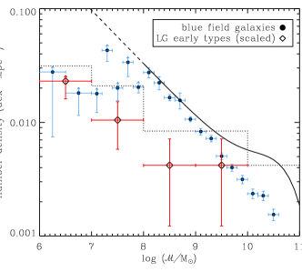
Figure 16: GSMFs for the field (GAMA) and the Local Group (derived from Karachentsev et al. 2004). The solid line shows the GAMA fit from Fig. 13 with the dashed line representing the extrapolation. The dotted line represents the scaled LG GSMF in bins of 1 dex. The circles represent the blue field population while the diamonds represent the LG early types.

3.7 Future work

The GAMA GSMF is reliable down to $10^{8}{\rm M}_{\odot}$ (corresponding to $M_{r}\sim-16$ with M/L${}_{r}=0.5$), which confirms the SDSS result (BGD08) with minor modification to the distances, assuming that the M/L values are approximately correct as a function of a galaxy’s colour. In addition, there are $\sim 350$ galaxies in this GAMA sample between $10^{7}$ and $10^{8}{\rm M}_{\odot}$, and $\sim 30$ between $10^{6}$ and $10^{7}{\rm M}_{\odot}$. There are a number of improvements to be made for the GAMA GSMF measurement at ${\cal M}<10^{8}{\rm M}_{\odot}$:

1. The GAMA survey is ongoing with an aim to complete redshifts to $r<19.8$ over 300 deg². This will approximately treble the volume surveyed for low-luminosity galaxies.

2. There are about 2000 galaxies so far that have been spectroscopically observed twice but with $Q\leq 2$. A careful coadd of the duplicate observations will yield additional redshifts for some of the low-SB galaxies.

3. Flux measurements of currently identified low-mass galaxies can be improved by careful selection of appropriate apertures. Automated Petrosian or Sersic fitting can lead to large errors for well-resolved irregular galaxies.

4. Specialised searches can be made for low-SB galaxies that were missed by SDSS photo, in particular, on deeper imaging provided by the Kilo-Degree Survey (KIDS) with the VLT Survey Telescope and the VISTA Kilo-Degree Infrared Galaxy Survey (VIKING). In the longer term, a space-based half-sky survey, such as that planned for the Euclid mission (Laureijs et al., 2010) of the European Space Agency, potentially will be able to detect low-SB galaxies with $10^{5}<{\cal M}/{\rm M}_{\odot}<10^{6}$ over $10^{5}{\rm\,Mpc^{3}}$.

The expected currently missed detection of low-SB galaxies is critical. In this sample, the observed number density for galaxies with $10^{6.5}$ to $10^{7}{\rm M}_{\odot}$ is only $\sim 0.02\,{\rm Mpc}^{-3}\,{\rm dex}^{-1}$ estimated using the density-corrected $V^{\prime}_{\rm max}$ method. The predicted number by Guo et al. (2011) and by extrapolation of the double Schechter function is $>0.1\,{\rm Mpc}^{-3}\,{\rm dex}^{-1}$. Thus we could be missing significant numbers of larger low-mass galaxies.

Figure 17 shows the observed size-mass relation of galaxies from GAMA for blue and red galaxy populations. For comparison, also shown are measurements of irregular galaxies (Hunter & Elmegreen, 2006) using M/L_V from the $B-V$ relation of Bell et al. (2003), and Milky Way (Gilmore et al., 2007) and M31 dwarf spheroidals (e.g. McConnachie & Irwin 2006; Martin et al. 2009) using M/L${}_{V}=2$. The GAMA relation for the blue population follows an approximately linear relation above $\sim 10^{7.5}{\rm M}_{\odot}$ but appears to drop below the linear extrapolation at lower masses. The dotted line outlines the region where possible low-SB galaxies missed by SDSS selection would be located. These would have $\mu_{r,50}\sim 24$–25 mag arcsec^-2 for the low M/L blue population. This is where an extrapolation of the mass-SB relation to low masses would lie (Fig. 11). Thus it is essential to use a detection algorithm that is sensitive to these types of sources (e.g. Kniazev et al. 2004) at distances $\sim$10–50 Mpc in order to test whether the lowest-mass bins are incomplete within the GAMA survey volume. For the star-forming population, obtaining redshifts is feasible but IFUs would be required if only part of each galaxy has detectable line emission.

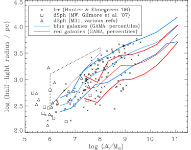
Figure 17: Size-mass relations. The blue and red solid lines show the 16th, median and 84th percentiles of the effective radii from the GAMA Sersic fits (Kelvin et al., 2011) for the blue and red populations. The symbols represent measurements for irregulars and dwarf spheroidals. The dotted line outlines the region of incompleteness because of SB limits relating to the current GAMA sample.

The low-redshift sample here only uses 5 per cent of the GAMA $r$-band limited main survey. The GAMA survey is also well placed to measure the evolution of the GSMF out to $z\sim 0.6$ for the most massive galaxies, study variations with environment and halo mass, and to study variations in properties with stellar mass.

4 Summary and conclusions

We present an investigation of the GSMF using the GAMA survey. Throughout the paper, a recurring theme has been the ways in which different aspects of the analysis can affect the inferred shape and normalisation of a GLF or GSMF. In particular we have explored the importance of accounting for: bulk flows when estimating distances, large scale structure when estimating effective maximum volumes, the effect of using different photometric measures, the surface brightness limit, and the effect of using different simple prescriptions to estimate stellar mass.

The distance moduli to apply to the magnitudes depend significantly on using the Tonry et al. (2000) flow model in comparison with fixed frames (Figs. 1–2). There is a noticeable effect on the measured number density of galaxies fainter than $M_{r}=-16$ (Fig. 3). Using the same flow model with SDSS data brings into better agreement measurements of the GLF and GSMF between SDSS and GAMA [Fig. 9(b), Fig. 12(a)]. For the same luminosity galaxies, the $r<19.4$ (19.8 in G12) GAMA sample is less sensitive to whether the flow model is correct than the $r<17.8$ SDSS sample.

Measuring the GSMF accurately over a large mass range requires surveying a suitable volume $\ga 10^{5}{\rm\,Mpc}^{-3}$ to obtain at least tens of galaxies at the high-mass end ($\ga 10^{11}{\rm M}_{\odot}$), while the volume over which low-mass galaxies are observed need not be so large. A problem arises in that the volume over which a galaxy is visible depends on its luminosity, and any variations in density as a function of redshift will distort the shape of a GSMF based on the standard $V_{\rm max}$ method. Here we use a density-corrected $V^{\prime}_{\rm max}$ method. This has been shown to be equivalent to a maximum-likelihood method (Cole, 2011) but is simpler to apply to an estimate of the GSMF. A volume-limited DDP sample of $M_{r}<-17.9$ (Fig. 4) was used to measure relative densities up to a given redshift (Fig. 6); and these are used to produce the density-corrected volumes (Eq. 4). A useful diagnostic is to plot $V^{\prime}_{\rm max}$ versus $M_{r}$ (Fig. 7), which shows that $V^{\prime}_{\rm max}$ increases nearly monotonically but with changes in slope compared to $V_{\rm max}$. The density-corrected $V^{\prime}_{\rm max}$ method significantly reduces the difference in the measured GLFs between the regions compared to using the standard $V_{\rm max}$ method (Fig. 8).

There are small differences in the measured $i$-band GLF depending on the method of determining a galaxy’s flux [Fig. 9(a)]. The auto apertures and Sersic fits recover more flux from early-type galaxies than the Petrosian aperture. This makes a significant difference at the bright end of the GLF. Converting the GLF to a GSMF using a colour-based M/L_i relation results in a more obvious flattening and rise from high to low masses as the $b$ parameter is increased [Fig. 12(a)]. Similar GSMF results are obtained whether using a fitted M/L_i for each galaxy or the colour-based M/L_i from Taylor et al. (2011) [Fig. 12(b)]. This is not surprising because the GSMF is only a one-dimensional distribution. We also find that the $K$-band produces a similar GSMF using a constant M/L${}_{K}=0.5$. This is an important verification of the upturn based on a simpler assumption that the $K$-band approximately traces the stellar mass.

As in BGD08 and Pozzetti et al. (2010), we find that the double Schechter function provides a good fit to the data for ${\cal M}>10^{8}{\rm M}_{\odot}$ (Fig. 13). This is approximately the sum of a single Schechter function for the blue population and double Schechter function for the red population (Fig. 15). This supports the empirical picture, quenching model, for the origin of the Schechter function by Peng et al. (2010b).

Blind redshift surveys, like GAMA, are better at characterising the GSMF for the star-forming field population than the fainter and more clustered red population. In order to test whether the blue population is the most numerous in the mass range $10^{7}-10^{8}{\rm M}_{\odot}$ as implied by the GAMA GSMF, we determined an approximate LG GSMF and scaled the resulting numbers to match the field GSMF at masses $>10^{9}{\rm M}_{\odot}$ (Fig. 16). The numbers of early types in the cosmic-average GSMF implied by this analysis are below that of the directly measured blue population.

Accurately measuring the GSMF below $10^{8}{\rm M}_{\odot}$ is key to probing new physics. For example, a simple prescription for preventing star formation in low-mass haloes, considering temperature-dependent accretion and supernovae feedback, results in a peak in the GSMF for star-forming galaxies at about $10^{7}{\rm M}_{\odot}$ (Mamon et al., 2011) (note the overall baryonic mass function continues to rise in their model). The problem with observing low-mass galaxies, $10^{6}$–$10^{8}{\rm M}_{\odot}$, is not the GAMA spectroscopic survey limit ($r<19.8$) at least for the star-forming population but primarily the well-known issue with detecting low-SB galaxies (Fig. 11). Thus a future aim for the GAMA survey is to characterise the extent of the missing $\sim{\rm kpc}$ size low-mass population (Fig. 17), which ultimately will require high quality deep imaging with specialised followup.

References

- Adelman-McCarthy et al. (2008) Adelman-McCarthy J. K., et al., 2008, ApJS, 175, 297
- Avni & Bahcall (1980) Avni Y., Bahcall J. N., 1980, ApJ, 235, 694
- Baldry et al. (2006) Baldry I. K., Balogh M. L., Bower R. G., Glazebrook K., Nichol R. C., Bamford S. P., Budavari T., 2006, MNRAS, 373, 469
- Baldry et al. (2004) Baldry I. K., Glazebrook K., Brinkmann J., Ivezić Ž., Lupton R. H., Nichol R. C., Szalay A. S., 2004, ApJ, 600, 681
- Baldry et al. (2008) Baldry I. K., Glazebrook K., Driver S. P., 2008, MNRAS, 388, 945
- Baldry et al. (2010) Baldry I. K., et al., 2010, MNRAS, 404, 86
- Balogh et al. (2001) Balogh M. L., Christlein D., Zabludoff A. I., Zaritsky D., 2001, ApJ, 557, 117
- Bell & de Jong (2001) Bell E. F., de Jong R. S., 2001, ApJ, 550, 212
- Bell et al. (2003) Bell E. F., McIntosh D. H., Katz N., Weinberg M. D., 2003, ApJS, 149, 289
- Benson et al. (2002) Benson A. J., Lacey C. G., Baugh C. M., Cole S., Frenk C. S., 2002, MNRAS, 333, 156
- Bertin & Arnouts (1996) Bertin E., Arnouts S., 1996, A&AS, 117, 393
- Best et al. (2005) Best P. N., Kauffmann G., Heckman T. M., Brinchmann J., Charlot S., Ivezić Ž., White S. D. M., 2005, MNRAS, 362, 25
- Binggeli et al. (1988) Binggeli B., Sandage A., Tammann G. A., 1988, ARA&A, 26, 509
- Blanton et al. (2005a) Blanton M. R., Lupton R. H., Schlegel D. J., Strauss M. A., Brinkmann J., Fukugita M., Loveday J., 2005a, ApJ, 631, 208
- Blanton & Roweis (2007) Blanton M. R., Roweis S., 2007, AJ, 133, 734
- Blanton et al. (2003a) Blanton M. R., et al., 2003a, AJ, 125, 2348
- Blanton et al. (2003b) Blanton M. R., et al., 2003b, ApJ, 592, 819
- Blanton et al. (2005b) Blanton M. R., et al., 2005b, AJ, 129, 2562
- Bower et al. (2006) Bower R. G., Benson A. J., Malbon R., Helly J. C., Frenk C. S., Baugh C. M., Cole S., Lacey C. G., 2006, MNRAS, 370, 645
- Boylan-Kolchin et al. (2009) Boylan-Kolchin M., Springel V., White S. D. M., Jenkins A., Lemson G., 2009, MNRAS, 398, 1150
- Brough et al. (2011) Brough S., et al., 2011, MNRAS, 413, 1236
- Brown et al. (2001) Brown W. R., Geller M. J., Fabricant D. G., Kurtz M. J., 2001, AJ, 122, 714
- Bruzual & Charlot (2003) Bruzual G., Charlot S., 2003, MNRAS, 344, 1000
- Calzetti et al. (2000) Calzetti D., Armus L., Bohlin R. C., Kinney A. L., Koornneef J., Storchi-Bergmann T., 2000, ApJ, 533, 682
- Caputi et al. (2011) Caputi K. I., Cirasuolo M., Dunlop J. S., McLure R. J., Farrah D., Almaini O., 2011, MNRAS, 413, 162
- Chabrier (2003) Chabrier G., 2003, PASP, 115, 763
- Chiboucas et al. (2009) Chiboucas K., Karachentsev I. D., Tully R. B., 2009, AJ, 137, 3009
- Cole (2011) Cole S., 2011, MNRAS, 416, 739
- Cole et al. (2001) Cole S., et al., 2001, MNRAS, 326, 255
- Conroy et al. (2009) Conroy C., Gunn J. E., White M., 2009, ApJ, 699, 486
- Conroy & Wechsler (2009) Conroy C., Wechsler R. H., 2009, ApJ, 696, 620
- Courteau & van den Bergh (1999) Courteau S., van den Bergh S., 1999, AJ, 118, 337
- Croom et al. (2004) Croom S., Saunders W., Heald R., 2004, Anglo-Australian Obser. Newsletter, 106, 12
- Cross & Driver (2002) Cross N., Driver S. P., 2002, MNRAS, 329, 579
- Croton et al. (2006) Croton D. J., et al., 2006, MNRAS, 365, 11
- Davé (2008) Davé R., 2008, MNRAS, 385, 147
- Dekel & Birnboim (2006) Dekel A., Birnboim Y., 2006, MNRAS, 368, 2
- Dekel & Silk (1986) Dekel A., Silk J., 1986, ApJ, 303, 39
- Dickinson et al. (2003) Dickinson M., Papovich C., Ferguson H. C., Budavári T., 2003, ApJ, 587, 25
- Driver et al. (2007) Driver S. P., Popescu C. C., Tuffs R. J., Liske J., Graham A. W., Allen P. D., de Propris R., 2007, MNRAS, 379, 1022
- Driver et al. (2009) Driver S. P., et al., 2009, Astron. Geophys., 50, 5.12
- Driver et al. (2011) Driver S. P., et al., 2011, MNRAS, 413, 971
- Driver et al. (2012) Driver S. P., et al., 2012, MNRAS, submitted
- Drory et al. (2009) Drory N., et al., 2009, ApJ, 707, 1595
- Efstathiou (1992) Efstathiou G., 1992, MNRAS, 256, 43P
- Efstathiou et al. (1988) Efstathiou G., Ellis R. S., Peterson B. A., 1988, MNRAS, 232, 431
- Elsner et al. (2008) Elsner F., Feulner G., Hopp U., 2008, A&A, 477, 503
- Erdoğdu et al. (2006) Erdoğdu P., et al., 2006, MNRAS, 368, 1515
- Felten (1977) Felten J. E., 1977, AJ, 82, 861
- Gallazzi & Bell (2009) Gallazzi A., Bell E. F., 2009, ApJS, 185, 253
- Gallazzi et al. (2005) Gallazzi A., Charlot S., Brinchmann J., White S. D. M., Tremonti C. A., 2005, MNRAS, 362, 41
- Geller et al. (2011) Geller M. J., Diaferio A., Kurtz M. J., Dell’Antonio I. P., Fabricant D. G., 2011, AJ, submitted (arXiv:1107.2930)
- Gilbank et al. (2011) Gilbank D. G., et al., 2011, MNRAS, 414, 304
- Gilmore et al. (2007) Gilmore G., Wilkinson M. I., Wyse R. F. G., Kleyna J. T., Koch A., Evans N. W., Grebel E. K., 2007, ApJ, 663, 948
- González et al. (2011) González V., Labbé I., Bouwens R. J., Illingworth G., Franx M., Kriek M., 2011, ApJ, 735, L34
- Guo et al. (2010) Guo Q., White S., Li C., Boylan-Kolchin M., 2010, MNRAS, 404, 1111
- Guo et al. (2011) Guo Q., et al., 2011, MNRAS, 413, 101
- Hill et al. (2010) Hill D. T., Driver S. P., Cameron E., Cross N., Liske J., Robotham A., 2010, MNRAS, 404, 1215
- Hill et al. (2011) Hill D. T., et al., 2011, MNRAS, 412, 765
- Hunter & Elmegreen (2006) Hunter D. A., Elmegreen B. G., 2006, ApJS, 162, 49
- Jablonka & Arimoto (1992) Jablonka J., Arimoto N., 1992, A&A, 255, 63
- Jones et al. (2006) Jones D. H., Peterson B. A., Colless M., Saunders W., 2006, MNRAS, 369, 25
- Kajisawa et al. (2009) Kajisawa M., et al., 2009, ApJ, 702, 1393
- Karachentsev et al. (2004) Karachentsev I. D., Karachentseva V. E., Huchtmeier W. K., Makarov D. I., 2004, AJ, 127, 2031
- Kauffmann et al. (2003) Kauffmann G., et al., 2003, MNRAS, 341, 33
- Kay et al. (2002) Kay S. T., Pearce F. R., Frenk C. S., Jenkins A., 2002, MNRAS, 330, 113
- Kelvin et al. (2011) Kelvin L., et al., 2011, MNRAS, in press (arXiv:1112.1956)
- Kereš et al. (2005) Kereš D., Katz N., Weinberg D. H., Davé R., 2005, MNRAS, 363, 2
- Kniazev et al. (2004) Kniazev A. Y., Grebel E. K., Pustilnik S. A., Pramskij A. G., Kniazeva T. F., Prada F., Harbeck D., 2004, AJ, 127, 704
- Kochanek et al. (2001) Kochanek C. S., et al., 2001, ApJ, 560, 566
- Koposov et al. (2008) Koposov S., et al., 2008, ApJ, 686, 279
- Kroupa (2001) Kroupa P., 2001, MNRAS, 322, 231
- Lacey & Silk (1991) Lacey C., Silk J., 1991, ApJ, 381, 14
- Larson (1974) Larson R. B., 1974, MNRAS, 169, 229
- Larson & Tinsley (1978) Larson R. B., Tinsley B. M., 1978, ApJ, 219, 46
- Laureijs et al. (2010) Laureijs R. J., Duvet L., Escudero Sanz I., Gondoin P., Lumb D. H., Oosterbroek T., Saavedra Criado G., 2010, Proc. SPIE, 7731, 77311H
- Lawrence et al. (2007) Lawrence A., et al., 2007, MNRAS, 379, 1599
- Li & White (2009) Li C., White S. D. M., 2009, MNRAS, 398, 2177
- Lineweaver et al. (1996) Lineweaver C. H., Tenorio L., Smoot G. F., Keegstra P., Banday A. J., Lubin P., 1996, ApJ, 470, 38
- Loveday et al. (1992) Loveday J., Peterson B. A., Efstathiou G., Maddox S. J., 1992, ApJ, 390, 338
- Loveday et al. (2012) Loveday J., et al., 2012, MNRAS, 420, 1239
- Mahtessian (2011) Mahtessian A. P., 2011, Astrophysics, 54, 162
- Mamon et al. (2011) Mamon G. A., Tweed D., Cattaneo A., Thuan T. X., 2011, in EAS Publ. Ser., Vol. 48, A Universe of Dwarf Galaxies., M. Koleva, P. Prugniel, & I. Vauglin, ed., p. 435
- Maraston et al. (2006) Maraston C., Daddi E., Renzini A., Cimatti A., Dickinson M., Papovich C., Pasquali A., Pirzkal N., 2006, ApJ, 652, 85
- Marchesini et al. (2009) Marchesini D., van Dokkum P. G., Förster Schreiber N. M., Franx M., Labbé I., Wuyts S., 2009, ApJ, 701, 1765
- Marinoni & Hudson (2002) Marinoni C., Hudson M. J., 2002, ApJ, 569, 101
- Martin et al. (2009) Martin N. F., et al., 2009, ApJ, 705, 758
- Masters et al. (2004) Masters K. L., Haynes M. P., Giovanelli R., 2004, ApJ, 607, L115
- McConnachie & Irwin (2006) McConnachie A. W., Irwin M. J., 2006, MNRAS, 365, 1263
- Mercurio et al. (2006) Mercurio A., et al., 2006, MNRAS, 368, 109
- Merluzzi et al. (2010) Merluzzi P., Mercurio A., Haines C. P., Smith R. J., Busarello G., Lucey J. R., 2010, MNRAS, 402, 753
- Mortlock et al. (2011) Mortlock A., Conselice C. J., Bluck A. F. L., Bauer A. E., Grützbauch R., Buitrago F., Ownsworth J., 2011, MNRAS, 413, 2845
- Moster et al. (2010) Moster B. P., Somerville R. S., Maulbetsch C., van den Bosch F. C., Macciò A. V., Naab T., Oser L., 2010, ApJ, 710, 903
- Norberg et al. (2002) Norberg P., et al., 2002, MNRAS, 336, 907
- Oppenheimer et al. (2010) Oppenheimer B. D., Davé R., Kereš D., Fardal M., Katz N., Kollmeier J. A., Weinberg D. H., 2010, MNRAS, 406, 2325
- Panter et al. (2004) Panter B., Heavens A. F., Jimenez R., 2004, MNRAS, 355, 764
- Panter et al. (2007) Panter B., Jimenez R., Heavens A. F., Charlot S., 2007, MNRAS, 378, 1550
- Peng et al. (2010a) Peng C. Y., Ho L. C., Impey C. D., Rix H.-W., 2010a, AJ, 139, 2097
- Peng et al. (2010b) Peng Y., et al., 2010b, ApJ, 721, 193
- Phillipps & Disney (1986) Phillipps S., Disney M., 1986, MNRAS, 221, 1039
- Popescu et al. (2000) Popescu C. C., Misiriotis A., Kylafis N. D., Tuffs R. J., Fischera J., 2000, A&A, 362, 138
- Pozzetti et al. (2010) Pozzetti L., et al., 2010, A&A, 523, A13
- Rines & Geller (2008) Rines K., Geller M. J., 2008, AJ, 135, 1837
- Robotham et al. (2010) Robotham A., et al., 2010, Publ. Astron. Soc. Australia, 27, 76
- Sabatini et al. (2003) Sabatini S., Davies J., Scaramella R., Smith R., Baes M., Linder S. M., Roberts S., Testa V., 2003, MNRAS, 341, 981
- Salucci & Persic (1999) Salucci P., Persic M., 1999, MNRAS, 309, 923
- Saunders et al. (2004) Saunders W., Cannon R., Sutherland W., 2004, Anglo-Australian Obser. Newsletter, 106, 16
- Saunders et al. (1990) Saunders W., Rowan-Robinson M., Lawrence A., Efstathiou G., Kaiser N., Ellis R. S., Frenk C. S., 1990, MNRAS, 242, 318
- Schechter (1976) Schechter P., 1976, ApJ, 203, 297
- Schlegel et al. (1998) Schlegel D. J., Finkbeiner D. P., Davis M., 1998, ApJ, 500, 525
- Schmidt (1968) Schmidt M., 1968, ApJ, 151, 393
- Shankar et al. (2006) Shankar F., Lapi A., Salucci P., De Zotti G., Danese L., 2006, ApJ, 643, 14
- Sharp et al. (2006) Sharp R., et al., 2006, Proc. SPIE, 6269, 62690G
- Smith et al. (2009) Smith A. J., Loveday J., Cross N. J. G., 2009, MNRAS, 397, 868
- Somerville (2002) Somerville R. S., 2002, ApJ, 572, L23
- Springel et al. (2005) Springel V., et al., 2005, Nature, 435, 629
- Stoughton et al. (2002) Stoughton C., et al., 2002, AJ, 123, 485
- Taylor et al. (2010a) Taylor E. N., Franx M., Brinchmann J., van der Wel A., van Dokkum P. G., 2010a, ApJ, 722, 1
- Taylor et al. (2010b) Taylor E. N., Franx M., Glazebrook K., Brinchmann J., van der Wel A., van Dokkum P. G., 2010b, ApJ, 720, 723
- Taylor et al. (2011) Taylor E. N., et al., 2011, MNRAS, 418, 1587
- Thoul & Weinberg (1996) Thoul A. A., Weinberg D. H., 1996, ApJ, 465, 608
- Tonry et al. (2000) Tonry J. L., Blakeslee J. P., Ajhar E. A., Dressler A., 2000, ApJ, 530, 625
- Trentham & Tully (2002) Trentham N., Tully R. B., 2002, MNRAS, 335, 712
- Tuffs et al. (2004) Tuffs R. J., Popescu C. C., Völk H. J., Kylafis N. D., Dopita M. A., 2004, A&A, 419, 821
- van Dokkum (2008) van Dokkum P. G., 2008, ApJ, 674, 29
- Vulcani et al. (2011) Vulcani B., et al., 2011, MNRAS, 412, 246
- Wake et al. (2006) Wake D. A., et al., 2006, MNRAS, 372, 537
- Watkins et al. (2009) Watkins R., Feldman H. A., Hudson M. J., 2009, MNRAS, 392, 743
- Wilkins et al. (2008) Wilkins S. M., Hopkins A. M., Trentham N., Tojeiro R., 2008, MNRAS, 391, 363
- Willick et al. (1997) Willick J. A., Strauss M. A., Dekel A., Kolatt T., 1997, ApJ, 486, 629
- Zibetti et al. (2009) Zibetti S., Charlot S., Rix H., 2009, MNRAS, 400, 1181