Energy levels of triangular and hexagonal graphene quantum dots: a comparative study between the tight-binding and the Dirac equation approach

Abstract

The Dirac equation is solved for triangular and hexagonal graphene quantum dots for different boundary conditions in the presence of a perpendicular magnetic field. We analyze the influence of the dot size and its geometry on their energy spectrum. A comparison between the results obtained for graphene dots with zigzag and armchair edges, as well as for infinite-mass boundary condition, is presented and our results show that the type of graphene dot edge and the choice of the appropriate boundary conditions have a very important influence on the energy spectrum. The single particle energy levels are calculated as function of an external perpendicular magnetic field which lifts degeneracies. Comparing the energy spectra obtained from the tight-binding approximation to those obtained from the continuum Dirac equation approach, we verify that the behavior of the energies as function of the dot size or the applied magnetic field are qualitatively similar, but in some cases quantitative differences can exist.

I Introduction

Since its recent discovery novo1 , graphene (a single layer of carbon atoms) has been attracting a lot of interest, due to its unique band structure, which is gapless and exhibits an approximately linear dispersion relation at two inequivalent points of the reciprocal space (labeled as $K$ and $K^{\prime}$) in the vicinity of the Fermi energy. The linearity of the band structure allows one to describe the carriers close to the $K$ and $K^{\prime}$ points in a continuum model, using the Dirac equation with massless particlesCastroNeto . Because of the well known Klein tunneling effect in graphene, which prevents electrical confinement of electrons, the lateral confinement of Dirac carriers is a big challenge in manufacturing graphene-based electronic devicesKatsnelson ; Milton ; Matulis . Different suggestions have been made to realize lateral confinement of electrons in graphene, e.g. by means of gap engineering, provided by a space dependent mass term, GiavarasNori1 ; GiavarasNori2 or, alternatively, by combining an external magnetic field Giavaras or a finite mass term Recher with an electrostatic potential. On the other hand, recent improvements of different fabrication techniques made possible cutting and manufacturing of single layer graphene flakes, with different shapes and sizesNovoselov3 ; Hiura ; Subramanian , where such a lateral confinement naturally occurs. Using the tight-binding model (TBM), remarkable effects have been reported as a consequence of the type of the edges and the geometry of these flakesEzawa ; Guclu ; Heiskanen ; Akola ; Zhang ; Kosimov ; Ligia2 : i) zero-energy states are predicted for triangular graphene flakes with zigzag boundaries, ii) for very small flakes a gap opens (the energy gap of different graphene flakes was recently investigated experimentallyritter ) and the density of states (DOS) strongly depends on the type of the edges for any dot geometry, and iii) the energy levels of graphene quantum dots in the presence of a magnetic field approach the Landau levels with increasing magnetic field.

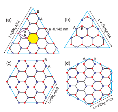
Figure 1: (Color online) The lattice structure of triangular (upper panels) and hexagonal (lower panels) graphene quantum dots with (a,c) armchair edges and (b,d) zigzag edges. $a=0.142$ nm is the C-C distance and the primitive lattice vectors are denoted by a and b. The atoms of the two sublattices are represented by blue circles and red dots. The yellow region indicates the area of one carbon hexagon. $N_{s}$ is the number of C-atoms in each side of the dot.

Recently, analytical results were reported for infinite mass boundary conditions for circular disks, Schnez for triangular flakes with armchair edgesRozhkov and zigzag edgesGuclu and for square graphene quantum dotsTang . However, it is not always clear how the complicated boundary conditions describing the zigzag and armchair edges can be invoked in the continuum model. Furthermore, the geometry of the triangular and hexagonal graphene flakes, make such systems harder to be studied by analytical means. One has to rely on, either a tight-binding model or a numerical solution of coupled differential equations in case of the continuum model.

The continuum model describes very well the low energy states in an infinite graphene sheet, but it is not clear if this is still the case for small graphene flakes. Therefore, it is important to learn if there is a minimum size beyond which the continuum model no longer gives reliable predictions. Furthermore, because of the large influence of the type of edges on the energy spectrum, and since it is not always clear which boundary conditions should be invoked in the Dirac equation for each possible geometry of the flake, a comparison between the results obtained with the different possible boundary conditions and a link with the TBM is an interesting issue which requires a detailed study.

In this paper, by solving the Dirac equation numerically, we present a theoretical study of the energy spectra of triangular and hexagonal graphene quantum dots, where three types of boundary conditions are invoked, namely, zigzag, armchair and infinite mass boundary condition. The influence of an external magnetic field, perpendicular to the graphene layer, on the energy spectrum of the quantum dots is also analyzed. A comparison between the results obtained with the continuum model and those obtained from the tight-binding approach will be made.

This paper is organized as follows. In Sec. II we present a brief outline of the tight-binding model (TBM). The model based on the Dirac-Weyl equation is presented in Sec. III and the different boundary conditions are separately analyzed in this section. Our numerical results are reported in Sec. IV. The summary and conclusions of this work are presented in Sec. V.

II Tight-binding model

The tight-binding Hamiltonian within the nearest neighbor approximation is

$$H=\sum_{n}E_{n}c_{n}c_{n}^{{\dagger}}+\sum_{<n,m>}(t_{n,m}c_{n}^{{\dagger}}c_{m}+h.c.),$$ (1)

where $E_{n}$ is the energy of the $n$-th site, $t_{n,m}$ is the hopping energy and $c_{n}^{{\dagger}}$ ($c_{n}$) is the creation (annihilation) operator of the $\pi$ electron at site $n$. Note that, for each site $n$, the summation is taken over all nearest neighboring sites $m$. In the presence of a magnetic field, the transfer energy becomes $\displaystyle{t\rightarrow te^{i2\pi\Phi_{n,m}}}$, where $\Phi_{n,m}=(1/\Phi_{0})\int_{r_{n}}^{r_{m}}\mathbf{A}\cdot\mathbf{dl}$ is the Peierls phase, with $\Phi_{0}=h/e$ the magnetic quantum flux and $\mathbf{A}$ the vector potential.

Triangular and hexagonal quantum dots with zigzag and armchair edges are illustrated in Fig. 1, where the vectors $\mathbf{a}=a(3/2,\sqrt{3}/2)$ and $\mathbf{b}=a(3/2,-\sqrt{3}/2)$, with $a=0.142$ nm the lattice parameter (or the C-C distance), are introduced as primitive lattice vectors. In the present work, we will consider only the interaction between each atom $n$ and its three first nearest neighbors. In the case of graphene, this interaction has the hopping energy $t=2.7$ eV. The vector potential corresponding to the external magnetic field $\mathbf{B}=B\hat{z}$ perpendicular to the layer is chosen as the Landau gauge $A=(0,Bx,0)$. With this choice of gauge, the Peierls phase for a transition between two sites $n$ and $m$ is $\Phi_{n,m}=0$ in the $x$ direction and $\Phi_{n,m}=\pm(x/3a)\Phi_{c}/\Phi_{0}$ along the $\pm y$ direction, where $\Phi_{c}=3\sqrt{3}a^{2}B/2$ is the magnetic flux threading one carbon hexagon (the area of one carbon hexagon is shown in Fig. 1(a) by the yellow region). An external potential is represented by a variation in the on-site energies $E_{n}$, and a vacancy or defect can be represented by setting the energy of the vacant site to a larger value and the hopping terms to these atoms as zero Ligia . The Hamiltonian $H$ in Eq. (1) can be represented in matrix form and the eigenvalues and eigenfunctions of a graphene flake can be obtained by diagonalization of the matrix.

Notice that the hexagonal lattice presented in Fig. 1 is not a Bravais lattice, but a combination of two triangular lattices composed by atoms labeled as type A (blue) and type B (red). Accordingly, the tight-binding Hamiltonian of Eq. (1) can be rewritten as

$$H=\sum_{n}E_{n}^{A}a_{n}^{{\dagger}}a_{n}+\sum_{n}E_{n}^{B}b_{n}^{{\dagger}}b_{n}+\sum_{<n,m>}(t_{n,m}a_{n}^{{\dagger}}b_{m}+h.c.)$$ (2)

where the operators $a_{n}^{{\dagger}}$ ($a_{n}$) and $b_{n}^{{\dagger}}$ ($b_{n}$) create (annihilate) an electron in site $n$ of lattice A and B, respectively.

III Continuum model: Dirac-Weyl equation

Considering an infinite (periodic) graphene sheet and after, performing a Fourier transform on the operators in Eq. (1) and diagonalizing the resulting Hamiltonian leads to an energy dispersion CastroNeto

$$E(\mathbf{k})=\pm t\sqrt{3+2\cos(\sqrt{3}k_{y}a)+4\cos\left(\frac{\sqrt{3}a}{2}k_{y}\right)\cos\left(\frac{3a}{2}k_{x}\right)}.$$ (3)

The first Brillouin zone in reciprocal space is a hexagon with six Dirac points, where only two of them are inequivalent. From the primitive vectors, we can find the position of these as $\displaystyle{K=(2\pi/3a,2\pi/3\sqrt{3}a)}$ and $\displaystyle{K^{\prime}=(2\pi/3a,-2\pi/3\sqrt{3}a)}$. The states near these points have approximately a linear dispersion and can be described as massless Dirac fermions by the Hamiltonian

$$H=\left(\begin{array}[]{cc}H_{K}&\mathbf{0}\\ \mathbf{0}&H_{K^{\prime}}\\ \end{array}\right),$$ (4)

where $H_{K}$ ($H_{K^{\prime}}$) is the Hamiltonian in the $K$ ($K^{\prime}$) point, which are given by

$$H_{K}=v_{F}~{}\boldsymbol{\sigma}.~{}\mathbf{p},$$ (5a)

$$H_{K^{\prime}}=v_{F}~{}\boldsymbol{\sigma^{\ast}}.~{}\mathbf{p},$$ (5b)

where $\boldsymbol{\sigma}=(\sigma_{x},\sigma_{y})$ are Pauli matrices and $\boldsymbol{\sigma^{\ast}}=(\sigma_{x},-\sigma_{y})$ denotes the complex conjugate of the matrix $\boldsymbol{\sigma}$. In the presence of a magnetic field $B$ perpendicular to the graphene layer and using the Landau gauge, one can simply rewrite Eq. (4) in the following form:

$$H=\left(\begin{array}[]{cccc}0&\Pi_{-}&0&0\\ \Pi_{+}&0&0&0\\ 0&0&0&\Pi_{+}\\ 0&0&\Pi_{-}&0\\ \end{array}\right),$$ (6)

where,

$$\Pi_{\pm}=-i\hbar v_{F}\left[\frac{\partial}{\partial x}\pm i\frac{\partial}{\partial y}\mp\frac{2\pi B}{\Phi_{0}}x\right].$$ (7)

The wave function in real space for the sublattice A is

$$\psi_{A}(\mathbf{r})=e^{i\mathbf{K}\cdot\mathbf{r}}\varphi_{A}(r)+e^{i\mathbf{K^{\prime}}\cdot\mathbf{r}}\varphi_{A^{\prime}}(r),$$ (8a)

and for sublattice B it is given by,

$$\psi_{B}(\mathbf{r})=e^{i\mathbf{K}\cdot\mathbf{r}}\varphi_{B}(r)+e^{i\mathbf{K^{\prime}}\cdot\mathbf{r}}\varphi_{B^{\prime}}(r).$$ (8b)

The Hamiltonian of Eq. (6) acts on the four-component wave function $\Psi=[\varphi_{A},\varphi_{B},\varphi_{A^{\prime}},\varphi_{B^{\prime}}]^{T}$, which leads to the four coupled first-order differential equations:

$$-i\left[\frac{\partial}{\partial x^{\prime}}-i\frac{\partial}{\partial y^{\prime}}+\beta x^{\prime}\right]\varphi_{B}=\epsilon\varphi_{A},$$ (9a)

$$-i\left[\frac{\partial}{\partial x^{\prime}}+i\frac{\partial}{\partial y^{\prime}}-\beta x^{\prime}\right]\varphi_{A}=\epsilon\varphi_{B},$$ (9b)

$$-i\left[\frac{\partial}{\partial x^{\prime}}+i\frac{\partial}{\partial y^{\prime}}-\beta x^{\prime}\right]\varphi_{B^{\prime}}=\epsilon\varphi_{A^{\prime}},$$ (9c)

$$-i\left[\frac{\partial}{\partial x^{\prime}}-i\frac{\partial}{\partial y^{\prime}}+\beta x^{\prime}\right]\varphi_{A^{\prime}}=\epsilon\varphi_{B^{\prime}}.$$ (9d)

In the above equations, we used the following dimensionless units: $x^{\prime}=x/\sqrt{S}$, $y^{\prime}=y/\sqrt{S}$, $\beta=2\pi BS/\Phi_{0}=2\pi\Phi/\Phi_{0}$, $\epsilon=E/E_{0}$, with $E_{0}=\hbar v_{F}/\sqrt{S}$, where $S\propto L^{2}$ is the area of the dot with $L$ being the length of the side of the dot. In this paper, we solve Eqs. (9) numerically, using the finite elements method, for the triangular and hexagonal graphene flakes shown in Fig. 1, considering zigzag, armchair and infinite mass boundary conditions. The numerical calculations are performed by using the standard finite element package COMSOL Multiphysics Comsol , which discretizes the two-dimensional flake in a finite-sized mesh and allows the implementation of the appropriate boundary conditions. The way the boundary conditions are implemented in the continuum model is the subject of the following three subsections.

III.1 Zigzag boundary conditions

The geometry of the hexagonal and triangular graphene quantum dots with zigzag edges are illustrated in Figs. 1(b,d). The length of one side of the hexagonal and triangular dots, respectively, are given by $L=\sqrt{3}(N_{s}-1/3)a$ and $L=\sqrt{3}(N_{s}+1)a$, with $N_{s}$ being the number of atoms in each side of the dot and $a=0.142$ nm is the C-C distance. The total number of C-atoms in the triangular dot is $N=[(N_{s}+2)^{2}-3]$ and $N=6N_{s}^{2}$ for the hexagonal dot. The zigzag-type boundary condition was previously studied by Akhmerov et al. Akhmerov , who presented a model which is generically applicable to any honeycomb lattice. For a graphene dot with zigzag edges and if the last atoms at the boundary are from sublattice A (blue circles in Fig. 1), the boundary conditions are given by $\varphi_{A}=\varphi_{A^{\prime}}=0$, whereas $\varphi_{B}$ and $\varphi_{B^{\prime}}$ are not determined, and similarly, when the zigzag edges are terminated by the B atoms (red dots in Fig. 1), $\varphi_{B}=\varphi_{B^{\prime}}=0$, while $\varphi_{A}$ and $\varphi_{A^{\prime}}$ are not determined.

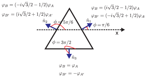
Figure 2: The infinite-mass boundary conditions implemented on the edges of a triangular dot. $\hat{n}_{1},\hat{n}_{2},\hat{n}_{3}$ are the outward unit vectors at each edge of the dot.

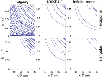
Figure 3: Energy levels of hexagonal (a, c, e) and triangular (b, d, f) graphene quantum dots with zigzag (a, b), armchair (c, d) edges and infinite mass boundary condition (e, f) as function of the square root of the dot area $S$ in the absence of a magnetic field.

III.2 Armchair boundary conditions

The geometry of a hexagonal and triangular graphene quantum dot with armchair edges is illustrated in Figs. 1(a,c). Here, the length of one of the edges of the hexagon dot is $L=(3N_{s}-4)a/2$ and for the triangular dot is $L=3N_{s}a/2$. For an armchair hexagonal graphene dot the total number of C-atoms is $N=[9N_{s}(N_{s}/2-1)+6]$ and for the triangular dot is given by $N=(N_{s}+2)3N_{s}/4$. Note that in the case of armchair boundaries the number of C-atoms in each side is an even number (see Figs. 1(a,c)).

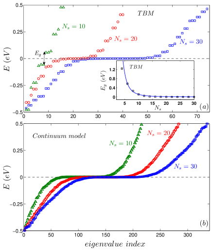
Figure 4: Energy levels of a zigzag hexagonal graphene dot as function of the eigenvalue index obtained by (a) the TBM and (b) the continuum model, for three different sizes of the dot with $N_{s}$ = 10, 20, 30, having respectively surface area $S$ = 14.68, 60.78, 138.32 $nm^{2}$. The inset in panel (a) shows the energy gap $E_{g}$ as function of $N_{s}$ obtained, by the TBM.

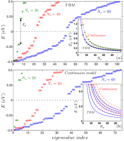
Figure 5: Energy levels of an armchair hexagonal graphene dot as function of the eigenvalue index obtained by (a) the TBM and (b) the continuum model for three different sizes of the dot with $N_{s}$ = 20, 40, 60 having respectively surface area $S$=41.07, 176.23, 405.68 $nm^{2}$. The inset in panel (a) shows the energy gap obtained from both TBM (black squares) and continuum model (green circles). The inset in panel (b) shows the lowest electron energy levels as function of $N_{s}$ for both TBM (blue solid curves) and continuum model (red dashed curves).

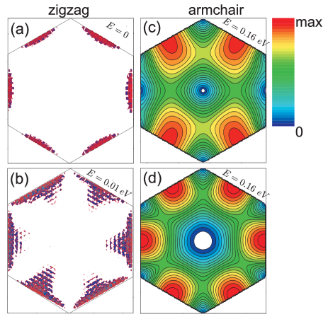
Figure 6: Electron probability densities corresponding to the two lowest energy levels of hexagonal graphene flakes, obtained by the continuum model, for (a,b) zigzag ($N_{s}=20$) and (c,d) armchair ($N_{s}=40$) edges.

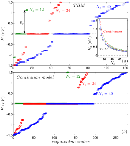
Figure 7: Energy levels of a zigzag triangular graphene dot as function of the eigenvalue index obtained by (a) the TBM and (b) the continuum model for three different sizes of the dot with $N_{s}$ = 12, 24, 40 having respectively surface area $S$=4.42, 16.37, 44.03 $nm^{2}$. The inset in panel (a) shows the energy gap obtained from both TBM (black squares) and continuum model (green circles).

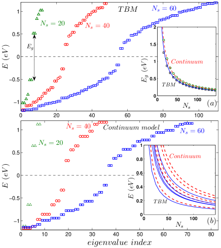
Figure 8: Energy levels of an armchair triangular graphene dot as function of the eigenvalue index obtained by (a) the TBM and (b) the continuum model for three different sizes of the dot with $N_{s}$ = 20, 40, 60 having respectively surface area $S$=7.85, 31.43, 70.72 $nm^{2}$. The inset in panel (a) shows the energy gap obtained from both TBM (black squares) and continuum model (green circles). The inset in panel (b) shows the lowest electron energy levels as function of $N_{s}$ for both TBM (blue solid curves) and continuum model (red dashed curves).

From Figs. 1(a,c), we notice that the edge atoms consist of a line of A-B dimers, where the wave function should be zero. From Eqs. (8a) and (8b), these boundary conditions becomeBrey

$$\varphi_{A}(\boldsymbol{r})=-e^{i(\boldsymbol{K^{\prime}}-\boldsymbol{K})\cdot\boldsymbol{r}}\varphi_{A^{\prime}}(\boldsymbol{r}),$$ (10b)

$$\varphi_{B}(\boldsymbol{r})=-e^{i(\boldsymbol{K^{\prime}}-\boldsymbol{K})\cdot\boldsymbol{r}}\varphi_{B^{\prime}}(\boldsymbol{r}),$$

where $\boldsymbol{r}$ is taken at the position of the edge. Notice that these armchair boundary conditions mix the wave functions of the $K$ and $K^{\prime}$ points.

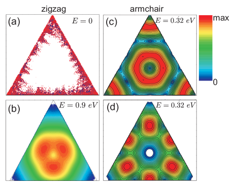
Figure 9: Electron probability densities corresponding to the lowest energy levels of the triangular graphene flakes, obtained by the continuum model, for (a,b) zigzag ($N_{s}=20$) and (c,d) armchair ($N_{s}=40$) edges.

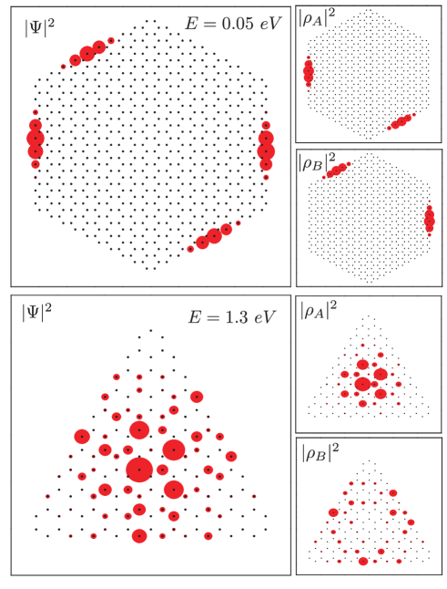
Figure 10: Electron densities for the first energy level of the triangular and hexagonal graphene flakes (using TBM) with $N_{s}=10$ and zigzag edges. Left panels show the total electron density $|\Psi|^{2}$ and the right panels present the electron densities associated with $A$ and $B$ sublattices. The gray dots are the positions of C-atoms.

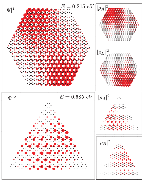
Figure 11: The same as Fig. 10 but for the dots with armchair boundaries and $N_{s}=20$.

III.3 Infinite-mass boundary condition

A mass-related potential energy $V(x,y)$ can be coupled to the Hamiltonian via the $\sigma_{z}$ Pauli matrix,

$$H=v_{F}~{}\boldsymbol{\sigma}.~{}\mathbf{p}+\tau\sigma_{z}V(x,y),$$ (11)

where the parameter $\tau=\pm 1$ distinguishes the two $K$ and $K^{\prime}$ valleys. It is straightforwardly verified that the presence of a mass term in the Hamiltonian of Eq. (11) induces a gap in the energy spectrum of graphene. However, if the mass-related potential $V(x,y)$ is defined as zero inside the dot and infinity at its edge, the Klein tunneling effect at the interface between the internal and external regions of the dot can be avoided and, consequently, the charge carriers will be confined. This infinite-mass boundary condition can be introduced in the Dirac equation by defining $\varphi_{B}(x,y)/\varphi_{A}(x,y)=ie^{i\phi}$ and $\varphi_{B^{\prime}}(x,y)/\varphi_{A^{\prime}}(x,y)=-ie^{i\phi}$ (which, respectively, correspond to the $K$-point and the $K^{\prime}$-point wavespinors) at the boundary, where $\phi$ is the angle between the outward unit vector at the edges and the x-axis. Berry Due to its simplicity, this type of boundary condition has been used in the study of circular graphene dots Schnez and rings Abergel ; Recher2 in the presence of a perpendicularly magnetic field, where analytical solutions can be found. For the hexagonal and triangular geometries the angle $\phi$ has a fixed value at each side of the dot that simplifies the boundary conditions to $\varphi_{B}=\alpha\varphi_{A}$ (for the $K$ valley) and $\varphi_{B^{\prime}}=-\alpha\varphi_{A^{\prime}}$ (for the $K^{\prime}$ valley) where $\alpha=ie^{i\phi}$ is a complex number. The infinite-mass boundary conditions are shown explicitly in Fig. 2 for a triangular dot.

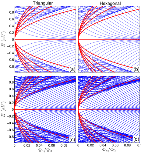
Figure 12: Energy levels of (a,c) triangular and (b,d) hexagonal graphene dots with armchair boundary as function of the magnetic flux threading one carbon hexagon $\Phi_{c}$. The results in panels (a,b) are obtained using the continuum model while panels (c,d) display the TBM results. The quantum dots have an area $S$ such that $\sqrt{S}=10$ nm.

IV Numerical results

IV.1 Zero magnetic field

The energy levels of hexagonal (upper panels) and triangular (lower panels) graphene flakes, as calculated within the continuum model, are shown in Fig. 3 as function of the square root of the dot area. The results are shown for zigzag (a,b), armchair (c,d) and infinite-mass (e,f) boundary conditions and are qualitatively and quantitatively very different. As the dot area increases, the energy levels tend to a gapless spectrum, which is expected, since the energy spectrum of an infinite graphene sheet does not exhibit a gap. A peculiar spectrum is observed for zigzag triangular dots (Fig. 3(b)): zero energy states are found for all sizes of such a dot. These zero energy states are separated from the remaining positive and negative energy states by an energy gap which decreases as the dot becomes larger. The presence of such zero energy states in triangular and trapezoidal graphene flakes have been previously reported in the literature Guclu ; Heiskanen ; Akola , where the TBM was applied. In the case of zigzag triangular dots, it has been shown analyticallyGuclu that the equation $H\Psi=0$ for the TBM Hamiltonian in Eq. (2) leads to $N_{s}-1$ linearly independent states, namely, $N_{s}-1$ degenerate states with $E=0$, for any number $N_{s}$ of C-atoms in one of the edges of the flake. Thus, Fig. 3(b) demonstrates that the existence of zero energy states, which is observed in the TBM, is qualitatively captured by the approximations of the continuum model as well. The results in Fig. 3 also show that the energy levels for a dot with armchair and infinite-mass boundary conditions are qualitative more similar to each other than the spectra for zigzag edges, where carriers are predominantly confined at the edge of the dot. In fact, for the triangular geometry, the infinite mass boundary condition describes very well the armchair states, specially for lower energy states. However, for the hexagonal geometry, the results for armchair and infinite mass boundary conditions are only qualitatively similar where, the hexagonal dots with infinite mass boundary condition exhibit more energy states in comparison with the armchair case.

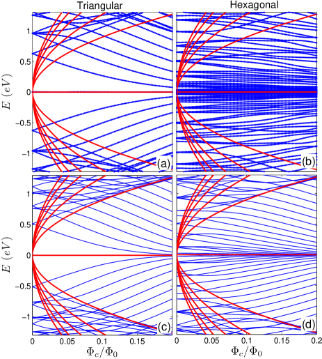
Figure 13: The same as Fig. 12 but for dots with zigzag boundaries and the dots have an area $S$ such that $\sqrt{S}=5$ nm.

Notice that the energy spectra shown in Fig. 3 exhibits degenerate states. These degeneracies, which will be evidenced in the following figures, where we plot the energy spectra as a function of the eigenvalue index, are related to the symmetries of the triangular and hexagonal dots, as we will explain in further detail later on, when we discuss about the electron probability densities.

A comparison between the energy spectra obtained by means of the TBM (a) and the Dirac equation (b) for zigzag hexagonal dots is shown in Fig. 4, for three sizes of the dot, defined by the number of C-atoms in each side of the hexagon $N_{s}$. The energies $E_{i}$ are plotted as a function of the eigenvalue index $i$. Although the results are quantitatively different, they are qualitatively similar, e.g. as the size of the dot increases, they start to exhibit an almost flat energy spectrum as a function of the eigenvalue index around the Dirac point. Such a flat spectrum leads to a peak in the DOS close to the Dirac point, which was recently reported in the literature Zhang for graphene dots with zigzag edges within the TBM. The curves for $N_{s}=30$ obtained by the TBM and continuum models are very similar, except for the fact that many more states are found in the latter, whereas the discrete character of the spectrum in the former is much more clear. For smaller dots, the agreement between these two models becomes clearly worse. For instance, an energy gap $E_{g}$ is found for very small hexagons (i.e. $N_{s}\leq 10$) within TBM, whereas in the case of the continuum model such a gap is extremely small. As a consequence, the continuum model overestimates the DOS at $E=0$ as the dot size decreases, since it exhibits a plateau in the energy as a function of the eigenstate index in the vicinity of $E=0$ even for smaller $N_{s}$, where TBM results show a gap in the energy spectrum. Notice that the $E=0$ states in zigzag dots are edge states, so that the number of zero-energy states depends on the number of edge atoms in the TBM and, similarly, to the number of mesh elements at the edge in the continuum model. Therefore, in the continuum model for $E=0$, the finite elements problem is ill-defined, where the constructed matrix of the finite mesh elements in this case is singular (zero inverse), leading to spurious solutions around $E=0$. As the size of the dot increases, the gap in the TBM results quickly reduces to zero and a zero energy level for the hexagonal flakes with zigzag edges appears.Peres In the inset of Fig. 4(a), the energy gap values obtained by TBM are shown as function of $N_{s}$. These results can be fitted to $E_{g}=\alpha(1/N_{s})^{\gamma}$ (blue solid curve in the inset of Fig. 4(a)), where $\alpha=94.6$ eV and $\gamma=3.23$ are fitting parameters.

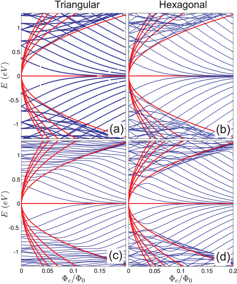
Figure 14: The same as Fig. 12, but for dots with infinite-mass boundary conditions. The dots have an area $S$ such that $\sqrt{S}=5$ nm. In panels (c,d), the infinite-mass boundary condition is applied within the TBM model, where we imposed a +10(-10) eV on-site potential for sublattice A(B) around the dot geometry.

The energy states of armchair hexagonal dots are shown as a function of the eigenvalue index in Fig. 5 within the TBM approach (Fig. 5(a)) and the Dirac-Weyl equations (Fig. 5(b)), for three different sizes of the dot. The energy spectrum in both cases approach the prolonged S-shape curve predicted by EzawaEzawa as the size of the dot increases and the spectrum exhibits an energy gap $E_{g}$ at the Dirac point. The energy gap as function of $N_{s}$ is shown in the inset of Fig. 5(a) which decreases rapidly as the size of the dot increases. Our numerical results can be fitted to $E_{g}=\alpha/N_{s}$ with $\alpha=8.5$ eV for the TBM (blue solid curve) and $\alpha=13$ eV for the continuum model (red dashed curve) results. Notice that $E_{g}$ obtained from the continuum model is larger than the one from the TBM results in particular for small $N_{s}$ and both curves can not be made to coincide by a simple shift in $N_{s}$. This is clearly a consequence of the increased importance of corrections to the linear spectrum used in the continuum model for small sizes of the system. The inset of Fig. 5(b) shows the five lowest electron states for both TBM (blue solid curves) and the continuum model (dashed red curves). Our results show that the continuum model overestimates the energy values also for the upper energy levels in comparison with the TBM energy levels. In fact, the energy dispersion in the continuum model is given by a linear curve, which coincides with the TBM energy spectrum for low energies, but as the energy goes further away from $E=0$, this linear dispersion overestimates the energy as compared to the real band structure of graphene, which starts to bend down from the linear spectrum as the energy increases. This emphasizes once again the importance of the higher order corrections to the linear dispersion, especially for high energy states and smaller dot sizes.

Figure 6 shows the probability density (using the continuum model) corresponding to the first two energy levels of hexagonal flakes. The probability density for the zigzag case with $N_{s}=20$ is presented in panels (a) and (b), respectively, for $E=0$ and $E=0.01$ eV. The results clearly demonstrate that the zero energy states in the zigzag case are due to edge effects and, accordingly, are confined at the edges while the carriers confine towards the center of the flake with increasing energy (see Fig. 6(b)). The probability densities of the armchair edged graphene flake with $N_{s}=40$ are very different as seen in Figs. 6(c,d) for the lowest degenerate states with $E=0.16$ eV. The electron wavefunction is spread out over the whole sample, but different from the usual quantum dots with parabolic energy-momentum spectrum, it has a local minimum in the center of the dot. Note that Fig. 6(c) has only two-fold symmetry while Fig. 6(d) is six-fold symmetric. Both densities are zero in the center, while Fig. 6(c) has two extra zeros at the sides along $y=0$. These results are comparable to the TBM results obtained in Ref.Zhang, .

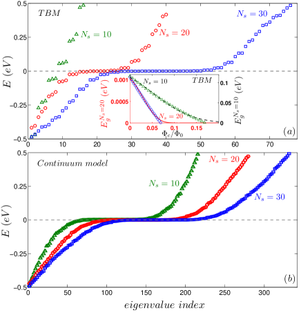
Figure 15: The same as Fig. 3 but in the presence of an external magnetic field of $B=50$ T. The inset shows the energy gap as function of the magnetic flux obtained by the TBM for two values of $N_{s}$. The triangle and circle symbols display Eq. (13) which is fitted to the numerical results.

The energy spectrum for triangular dots with zigzag edges, obtained by the TBM and the Dirac-Weyl equation are shown as a function of the eigenvalue index in Figs. 7(a) and 7(b), respectively. Notice that both energy spectra exhibit zero energy states. As we mentioned before, the number of degenerate states with zero energy is a well defined quantity in the tight-binding approach, namely, $N_{s}-1$, where $N_{s}$ is the number of C-atoms in one side of the triangle Guclu . On the other hand, the result in Fig. 7(b) for the continuum model exhibits many more zero energy states. Therefore, while the continuum model captures qualitatively the existence of zero energy states, it does not provide the appropriate number of degenerate states as calculated by the TBM. These zero energy levels are related to the edge states of zigzag graphene flakes Zhang ; Guclu . The energy gap (between the zero energy level and the first non-zero eigenvalue) is shown in the inset of Fig. 7(a) as function of the size of the dot, where $E_{g}$ obtained by both models are comparable and the difference between the TBM (red dashed curve) and continuum (blue solid curve) results tends to zero for large graphene flakes. These results can be fitted to $E_{g}=\alpha/N_{s}$ with $\alpha=15.75$ eV for the TBM gap and $\alpha=18.9$ eV for the continuum model.

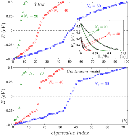
Figure 16: The same as Fig. 4 but in the presence of an external magnetic field of $B=50$ T. The inset shows the energy gap as function of the magnetic flux obtained by the TBM (solid curves) and continuum model (dashed curves) for two values of $N_{s}$. The triangle and circle symbols display Eq. (13) which is fitted to the numerical results.

The energy spectra of triangular dots with armchair edges obtained by the TBM and the continuum model are shown in Fig. 8. No zero energy states are found and the energy gap at the Dirac point for both models is comparable. The gap can be fitted to $E_{g}=\alpha/N_{s}$ ($\alpha=21.9$ eV for TBM and $\alpha=25.9$ eV for the continuum model) as shown respectively by the blue solid and dashed red curves in the inset of Fig. 8(a). The lowest electron energy levels, obtained by the TBM (blue solid curves) and the continuum model (red dashed curves), are shown in the inset of Fig. 8(b) as function of $N_{s}$. The results show a larger difference between the TBM and continuum energy values for the upper energy levels (e.g. $|E^{T}_{1}-E^{C}_{1}|<|E^{T}_{2}-E^{C}_{2}|$).

Notice that the energy gaps found for all the systems that we investigated were fitted to $E_{g}=\alpha/N_{s}$ for different values of $\alpha$, except for the case of zigzag hexagonal dots, where the gap is fitted to $E_{g}=\alpha/N_{s}^{\gamma}$, with $\gamma=3.23$. This is a consequence of the fact that the corners of the zigzag hexagonal dot structure are not terminated by a single atom, as in the case of zigzag triangular dots, but by a pair of C-atoms corresponding to two different sublattices, forming a A-B dimer (see Fig. 1). These A-B dimers are responsible for a vanishing wave function in the corners of the zigzag hexagonal dots, as observed in Fig. 6. As explained in Sec. III A, the zigzag boundary condition for each side of the dot is implemented in the Dirac-Weyl equations by setting to zero the component of the pseudo-spinor corresponding to the sublattice that forms that side. As the sublattice types of adjacent sides of a zigzag hexagonal dot are different, connected by the A-B dimers in the corners, the whole wave function must vanish at these corners, since these points are composed of both A and B sublattices. The vanishing wave function at the corners reduce the effective confinement area and, consequently, increases the energy gap, especially for smaller dots, where the influence of the corners is more significant. As the size of the dot increases, the role of the corners in the energy gap becomes less important and is eventually suppressed by the influence of the zigzag edges, leading to the zero energy states that form the plateau in Fig. 4, explaining the faster decay of the energy gap ($\gamma=3.23$) in zigzag hexagonal dots, as compared to the other cases ($\gamma=1$).

The probability density corresponding to the first two energy levels of triangular graphene flakes, obtained by the continuum model, is shown in Fig. 9. The probability density for the zigzag edged dot with $N_{s}=20$ is presented in panels (a) and (b), respectively, for $E=0$ and for the first non-zero eigenvalue (i.e. $E=0.92$ eV). For the degenerate zero energy states the carriers are confined at the edges of the triangular flake which is typical for zigzag boundaries. States corresponding to large energy values are confined in the center of the triangle (Fig. 9(b)). For armchair triangular flakes, as in the hexagonal case, the electron state is spread out over the whole flake (Figs. 9(c,d) display the different probability densities for $N_{s}=40$ corresponding to the first degenerate eigenvalues with $E=0.32$ eV). Both wavefunctions have three-fold symmetry and the inner part is even six-fold symmetric. Note that the electron density in Fig. 9(d) is zero at the three corners and in the center of the triangle which is different from Fig. 9(c) where zero’s are found at the corners of the inner hexagon and at the center of the sides of this hexagon.

The TBM electron densities of the zigzag graphene dots with $N_{s}=10$ is shown in Fig. 10 for the first energy level of the triangular and hexagonal graphene flake. Left panels present the total electron density $|\Psi^{2}|$ and the electron densities associated with $A$ and $B$ sublattices ($|\rho_{A,B}|^{2}$) are shown in the right panels. We found that the wavefunctions of the two-fold degenerate states are related to each other by a $60^{\circ}$ rotation. The sum of the densities of the degenerate states results in a six-fold (three-fold) symmetric wavefunction for the hexagonal (triangular) flakes. As seen in Fig. 10 the total electron density is related to the densities of $A$ and $B$ sublattices by $|\Psi|^{2}=|\rho_{A}|^{2}+|\rho_{B}|^{2}$. Figure 11 describes the density distributions of the lowest energy levels for armchair graphene flakes. For the armchair hexagonal dots the electron densities corresponding to the $A$ and $B$ sublattices (right panels) can be transformed to each other by a $180^{\circ}$ rotation whereas the density of the triangular wavespinors can not be linked to each other by a rotational transformation.

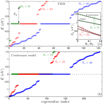
Figure 17: The same as Fig. 5 but in the presence of an external magnetic field of $B=50$ T. The inset shows the energy gap as function of the magnetic flux obtained by the TBM (solid curves) and continuum model (dashed curves) for two values of $N_{s}$. The triangle and circle symbols display Eq. (13) which is fitted to the numerical results.

IV.2 Magnetic field dependence

The dependence of the energy levels of triangular (a) and hexagonal (b) graphene flakes on the magnetic flux through one carbon hexagon $\Phi_{c}=BS_{c}$ is shown in Figs. 12 and 13, respectively for flakes with armchair and zigzag edges. The results in panels (a),(b) are obtained using the continuum model and the results in panels (c),(d) show the TBM energy spectrum. $S_{c}=(3\sqrt{3}/2)a^{2}$ is the area of a carbon hexagon which is indicated by the yellow region in Fig. 1(a). The results are obtained for dots with an area of $S=100$ nm² and $S=25$ nm² respectively for armchair and zigzag edges. The continuum and TBM results are qualitatively similar to each other in the sense that as the magnetic flux increases, the energy levels converge to the Landau levels of a graphene sheet $E_{n}$ (see red solid curves), which are given by

$$E_{n}=sgn(n)\frac{3at}{2l_{B}}\sqrt{2|n|},$$ (12)

where, $l_{B}=\sqrt{\hbar/eB}$ is the magnetic length and $n$ is an integer. The interplay between the quantum dot confinement and the magnetic field confinement is responsible for the appearance of a series of (anti)-crossings in the energy spectrum. As explained earlier, armchair graphene dots do not exhibit zero energy states for $B=0$. However, as the magnetic field increases, some of the excited energy levels approach the zero energy Landau level $n=0$ in both armchair and zigzag graphene flakes, which naturally produces (anti)-crossings between the excited states. Lifting the degeneracy of the energy levels by the magnetic field results in a closing of the energy gap with increasing magnetic field. Notice that the zero energy states of zigzag triangular dots (Fig. 13(a)) are not affected by the magnetic field because they are strongly confined at the edges of the dot. All these features are qualitatively similar to those obtained by the TBM (see the lower panels in Figs. 12,13). In the case of hexagonal zigzag graphene dots (see Fig. 13(b)), the continuum model exhibits a plethora of additional lines as compared to the well known energy spectrum obtained by the TBM (compare Figs. 13(b) and 13(c)).

For the infinite-mass boundary condition, the energy spectrum of triangular (a) and hexagonal (b) dots as a function of the magnetic field is shown in Fig. 14 for the dot with area $S=25$ nm². The energy spectrum in this case differs from both obtained for zigzag and armchair boundary conditions. The spectra exhibit no zero energy state at $B=0$ and show crossings and anti-crossings between the higher energy levels which resemble the TBM results (see Figs. 14(c),(d) respectively for triangular and hexagonal dots). In the TBM model, the infinite-mass boundary conditions can be realized as a graphene dot structure surrounded by an infinite mass media, where we applied a staggered potential (i.e. +10(-10) eV on-site potential for sublattice A(B)) around the dot geometry.

The energy levels obtained by the TBM (a) and the continuum model (b) for hexagonal graphene flakes under a $B=50$ T external magnetic field are shown in Figs. 15 and 16 for zigzag and armchair edges, respectively, as function of the eigenvalue index. The energy spectra of such systems in the absence of magnetic field, which are shown in Figs. 4 and 5, are composed of a series of degenerate states for $|E|>0$. The magnetic field lifts the degeneracy of such states and reduces the gap between the states. The energy gap as function of the magnetic flux through a single carbon hexagon $\Phi_{c}$ is shown in the insets of Fig. 15(a) and Fig. 16(a) respectively for zigzag (with $N_{s}=10,20$) and armchair (with $N_{s}=20,40$) hexagonal dots. These results can be fitted to

$$E_{g}(\Phi_{c}/\Phi_{0})=E_{g}^{0}+E_{g}^{1}(\Phi_{c}/\Phi_{0})+E_{g}^{2}(\Phi_{c}/\Phi_{0})^{2}$$ (13)

where $E_{g}^{0,1,2}$ (eV) are the fitting parameters. In the inset of Figs. 15(a) and 16(a), the fitted results are shown by symbols. The fitting parameters for the TBM results of a zigzag hexagonal dot with $N_{s}=10$ (for the range of $0\leq\Phi_{c}/\Phi_{0}\leq 0.17$ ) are $E_{g}^{0,1,2}=(0.12,-0.91,1.36)$ eV (see triangles in the inset of Fig. 15(a)) and $E_{g}^{0,1,2}=(0.86,-26,210)$ eV, $E_{g}^{0,1,2}=(0.88,-12.5,46.5)$ eV are the fitting parameters of an armchair hexagonal dot with $N_{s}=20$ respectively for TBM and continuum results (triangles in the inset of Fig. 16(a)). The fittings are done for the range of $0\leq\Phi_{c}/\Phi_{0}\leq 0.06$ and $0\leq\Phi_{c}/\Phi_{0}\leq 0.13$ respectively for TBM and continuum results.

For the zigzag case and for $N_{s}=20$, the energy gap is already negligible, whereas for $N_{s}=10$, the $E_{g}\approx 0.12$ eV gap at $B=0$ decays as the magnetic flux increases and approach zero in the limit of large magnetic flux (i.e. $\Phi_{c}/\Phi_{0}>0.2$). Due to the lifting of the degeneracies, the energy spectrum of an armchair hexagonal dot exhibits an almost linear behavior around $E=0$ as function of eigenvalue index where, both TBM and continuum models approximately display the same slope for the linear regime.

For triangular graphene flakes under a $B=50$ T (i.e. $\Phi_{c}/\Phi_{0}=0.0063$) magnetic field, the energy spectra obtained by the TBM (a) and the continuum model (b) are shown in Fig. 17, considering zigzag edges, and Fig. 18, considering armchair edges. As mentioned earlier, the presence of a magnetic field does not affect the $E=0$ edge states in the triangular zigzag flakes, but lifts the degeneracy of the $E\neq 0$ states. The energy gap $E_{g}$ around $E=0$ of triangular flakes is shown as function of magnetic flux $\Phi_{c}$ in the insets of Fig. 17(a) and Fig. 18(a) respectively for zigzag (with $N_{s}=12,24$) and armchair (with $N_{s}=20,40$) edges (circle and triangle symbols present the fitted results). $E_{g}^{0,1,2}=(1.12,-1.32,-0.028)$ and $E_{g}^{0,1,2}=(1.5,-1.77,0.4)$ are the fitting parameters of a zigzag triangular dot with $N_{s}=12$ respectively for TBM and continuum results (see inset of Fig. 17(a)). The fitting parameters for an armchair dot with $N_{s}=20$ (see inset of Fig. 18(a)) obtained by TBM and continuum models are respectively $E_{g}^{0,1,2}=(1.02,-3.87,3.83)$ and $E_{g}^{0,1,2}=(1.12,-2.41,1.2)$. In both zigzag (with $N_{s}=12$ and armchair ($N_{s}=20$) triangular dots the fittings are done for the range of $0\leq\Phi_{c}/\Phi_{0}\leq 0.2$). In contrast with hexagonal dots the energy gap of the triangular dots reduces smoothly (i.e. almost linearly) with increasing the magnetic flux. Therefore the energy gap is weakly affected by a low magnetic field in triangular graphene dots. In the inset of Fig. 18(b) the energy gap is shown as function of $N_{s}$. As in the case of zero magnetic field $E_{g}$ can be fitted to $E_{g}=\alpha/N_{s}$ as function of $N_{s}$ (see blue solid and red dashed curves in Fig. 18(b)). The fitting parameter for $B=50~{}T$ are $\alpha\approx 21.87$ eV for TBM and $\alpha\approx 25.9$ eV for the continuum model which is almost the same as for zero magnetic field (see Fig. 8), i.e. because of the linear magnetic field dependence of the energy gap for low magnetic field it does not affect significantly the dependence of the energy gap on the size of the armchair triangular graphene dot.

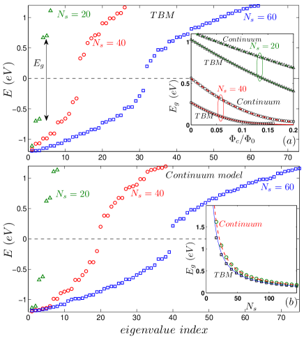
Figure 18: The same as Fig. 6 but in the presence of an external magnetic field $B=50$ T. The inset in panel (a) shows the energy gap $E_{g}$, obtained by the TBM (solid curves) and continuum model (dashed curves), as function of the magnetic flux through one carbon ring $\Phi_{c}$ for $N_{s}=20$ and $N_{s}=40$. The triangle and circle symbols display Eq. (13) which is fitted to the numerical results. In the inset of panel (b) $E_{g}$ is shown as function $N_{s}$ for both TBM (black squares) and continuum models (green circles) in the presence of an external magnetic field $B=50~{}T$.

As a matter of fact, tuning the energy gap by adjusting the external magnetic field is more useful for smaller sizes of the dot, since the energy gap decays to zero as the size of the dot increases. On the other hand, due to the small size of the dots considered in Figs. 15 - 18, we need large magnetic field values (e.g. $B=50$ T) in order to see its effect on the energy spectrum. Nevertheless, as the influence of the magnetic field scales with the magnetic flux through the dot area, similar results will be obtained for lower magnetic fields in case of a larger graphene dot.

V Summary and concluding remarks

We have presented a theoretical study of triangular and hexagonal graphene quantum dots, using the two well known models of graphene: the tight-binding model and the continuum model. For the continuum model, the Dirac-Weyl equations are solved numerically, considering armchair, zigzag and infinite mass boundary conditions. A comparison between the results obtained from the TBM and the Dirac-Weyl equations show the importance of boundary conditions in finite size graphene systems, which affects their energy spectra. The results obtained by the TBM for graphene flakes are only qualitatively similar to the results from the Dirac-Weyl equation for such systems considering zigzag and armchair boundary conditions, which shows that energy values obtained from the continuum model for small graphene dots may not always be quantitatively reliable.

More specifically, for zigzag hexagonal and triangular dots, the DOS at $E=0$ in the absence of a magnetic field is overestimated in the continuum approach. Similarly, the continuum model also overestimates the energy gap around $E=0$ in the armchair case for both geometries. A good agreement between both models is only observed for very large dots, as expected, and such agreement is always better for the triangular case, as compared to the hexagonal case. The energy spectrum obtained using the continuum model with infinite mass boundary condition for hexagonal graphene flakes do not exhibit the same properties as the results obtained with the armchair or zigzag boundaries (in both TBM and continuum models), which shows that this type of boundary condition may not give a good description of finite size hexagonal graphene flakes. On the other hand, for the triangular case, the results from the continuum model with infinite mass boundary conditions describe very well the case of triangular dots with armchair edges.

In the presence of an external magnetic field, the energy levels obtained by the continuum model with zigzag and armchair boundary conditions converge to the Landau levels of graphene as the magnetic field increases, as observed in the TBM. However, many additional artifact states appear in the continuum model, which do not match with any TBM result and do not approach any Landau level. Besides, the influence of an external magnetic field on the gap in the energy spectra of graphene flakes is particulary different for triangular and hexagonal dots. The energy gap of the hexagonal flakes (with $N_{s}\leq 10$) reduces quickly with increasing the magnetic flux, whereas the gap of the triangular flakes decreases smoothly as the magnetic flux increases. This feature is observed in both TBM and continuum model, and suggests that the energy gaps of hexagonal flakes are more easily controllable by an applied external field, as compared to the triangular graphene dots.

- (1) K. S. Novoselov, A. K. Geim, S. V. Morozov, D. Jiang, Y. Zhang, S. V. Dubonos, I. V. Grigorieva, and A. A. Firsov, Science, 306, 666 (2004).
- (2) A. H. Castro Neto, F. Guinea, N. M. R. Peres, K. S. Novoselov, and A. K. Geim, Rev. Mod. Phys. 81, 109 (2009).
- (3) M. I. Katsnelson, K. S. Novoselov, and A. K. Geim, Nat. Phys. 2, 620 (2006).
- (4) J. Milton Pereira, Jr., V. Mlinar, F. M. Peeters, and P. Vasilopoulos, Phys. Rev. B 74, 045424 (2006).
- (5) A. Matulis and F. M. Peeters, Phys. Rev. B 77, 115423 (2008).
- (6) G. Giavaras and F. Nori, App. Phys. Lett. 97, 243106 (2010).
- (7) G. Giavaras and F. Nori, Phys. Rev. B 83, 165427 (2011).
- (8) G. Giavaras, P. A. Maksym and M. Roy, J. Phys.: Condens. Matter 21, 102201 (2009).
- (9) P. Recher, J. Nilsson, G. Burkard, and B. Trauzettel, Phys. Rev. B 79, 085407 (2009).
- (10) K. S. Novoselov, A. K. Geim, S. V. Morozov, D. Jiang, M. I. Katsnelson, I. V. Grigorieva, S. V. Dubonos, and A. A. Firsov, Nature (London) 438, 197 (2005).
- (11) H. Hiura, Appl. Surf. Sci. 222, 374 (2004).
- (12) D. Subramaniam, F. Libisch, C. Pauly, V. Geringer, R. Reiter, T. Mashoff, M. Liebmann, J. Burgdoerfer, C. Busse, T. Michely, M. Pratzer, and M. Morgenstern, arXiv:1104.3875v2 (2011).
- (13) M. Ezawa, Phys. Rev. B 76, 245415 (2007).
- (14) P. Potasz, A. D. Güçlü, and P. Hawrylak, Phys. Rev. B 81, 033403 (2010).
- (15) H. P. Heiskanen, M. Manninen, and J. Akola, New J. Phys. 10, 103015 (2008).
- (16) J. Akola, H. P. Heiskanen, and M. Manninen, Phys. Rev. B 77, 193410 (2008).
- (17) Z. Z. Zhang, K. Chang, and F. M. Peeters, Phys. Rev. B 77, 235411 (2008).
- (18) D. P. Kosimov, A. A. Dzhurakhalov, and F. M. Peeters, Phys. Rev. B 81, 195414 (2010).
- (19) D. A. Bahamon, A. L. C. Pereira, and P. A. Schulz, Phys. Rev. B 79, 125414 (2009).
- (20) K. A. Ritter and Joseph W. Lyding, Nature Materials 8, 235 (2009).
- (21) S. Schnez, K. Ensslin, M. Sigrist, and T. Ihn, Phys. Rev B 78, 195427 (2008); M. Grujic, M. Zarenia, A. Chaves, M. Tadic, G. A. Farias, and F. M. Peeters, Phys. Rev. B 84, 205441 (2011).
- (22) A. V. Rozhkov and F. Nori, Phys. Rev. B 81, 155401 (2010); A. V. Rozhkov, G. Giavaras, Yury P. Bliokh, Valentin Freilikher, and Franco Nori, Physics Reports 503, 77 (2011).
- (23) C. Tang, W. Yan, Y. Zheng, G. Li, and L. Li, Nanotechnology 19, 435401 (2008).
- (24) A. L. Pereira and P. A. Schulz, Phys. Rev. B 78, 125402 (2008).
- (25) For more details see the COMSOL Multiphysics website: www.comsol.com
- (26) A. R. Akhmerov and C. W. J. Beenakker, Phys. Rev. B 77, 085423 (2008).
- (27) L. Brey and H. A. Fertig, Phys. Rev. B 73, 235411 (2006).
- (28) M. V. Berry and R. J. Mondragon, Proc. R. Soc. London, Ser. A 412, 53 (1987).
- (29) D. S. L. Abergel, V. M. Apalkov, and T. Chakraborty, Phys. Rev. B 78, 193405 (2008).
- (30) P. Recher, B. Trauzettel, A. Rycerz, Ya. M. Blanter, C. W. J. Beenakker, and A. F. Morpurgo, Phys. Rev. B 76, 235404 (2007).
- (31) N. M. R. Peres, J. N. B. Rodrigues, T. Stauber, and J. M. B. Lopes dos Santos, J. Phys.: Condens. Matter 21, 344202 (2009).