Lovelock Thin-Shell Wormholes

Abstract

We construct the asymptotically flat charged thin-shell wormholes of Lovelock gravity in seven dimensions by cut-and-paste technique, and apply the generalized junction conditions in order to calculate the energy-momentum tensor of these wormholes on the shell. We find that for negative second order and positive third order Lovelock coefficients, there are thin-shell wormholes that respect the weak energy condition. In this case, the amount of normal matter decreases as the third order Lovelock coefficient increases. For positive second and third order Lovelock coefficients, the weak energy condition is violated and the amount of exotic matter decreases as the charge increases. Finally, we perform a linear stability analysis against a symmetry preserving perturbation, and find that the wormholes are stable provided the derivative of surface pressure density with respect to surface energy density is negative and the throat radius is chosen suitable.

I Introduction

Traversable wormholes are throat like geometrical structures which connect two separate and distinct regions of spacetimes and have no horizon or singularity MT . It is known that the traversable wormholes in Einstein gravity possess a stress-energy tensor that violates the standard energy conditions and therefore they are supported by exotic matter (see, e.g., MTY ). There are two main areas in wormhole research which attracted many authors.

The first one is to try avoiding, as much as possible, the violation of the standard energy conditions. The existence of traversable wormholes that are supported by arbitrarily small quantities of exotic matter viskardad or supported by matter not violating the energy conditions Mart Rich ; Deh1 have been investigated. One of the most interesting kinds of traversable wormholes is the thin-shell wormholes which are constructed by the cut-and-paste technique used for the first time in relation to wormholes in Refs. Vis ; VisP . This is due to the fact that energy is concentrated on the throat of thin-shell wormholes, and therefore the construction of these wormholes needs less exotic matter. Thin-shell wormholes have been investigated by many authors Thin .

The second main research area is the stability analysis of thin-shell wormholes against a symmetry preserving perturbation. This can be done by considering a linearized stability analysis around the static wormhole solutions. The stability analysis will tell whether a static wormhole solution holds under small perturbations or not. The stability analysis of four-dimensional thin-shell wormholes of Einstein gravity with spherical symmetry in vacuum has been done in VisP and in the presence of cosmological constant in Lobo . The generalization of these stability analysis to the case of higher-dimensional wormholes can be found in Lem . Also for stability analysis with dilaton, axion, phantom and other types of matter, and in cylindrical symmetry see Axion .

For thin-shell wormholes of Einstein gravity, the weak energy condition (WEC) is violated. Several attempts have been made to somehow overcome this problem. Some authors resort to the alternative theories of gravity. In this context, the thin-shell wormholes of dilaton gravity supported by Chaplygin gas have been investigated in Dil , of Brans-Dicke theory in Brans and of Gauss-Bonnet gravity in Gauss .

Recently, the third order Lovelock gravity have attracted more attention Deh2 . This is due to the fact that it contains more free parameters, and therefore third order Lovelock gravity may be dual to a more extended class of field theories which one can study with holography Lg3 . Here, we like to add the third order term of Lovelock theory Lov to the gravitational field equations, and investigate the effects of it on the energy conditions and stability of a thin-shell wormhole solution.

In order to do these, one needs the generalized junction conditions in Lovelock gravity. The junction conditions in Einstein gravity is known as Darmois-Israel junction conditions Isr . Also the generalized junction conditions in Gauss-Bonnet gravity Dav and Lovelock gravity Grav have been introduced. In this paper, we use the generalized junction conditions in order to investigate the exoticity of matter on the throat and to perform a linear stability analysis of the thin-shell wormholes of Lovelock gravity.

The paper is organized as follows. In Sec. II, we review the asymptotically flat static charged solutions of third order Lovelock gravity in seven dimensions. Section III is devoted to the generalized junction conditions in Lovelock gravity. We construct the thin-shell wormholes in Sec. IV. In Sec. V, we investigate the energy conditions on shell for these wormhole solutions and we consider the exoticity of matter for different values of the parameters of Lovelock gravity. Finally, we perform the stability analysis of the wormhole solutions in Sec. VI . We finish our paper with some concluding remarks.

II Spherically symmetric geometry

Here, we review the asymptotically flat charged static solutions of third order Lovelock gravity. The action of third order Lovelock gravity in the presence of electromagnetic field may be written as

$$I=\int d^{n+1}x\sqrt{-g}\left(\mathcal{L}_{1}+\alpha_{2}\mathcal{L}_{2}+\alpha_{3}\mathcal{L}_{3}-F_{\mu\nu}F^{\mu\nu}\right)$$ (1)

where $\alpha_{2}$ and $\alpha_{3}$ are second (Gauss-Bonnet) and third order Lovelock coefficients, $\mathcal{L}_{1}=R$ is just the Einstein-Hilbert Lagrangian, $\mathcal{L}_{2}=R_{\mu\nu\gamma\delta}R^{\mu\nu\gamma\delta}-4R_{\mu\nu}R^{\mu\nu}+R^{2}$ is the Gauss-Bonnet Lagrangian, and

$$\mathcal{L}_{3} = 2R^{\mu\nu\sigma\kappa}R_{\sigma\kappa\rho\tau}R_{\phantom{\rho\tau}{\mu\nu}}^{\rho\tau}+8R_{\phantom{\mu\nu}{\sigma\rho}}^{\mu\nu}R_{\phantom{\sigma\kappa}{\nu\tau}}^{\sigma\kappa}R_{\phantom{\rho\tau}{\mu\kappa}}^{\rho\tau}+24R^{\mu\nu\sigma\kappa}R_{\sigma\kappa\nu\rho}R_{\phantom{\rho}{\mu}}^{\rho}$$ (2)

$$+3RR^{\mu\nu\sigma\kappa}R_{\sigma\kappa\mu\nu}+24R^{\mu\nu\sigma\kappa}R_{\sigma\mu}R_{\kappa\nu}+16R^{\mu\nu}R_{\nu\sigma}R_{\phantom{\sigma}{\mu}}^{\sigma}-12RR^{\mu\nu}R_{\mu\nu}+R^{3}$$

is the third order Lovelock Lagrangian. In Eq. (1) $F_{\mu\nu}=\partial_{\mu}A_{\nu}-\partial_{\nu}A_{\mu}$ is electromagnetic tensor field and $A_{\mu}$ is the vector potential.

The seven-dimensional static solution of action (1) may be written as

$$ds^{2}=-f(r)dt^{2}+\frac{dr^{2}}{f(r)}+r^{2}d\Omega_{5}^{2},$$ (3)

where $d\Omega_{5}^{2}$ is the metric of a $5$-sphere, the gauge field is

$$A=\sqrt{\frac{5}{8}}\frac{q}{r^{4}}dt,$$

and the metric function satisfies the following equation

$$24\alpha_{3}(1-f)^{3}+12\alpha_{2}(1-f)^{2}r^{2}+(1-f)r^{4}-m+\frac{q^{2}}{r^{4}}=0.$$ (4)

The solution of Eq. (4) is Deh2005

$$f(r)=1+\frac{\alpha_{2}}{6\alpha_{3}}r^{2}+\frac{1}{12\alpha_{3}}\left(\zeta^{1/3}-\frac{2(\alpha_{3}-2\alpha_{2}^{2})r^{4}}{\zeta^{1/3}}\right),$$ (5)

where $\zeta$ and $\xi$ are

$$\zeta = \xi+\sqrt{\xi^{2}+8(\alpha_{3}-2\alpha_{2}^{2})^{3}r^{12}},$$

$$\xi = 2\alpha_{2}(4\alpha_{2}^{2}-3\alpha_{3})r^{6}-36\alpha_{3}^{2}(m-q^{2}r^{-4}).$$

The above metric presents an asymptotically flat black hole with two horizons provided $q<$ $q_{ext}$, an extreme black hole with one horizon if $q=$ $q_{ext}$ and a naked singularity otherwise, where $q_{ext}$ is

$$q_{ext} = \left\{\frac{2187}{2}\alpha_{2}^{4}-(3\alpha_{3}-\frac{m}{8})(\eta^{2}+243\alpha_{2}^{2})-\frac{3}{2}\alpha_{2}\eta^{3}\right\}^{1/2},$$

$$\eta = \left(2m+81\alpha_{2}^{2}-48\alpha_{3}\right)^{1/2}.$$ (6)

The metric function for the special case $\alpha_{3}=2{\alpha_{2}}^{2}=\alpha^{2}/72$ reduces to

$$f(r)=1+{\frac{{r}^{2}}{\alpha}}\left\{1-\left({1+\frac{3\alpha m}{r^{6}}-\frac{3\alpha{q}^{2}}{r^{10}}}\right)^{1/3}\right\}.$$ (7)

In studying wormholes, the matter is outside the horizon $r>r_{h}$, where $r_{h}$ is the largest real root of $f(r)=0$.

III Junction Conditions in Lovelock Gravity

The action of Lovelock gravity with well-defined variational principle in $n+1$ dimension may be written as DBS

$$I_{G} = \kappa\int d^{n+1}x\sqrt{-g}\sum_{p=0}^{[n/2]}\alpha_{p}\mathcal{L}_{p}$$ (8)

$$-2\kappa\int_{\Sigma}d^{n}x\sqrt{-\gamma}\sum_{p=0}^{[n/2]}\sum_{s=0}^{p-1}\frac{(-1)^{p-s}p\alpha_{p}}{2^{s}(2p-2s-1)}\mathcal{H}^{(p)}$$

where $[z]$ denotes the integer part of $z$, $\alpha_{p}$ is Lovelock coefficient, $\mathcal{L}_{p}$ is the Euler density of a $2p$-dimensional manifold

$$\mathcal{L}_{p}=\frac{1}{2^{p}}\delta_{\rho_{1}\sigma_{1}\cdots\rho_{p}\sigma_{p}}^{\mu_{1}\nu_{1}\cdots\mu_{p}\nu_{p}}R_{\mu_{1}\nu_{1}}^{\phantom{\mu_{1}\nu_{1}}{\rho_{1}\sigma_{1}}}\cdots R_{\mu_{p}\nu_{p}}^{\phantom{\mu_{k}\nu_{k}}{\rho_{p}\sigma_{p}}},$$ (9)

and

$$\mathcal{H}^{(p)}=\delta_{\,[b_{1}\ldots b_{2p-1}]}^{[a_{1}\ldots a_{2p-1}]}R_{\phantom{b_{1}b_{1}}{a_{1}a_{2}}}^{b_{1}b_{2}}\cdots R_{\phantom{b_{2s}}{a_{2s-1}a_{2s}}}^{b_{2s-1}b_{2s}}\Theta_{a1}^{b1}\cdots\Theta_{a_{2p-1}}^{b_{2p-1}}$$ (10)

In the above equations $\delta_{\rho_{1}\sigma_{1}\cdots\rho_{p}\sigma p}^{\mu_{1}\nu_{1}\cdots\mu p\nu_{p}}$ is the generalized totally antisymmetric Kronicker delta and $\gamma_{ab}$ and $\Theta_{ab}$ are the induced metric and extrinsic curvature of the timelike hypersurface $\Sigma$.

Varying the action (8) with respect to the induced metric $\gamma_{ab}$ gives DBS ; Grav

$$\mathcal{T}_{b}^{a}=-2\kappa\sum_{p=0}^{n}\sum_{s=0}^{p-1}\frac{4^{p-s}p!\alpha_{p}}{2^{p+1}s!(2p-2s-1)!!}\mathcal{H}_{\phantom{i}b}^{(p,s)a}$$ (11)

where $\mathcal{H}_{\phantom{i}b}^{(p,s)a}$ is

$$\mathcal{H}_{\phantom{i}b}^{(p,s)a}=\delta_{\,[b_{1}\ldots b_{2p-1}b]}^{[a_{1}\ldots a_{2p-1}a]}R_{\phantom{b_{1}b_{2}}{a_{1}a_{2}}}^{b_{1}b_{2}}\cdots R_{\phantom{b_{2s-1}b_{2s}}{a_{2s-1}a_{2s}}}^{b_{2s-1}b_{2s}}\Theta_{a_{2s+1}}^{b_{2s+1}}\cdots\Theta_{a_{2p-1}}^{b_{2p-1}}.$$ (12)

In Eqs. (10) and (12) $R_{abcd}$ is the boundary components of the Riemann tensor of the Manifold $\mathcal{M}$ which is related to the intrinsic curvature of the hypersurface $\Sigma$, $\hat{R}_{abcd}(\gamma)$, through the Gauss-Codazzi equation as

$$R_{abcd}=\hat{R}_{abcd}(\gamma)+\Theta_{ac}\Theta_{bd}-\Theta_{ad}\Theta_{bc}$$

Now considering the manifold $\mathcal{M}$ as two manifold $\mathcal{M}_{+}$ and $\mathcal{M}_{-}$ separated by hypersurface $\Sigma$, and denoting its two sides by $\Sigma_{\pm}$, then the generalized junction conditions can be written as

$$\mathcal{S}^{ab}=\mathcal{T}_{+}^{ab}-\mathcal{T}_{-}^{ab},$$ (13)

where $\mathcal{T}_{\pm}^{ab}$ is the energy-momentum tensor given in Eq. (12) associated with the two sides of the shell.

IV Thin-shell Wormhole Construction

To construct a thin-shell wormhole in third order Lovelock gravity, we use the well-known cut-and-pase technique. Taking two copies of asymptotically flat solutions of Lovelock gravity given by Eqs. (3) and (5) and removing from each manifold the seven-dimensional region described by

$$\Omega_{\pm}=\left\{r_{\pm}\leq a;\ \ \ a>r_{h}\right\}$$ (14)

we are left with two geodesically incomplete manifolds with the following timelike hypersurface as boundaries

$$\Sigma_{\pm}=\left\{r_{\pm}=a;\ \ \ a>r_{h}\right\}.$$ (15)

Now identifying these two boundaries, $\Sigma_{+}=\Sigma_{-}=\Sigma$, we leave with a geodesically complete manifold containing the two asymptotically flat regions $\Omega_{+}$ and $\Omega_{-}$ which are connected by a wormhole. The throat of the wormhole located at $\Sigma$ with metric

$$ds_{\Sigma}^{2}=-d\tau^{2}+a^{2}(\tau)d\Omega_{5}^{2},$$

where $\tau$ is the proper time along the hypersurface $\Sigma$ and $a(\tau)$ is the radius of the throat. All the matter is concentrated on $\Sigma$.

To analyze such a thin-shell configuration, we need to use the modified junction condition introduced in Sec. III. Denoting the coordinates on $\Sigma$ by $\xi^{a}=(\tau,\theta^{i};$ $i=1...5)$, the extrinsic curvature associated with the two sides of the shell are

$${\mathcal{K}}_{ab}^{\pm}=-n_{\rho}^{\pm}\left(\frac{\partial^{2}X^{\rho}}{\partial\xi^{a}\partial\xi^{b}}+\Gamma_{\mu\nu}^{\rho}\frac{\partial X^{\mu}}{\partial\xi^{a}}\frac{\partial X^{\nu}}{\partial\xi^{b}}\right)_{r=a},$$ (16)

where $n_{\rho}^{\pm}$ are the units normal ($n_{\rho}n^{\rho}=1$) to the surface $\Sigma$ in $\mathcal{M}$:

$$n_{\gamma}^{\pm}=\pm\left|g^{\mu\nu}\frac{\partial\mathcal{G}}{\partial X^{\mu}}\frac{\partial\mathcal{G}}{\partial X^{\nu}}\right|\frac{\partial\mathcal{G}}{\partial X^{\gamma}}$$ (17)

and $\mathcal{G}(r,\tau)$ is the equation of the boundary $\Sigma$:

$$\mathcal{G}(r,\tau)=r-a(\tau)=0.$$ (18)

Using an orthonormal basis $\{e_{\hat{\tau}},e_{\hat{\imath}};$ $i=1...5\}$, the components of extrinsic curvature tensor may be calculated as

$$\mathcal{K}_{~{}\hat{\tau}}^{\hat{\tau}}=\frac{\Gamma}{\Delta},\hskip 28.45274pt\mathcal{K}_{\hat{\jmath}}^{\hat{\imath}}=\frac{\Delta}{a}~{}\delta_{\hat{\jmath}}^{\hat{\imath}},$$ (19)

where

$$\Gamma=\ddot{a}+\frac{f^{\prime}\left(a\right)}{2},\text{ \ \ \ }\Delta=\sqrt{\dot{a}^{2}+f\left(a\right),}$$

and prime and overdot denote the derivative with respect to $a$ and $\tau$, respectively. Equation (19) shows that the form of the stress-energy tensor on the shell is ${S}_{~{}\hat{b}}^{\hat{a}}=~{}\mbox{diag}~{}(-\sigma,p~{}\delta_{\hat{\jmath}}^{\hat{\imath}})$, where $\sigma$ is the surface energy density and $p$ is the transverse pressure.

Now using the junction condition (13), the components of energy momentum tensor on the shell may be written as

$$\sigma = -S_{\hat{\tau}}^{\hat{\tau}}=-\frac{\Delta}{4\pi a}\left\{5+\frac{40\alpha_{2}}{a^{2}}[3(1+\dot{a}^{2})-\Delta^{2}]\ +\frac{24\alpha_{3}}{a^{4}}[15(1+\dot{a}^{2})^{2}-10\Delta^{2}(1+\dot{a}^{2})+3\Delta^{4}]\right\},$$

$$p = S_{\hat{i}}^{\hat{i}}=\frac{1}{8\pi}\Bigg{\{}\frac{2\Gamma}{\Delta}+\frac{8\Delta}{a}+\frac{16\alpha_{2}}{a^{2}}\left[\frac{3\Gamma}{\Delta}\left(1+\dot{a}^{2}-\Delta^{2}\right)+\frac{2\Delta}{a}\left[3\left(1+\dot{a}^{2}\right)-\Delta^{2}\right]+6\ddot{a}\Delta\right]$$ (20)

$$+\frac{48\alpha_{3}}{a^{4}}\left[\frac{3\Gamma}{\Delta}\left(1+\dot{a}^{2}-\Delta^{2}\right)^{2}+4\ddot{a}\Delta\left[3(1+\dot{a}^{2})-\Delta^{2}\right]\right]\Bigg{\}}.$$

One may note that the surface energy density and transverse pressure satisfy the energy conservation equation:

$$\frac{d}{d\tau}\left(\sigma a^{5}\right)+p\frac{d}{d\tau}\left(a^{5}\right)=0.$$ (21)

The first term in Eq. (21) represents the internal energy change of the throat and the second term shows the work done by the throat’s internal forces.

V Exoticity of the Matter on Shell

In this section, we consider the issue of energy condition on the shell for the case of static configurations with $a=a_{0}$ and $\dot{a}=\ddot{a}=0$. In our case the weak energy condition is satisfied provided $\sigma\geq 0$, and $\sigma+p\geq 0$. Using Eqs. (20) one obtains

$$\sigma_{0} = -\frac{1}{8\pi a_{0}\sqrt{f_{0}}}\left\{10f_{0}+\frac{80\alpha_{2}}{a_{0}^{2}}f_{0}(3-f_{0})+\frac{48\alpha_{3}}{a_{0}^{4}}f_{0}(15-10f_{0}+3f_{0}{}^{2})\right\},$$ (22)

$$\sigma_{0}+p_{0} = \frac{1}{8\pi a_{0}\sqrt{f_{0}}}\Bigg{\{}(-2f_{0}+a_{0}f_{0}^{\prime})+\frac{8\alpha_{2}}{a_{0}^{2}}\{3a_{0}f_{0}^{\prime}(1-f_{0})$$ (24)

$$-6f_{0}(3-f_{0})\}+\frac{24\alpha_{3}}{a_{0}^{4}}\{3a_{0}f_{0}^{\prime}(1-2f_{0}+f_{0}^{2})-2f_{0}(15-10f_{0}+3f_{0}{}^{2})\}\Bigg{\}},$$

where $f_{0}=f(a_{0})$ and $f_{0}^{\prime}=f^{\prime}(a_{0})$. In contrast to the case of an Einsteinian thin-shell wormhole for which $\sigma<0$ and therefore the weak energy condition is violated Lem , here we can have thin-shell wormholes with normal matter on shell. In order to investigate the exoticity of the matter, we calculate the amount of matter on shell which is

$$\digamma=\int drd\Omega_{5}[\sigma_{0}\delta(r-a_{0})+p_{r}].$$ (25)

For our case, the shell does not exert radial pressure, $p_{r}=0$, and therefore the amount of matter on shell is

$$\digamma=\pi^{3}a_{0}^{5}\sigma_{0}=\pi^{2}\sqrt{f_{0}}\left\{-\frac{5}{4}a_{0}^{4}+10\alpha_{2}a_{0}^{2}(-3+f_{0})+6\alpha_{3}\left(-15+10f_{0}-3f_{0}^{2}\right)\right\}.$$ (26)

In Einstein gravity, $\alpha_{2}=\alpha_{3}=0$, the matter is exotic both for Reissner-Nordstrom $(Q\neq 0)$ and Schwarzschild $(Q=0)$ thin-shell wormholes as one can see from Eq. (26). In Gauss-Bonnet gravity ($\alpha_{3}=0$) with $\alpha_{2}<0$, one may have thin-shell wormholes supported by normal matter Mazha .

Now, we investigate the condition that thin-shell wormhole may be supported by normal matter in third order Lovelock gravity. For the special case $\alpha_{3}=2{\alpha_{2}}^{2}=\alpha^{2}/72$ , Eq. (26) shows that $\digamma<0$, and therefore the on shell matter is exotic. But, one can choose the parameters of the metric function such that the amount of exotic matter on the throat to be as less as possible. For instance, as one can see in Fig. 1, the amount of exotic matter decreases as $q$ increases.

For the general solutions of third order Lovelock gravity with positive values of $\alpha_{2}$ and $\alpha_{3}$, the matter on the shell is exotic as one can see in Fig. 2. But, for $\alpha_{3}>0$ and $\alpha_{2}<0$, $\digamma$ can be positive and therefore the matter may be normal, as one can see in Fig 3. For this case as Fig 4 shows, there exists a region with $\sigma_{0}\geq 0$ and $\sigma_{0}+p_{0}\geq 0$ and therefore WEC is are satisfied. Since $0<f_{0}<1$, the factor of $\alpha_{3}$ in Eq. (26), $-15+10f_{0}-3f_{0}^{2}$, is negative and therefore the amount of normal matter for negative $\alpha_{2}$ decreases as $\alpha_{3}$ increases. Also, in this case the amount of normal matter decreases as the charge $q$ increases.

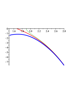
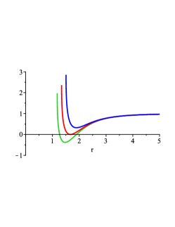
Figure 1: Right: $f(r)$ versus $r$; Left: $\digamma/100$ versus $a_{0}$ for $\alpha=1$, $m=20$, $q>q_{ext}$, $q=q_{ext}$ and $q<q_{ext}$ from up to down, for the right figure and down to up for the left figure, respectively.

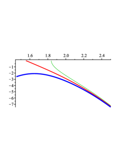
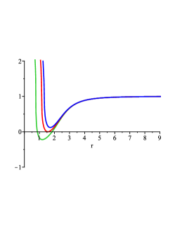
Figure 2: Right: $f(r)$ versus $r$; Left: $\digamma/100$ versus $a_{0}$ for $\alpha_{2}=0.2$, $\alpha_{3}=0.4$, $m=30$, $q>q_{ext}$, $q=q_{ext}$ and $q<q_{ext}$ from up to down, for the right figure and down to up for the left figure, respectively.

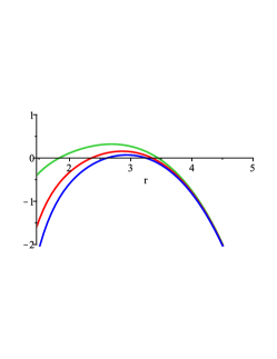
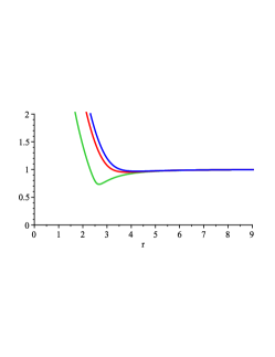
Figure 3: Right: $f(r)$ versus $r$; Left: $\digamma/1000$ versus $a_{0}$ for $\alpha_{2}=-0.8$, $\alpha_{3}=0.5$, $m=20$, $q=57$, 46.5 and 23.72 from up to down, for the right figure and down to up for the left figure, respectively.

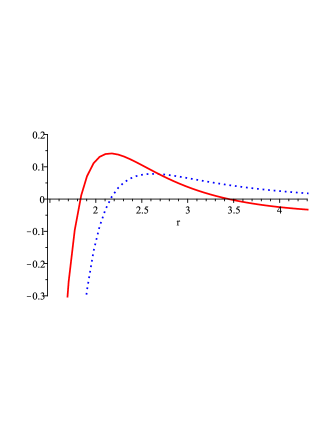
Figure 4: $\sigma_{0}$ (line) and $\sigma_{0}+p_{0}$ (dotted) versus $r$ for $\alpha_{2}=-0.8$, $\alpha_{3}=0.5$, $m=20$ and $q=23.72$.

VI STABILITY ANALYSIS

In this section, we perform a stability analysis under a linear perturbation such that the spherical symmetry of the wormhole configuration is preserved. To analyze the stability, we use a cold equation of state $p=p(\sigma)$ with $\eta=dp/d\sigma$. We consider a small radial perturbation around a static solution with radius $a_{0}$. In this case, one may write $p\simeq p_{0}+\eta_{0}(\sigma-\sigma_{0})$, where $p_{0}$, $\sigma_{0}$ and $\eta_{0}$ are the transverse pressure, surface energy density and $(dp/d\sigma)$ at $a=a_{0}$, respectively. Using this linear equation of state and Eq. (21), one obtains

$$\sigma\left(a\right)=\left(\frac{\sigma_{0+}p_{0}}{1+\eta_{0}}\right)\left(\frac{a_{0}}{a}\right)^{5\left(1+\eta_{0}\right)}+\frac{\eta_{0}\sigma_{0-}p_{0}}{1+\eta_{0}}.$$ (27)

Now Eq. (20), which is the equation of motion for the radius of the throat, can be written as

$$5a^{4}+40\alpha_{2}a^{2}\left[2(1+\dot{a}^{2})+1-{f(a)}\right]+24\alpha_{3}\Big{\{}8(1+\dot{a}^{2})^{2}$$

$$+4[1-f(a)](1+\dot{a}^{2})+3[1-f(a)]^{2}]\Big{\}}=-\frac{4\pi a^{5}\sigma(a)}{\sqrt{\dot{a}^{2}+f(a)}},$$ (28)

where $\sigma(a)$ is given in Eq. (27).

In principle, one may solve Eq. (28) for $\dot{a}^{2}$ and obtain the potential $V(a)$ in the equation $\dot{a}^{2}=-V(a)$. Then, the wormhole with radius $a_{0}$ is linearly stable provided the potential $V(a)$ is negative and minimum at $a=a_{0}$. In third order Lovelock gravity, one encounters with a fifth order algebraic equation for $\dot{a}^{2}$ and therefore one may perform stability analysis numerically. Numerical calculations are shown in Figs. 5 and 6. As these figures show, the wormholes are stable provided the derivative of surface pressure density with respect to surface energy density at the throat, $\eta_{0}$, is negative and the throat radius $a_{0}$ is chosen suitable.

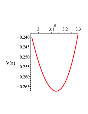
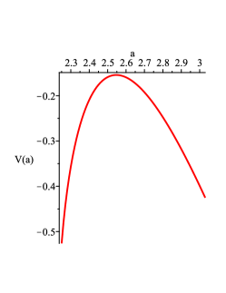
Figure 5: $V(a)$ versus $a$ for $\alpha_{2}=-0.8$, $\alpha_{3}=0.5$, $m=20$, $q=23.72$, and $\eta=1.2$ (right); $\eta=-1.8$ (left).

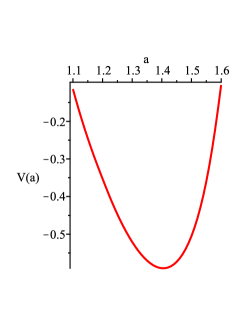
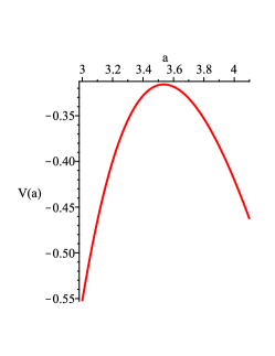
Figure 6: $V(a)$ versus $a$ for $\alpha_{2}=0.2$, $\alpha_{3}=0.4$, $m=30$, $q=7.9$ and $\eta=0.9$ (right); $\eta=-1.8$ (left).

VII CLOSING REMARKS

In this paper, we first use the well-known cut-and-pase technique, and constructed the asymptotically flat thin-shell wormholes of Lovelock gravity in seven dimensions. We calculated the components of energy momentum tensor on shell through the use of the general junction condition. We found that the matter on the throat is exotic if both $\alpha_{2}$ and $\alpha_{3}$ are positive. However, the amount of exotic matter on shell reduces as the charge of the wormhole increases. In the case of negative $\alpha_{2}$ and positive $\alpha_{3}$, one may have a region for the throat radius with $\sigma_{0}\geq 0$ and $\sigma_{0}+p_{0}\geq 0$, and therefore WEC is satisfied. That is, one may have wormholes with normal matter provided $\alpha_{2}<0$ and $\alpha_{3}>0$. In this case, the amount of normal matter decreases as the third order Lovelock parameter increases. Finally, we applied a linear stability analysis against symmetry preserving perturbation and found that the wormholes with suitable throat radius are stable provided $\eta_{0}=(dp/d\sigma)_{a_{0}}<0$.

References

• (1) M. S. Morris and K. S. Thorne, Am. J. Phys. 56, 395 (1986).
• (2) M. S. Morris, K. S. Thorne, and U. Yurtsever, Phys. Rev. Lett. 61, 1446 (1988); M. Visser, Lorentzian Wormholes: From Einstein to Hawking (American Institute of Physics, New York, 1995).
• (3) M. Visser, S. Kar and N. Dadhich, Phys. Rev. Lett. 90, 201102 (2003).
• (4) M. G. Richarte, Phys. Rev. D 82, 044021 (2010).
• (5) M. H. Dehghani and Z. Dayyani, Phys. Rev. D 79, 064010 (2009).
• (6) M. Visser, Phys. Rev. D 39, 3182 (1989); Nucl. Phys. B 328, 203 (1989).
• (7) E. Poisson and M. Visser, Phys. Rev. D 52, 7318 (1995).
• (8) S. W. Kim, Phys. Lett. A 166, 13 (1992); F. S. N. Lobo, Class. Quant. Grav. 21, 4811 (2004); J. P. S. Lemos and F. S. N. Lobo, Phys. Rev. D 69, 104007 (2004); E. F. Eiroa and C. Simeone, ibid. 70, 044008 (2004); E. F. Eiroa and C. Simeone, ibid. 71, 127501 (2005); F. Rahaman, M. Kalam, and S. Chakraborty, Gen. Relativ. Gravit. 38, 1687 (2006); C. Bejarano, E. F. Eiroa, and C. Simeone, Phys. Rev. D 75, 027501 (2007); F. Rahaman, M. Kalam, and S. Chakraborty, Int. J. Mod. Phys. D 16, 1669 (2007); F. Rahaman, M. Kalam, K. A. Rahman, and S. Chakraborty, Gen. Relativ. Gravit. 39, 945 (2007); E. Gravanis and S. Willison, Phys. Rev. D 75, 084025 (2007); M. G. Richarte and C. Simeone, Int. J. Mod. Phys. D 17, 1179 (2008).
• (9) F. S. N. Lobo and P. Crawford, Class. Quant. Grav. 21, 391 (2004).
• (10) F. Rahaman, M. Kalam, and S. Chakraborty, Gen. Relativ. Gravit. 38, 1687 (2006); J. P. S. Lemos and F. S. N. Lobo, Phys. Rev D 78, 044030 (2008); G. A. S. Dias and J. P. S. Lemos, arXiv:1008.3376.
• (11) E. F. Eiroa, Phys. Rev. D 78, 024018 (2008); A. A. Usmani, F. Rahaman, S. Ray, Sk. A. Rakib, and Z. Hasan, Gen. Relativ. Gravit. 42, 2901 (2010); P. K. F. Kuhfittig, Acta Phys. Polonica B,41, 2017 (2010); E. F. Eiroa and C. Simeone, Phys. Rev. D 81, 084022 (2010).
• (12) C. Bejarano and E. F. Eiroa, Phys. Rev. D 84, 064043 (2011).
• (13) X. Yue and S. Gao, Phys. Lett. A 375, 2193 (2011); Francisco S. N. Lobo, Miguel A. Oliveira, Phys. Rev. D 81, 067501 (2010).
• (14) E. Gravanis and S. Willison, Phys. Rev. D 75, 084025 (2007); G. Dotti, J. Oliva, and R. Troncoso, ibid. 76, 064038 (2007); H. Maeda and M. Nozawa, ibid. 78, 024005 (2008); M. Richarte and C. Simeone, ibid. 76, 087502 (2007); Erratum-ibid. D 77, 089903 (2008); M. Thibeault, C. Simeone, and E. F. Eiroa, Gen. Relativ. Gravit. 38, 1593 (2006).
• (15) M. H. Dehghani and R. Pourhasan, Phys. Rev. D 79, 064015 (2009); M.H. Dehghani and R.B. Mann, J. High Energy Phys. 07, 019 (2010); M. H. Dehghani and Sh. Asnafi, Phys. Rev. D 84, 064038 (2011).
• (16) X.H. Ge, S.J. Sin, S.F. Wu and G.H. Yang, Phys. Rev. D 80, 104019 (2009); J. de Boer, M. Kulaxizi and A. Parnachev, J. High Energy Phys. 06, 008 (2010); X.O. Camanho and J. D. Edelstein, [arXiv:0912.1944]; F. W. Shu, Phys. Lett. B 685, 325 (2010).
• (17) D. Lovelock, J. Math. Phys. 12, 498n (1971); D. Lovelock, Aequationes Math. 4, 127 (1970).
• (18) W. Israel, Nuovo Cimento 44B, 1 (1966); N. Sen, Ann. Phys. (Leipzig) 73, 365 (1924); K. Lanczos, ibid. 74, 518 (1924); G. Darmois, Mémorial des Sciences Mathématiques, Fascicule XXV ch. V (Gauthier-Villars, Paris, 1927).
• (19) S. C. Davis, Phys. Rev. D 67, 024030 (2003).
• (20) E. Gravanis and S. Willison, J. Geom. Phys. 57, 1861 (2007); O. Miskovic and R. Olea, J. High Energy Phys. 10, 28 (2007).
• (21) M. H. Dehghani and M. Shamirzaie, Phys. Rev. D 72, 124015 (2005).
• (22) C. Teitelboim and J. Zanelli, Class. and Quant.Grav. 4, L125 (1987); M. H. Dehghani, N. Bostani, A. Sheykhi, Phys. Rev. D 73, 104013 (2006).
• (23) S. Habib Mazharimousavi, M. Halilsoy and Z. Amirabi, Phys. Rev. D 81, 104002 (2010); Class. Quant. Grav. 28, 025004 (2011).