Fast generation of multiparticle entangled state for flux qubits in a circle array of transmission line resonators with tunable coupling

Abstract

We study a one-step approach to the fast generation of Greenberger-Horne-Zeilinger (GHZ) states in a circuit QED system with superconducting flux qubits. The GHZ state can be generated in about $10$ ns, which is much shorter than the coherence time of flux qubits and comparable with the time of single-qubit operation. In our proposal, a time-dependent microwave field is applied to a superconducting transmission line resonator (TLR) and displaces the resonator in a controlled manner, thus inducing indirect qubit-qubit coupling without residual entanglement between the qubits and the resonator. The design of a tunably coupled TLR circle array provides us with the potential for extending this one-step scheme to the case of many qubits coupled via several TLRs.

I Introduction

Entanglement lies at the heart of quantum mechanics and plays a key role in quantum information processing. In quantum error correction, quantum teleportation and quantum cryptography, the generation of high fidelity multi-particle entangled states, such as the Greenberger-Horne-Zeilinger (GHZ) state or two qubit Bell state, is required Nielsen . Therefore, the preparation and verification of the entangled states are of great practical importance in quantum information processing systems.

Superconducting qubits MSS ; you-nature are the most promising candidate for realizing solid-state quantum information processing. Generation of the GHZ state in superconducting quantum circuits is consequently a highly important issue. While 14-particle and 10-particle entanglement have been experimentally demonstrated in trapped-ion systems Monz2011 and photonic systems Gao2010 , respectively, theoretical studies have focused on generating the three-qubit GHZ state in superconducting charge wei2006 , flux kim2008 and phase Galiautdinov2008 qubit circuits with direct qubit-qubit interaction. Experimental demonstrations of entanglement have also been limited to the cases of the two berkley2003 ; izamalkov2004 ; Niskanen2007 ; Plantenberg2007 or three xu2005 ; Neeley2010 ; DiCarlo2010 ; altomare2010 ; Fedorov2011 particles so far. Therefore, how to generate multiqubit GHZ states in superconducting quantum circuits is still an open question.

The circuit QED system Girvin2008 provides a possibly scalable method of realizing quantum information processing with superconducting qubits. In such a system, the quantized microwave field can act as a data bus to transfer information between qubits. The generation of a multiparticle (three or more particles) GHZ state using the system of the circuit QED has been proposed in Refs. Zhu2005, ; Helmer2009, ; Bishop2009, ; Hutchison2009, ; Tsomokos2008, ; Wang2010, . However, the generation of the GHZ state in Refs. Helmer2009, ; Bishop2009, ; Hutchison2009, is based on measurement, and is thus probabilistic. The probability of generation of the GHZ state exponentially decreases with the number of qubits. The proposal in Ref. Wang2010, , which is similar to that for trapped-ion systems Molmer1999 ; Sorensen2000 and atomic systems Solano2003 ; Zheng2003 , comprises deterministic generation of the GHZ state in a system of either flux qubits or charge qubits. However, it is difficult to realize this approach in current experiments due to the existence of a few practical problems, as follows. First, to prepare a high-fidelity GHZ state, the time control of the dc current pulse should be precisely set around $2\pi/\omega_{r}$, where $\omega_{r}$ is the frequency of the fundamental cavity mode and the usual range is from $2\pi\times 1$ GHz to $2\pi\times 10$ GHz. It is a major technical challenge to carry out the proposed experiment with the present time resolution of high-performance commercial arbitrary waveform generator, which is generally about $1$ ns. Furthermore, changes in the half of the flux quantum in an $\alpha$ loop (defined in Sec. II) with a typical area, for example, $10\,\mu m^{2}$ also represent a technical problem, because it is necessary to apply a biased current up to $1\,$mA via on-chip biased line in an ultra-low temperature environment if the mutual inductance between the $\alpha$ loop and the biased line is $\sim 1\,$pH. Second, the preparation time is one or even two orders of magnitude longer than that of the single-qubit operation. Faster preparation requires reduction of the frequency of the fundamental cavity mode. This may lead to more operational errors arising from the thermal excitations in the cavity. Third, the number of superconducting flux qubits that can be placed around current anti-node point of the one-dimensional superconducting transmission line resonator (TLR) is limited, and thus the proposed scalable method for many qubits remains an open question.

To overcome the problems encountered in previous studies (e.g., in Ref. Wang2010, ) and make the proposal experimentally more feasible, we introduce a one-step multi-qubit GHZ state generation method in the system of a circuit QED with flux qubits. The advantages of our proposal are as follows. 1) The classical driving field is directly applied to the TLR, in contrast to the usual case in which the driving field is separately applied to the qubits. Thus, the interactions between the qubits and the classical field are induced by coherently displacing the cavity field. This facilitates experiments not only to obtain homogenous coupling constants, but also to realize synchronization of the driving on different qubits. 2) The generation time can be as short as the single-qubit operation time. 3) Our proposal can be extended a case of many qubits case by using a coupled TLR array as a data bus. We expect that our proposal will work well for more than $20$ qubits from our current experiments with the simplest setup, in which the flux qubits are placed inside two tunably coupled TLRs via a dc-SQUID.

Our paper is organized as follows. In Sec. II, one-step generation of the GHZ state in flux qubits coupled to a TLR system is presented using both analytical and numerical analysis. In Sec. III, one-step generation of the GHZ state in flux qubits coupled to two or more TLRs with tunable coupling is discussed. Finally, discussion and conclusion are presented in Sec. IV.

II A GHZ state generation for flux Qubits inside a cavity

II.1 Theoretical Model

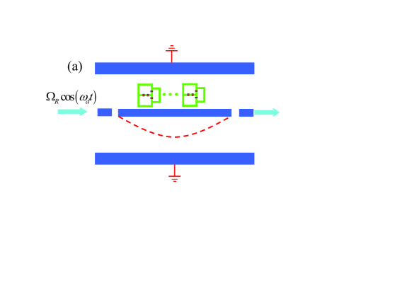
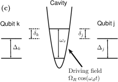
Figure 1: Schematic description of our setup. (a) The flux qubits are placed around current anti-node of the TLR (half wavelength or full wavelength). The red dashed curve illustrates the amplitude of the magnetic field of the half-wavelength TLR. (b) Schematic description of the tunable gap gradiometric flux qubits. The crosses denote Josephson junctions. The qubit is controlled by the bias lines $I_{\varepsilon}$ and $I_{\alpha}$. (c) Energy-level diagram of the system. $\Delta,\omega_{d},\omega_{r}$ are energy gap of the qubits, driving microwave frequency, and fundamental frequency of the cavity mode, respectively. The strong classical driving field denoted by the large arrow resonantly interacts with the flux qubits. We assume that all qubits have the same Rabi frequency $\Omega_{R}$.

The investigated system is schematically shown in Fig. 1, where superconducting flux qubits are strongly coupled to a one-dimensional transmission line resonator (TLR) with the geometric length $L_{0}$, distributed inductor $L$, and capacitance $C$. We consider the fundamental mode of the TLR, which can be modeled as a simple harmonic oscillator with the Hamiltonian

$$H_{\rm TLR}=\omega_{r}a^{\dagger}a,$$ (1)

where we have set $\hbar=1$, the frequency of the fundamental mode is given by $\omega_{r}/2\pi=1/\sqrt{LC}$, $a^{\dagger}$ and $a$ are the creation and annihilation operators of the fundamental mode of the resonator.

As shown in Fig. 1(b), we assume that each flux qubit has a gradiometric configuration as studied in Ref. Paauw2009, . The gradiometric design is used to trap an odd number of fluxoids to bias the flux qubit at its optimal point, and also to greatly reduce environmental noise. In contrast to the flux qubit with three junctions, one of which has a critical current $\alpha$ times smaller than that of the two identical junctions, here the small $\alpha$-junction is replaced by a so-called $\alpha$-loop, formed by a SQUID with two identical Josephson junctions. In this case, the ratio $\alpha$ and thus the coupling strength $\Delta$ between two circulating current states can be tuned via the magnetic flux $f_{\alpha}\Phi_{0}$ through the SQUID loop, where $\Phi_{0}$ is the magnetic flux quantum. The flux qubit Hamiltonian can be written as

$$H_{qb}=-\frac{1}{2}[\varepsilon\bar{\sigma}_{z}+\Delta(f_{\alpha}\Phi_{0})\bar{\sigma}_{x}],$$ (2)

where the Pauli matrices read $\bar{\sigma}_{z}=|0\rangle\langle 0|-|1\rangle\langle 1|$ and $\bar{\sigma}_{x}=0\rangle\langle 1|+|1\rangle\langle 0|$, in which $|0\rangle$ and $|1\rangle$ are the clockwise and counterclockwise persistent current states. $\varepsilon(f_{\varepsilon},f_{\alpha})=2I_{p}f_{\varepsilon}\Phi_{0}$ is the biased magnetic energy where $I_{p}$ is the persistent current in the qubit and $f_{\varepsilon}=f_{1}-f_{2}$ is the magnetic frustration difference in the two loop halves of the gradiometer. The energy gap $\Delta(f_{\alpha}\Phi_{0})$ can be controlled through the external magnetic flux $f_{\alpha}\Phi_{0}$.

Let us now assume that the flux qubits are placed around the current anti-node of the TLR. The coupling between qubits and the TLR is approximately homogeneous because the dimension of the qubits is on the order of several micrometers, which is much smaller than the wavelength of a few centimeters for the fundamental electromagnetic modes in microwave frequency regime. We also assume that the distance between the two nearest flux qubits is sufficiently large ($\sim 80\,\mu m$) to ensure that there are no direct interaction between different qubits. The coupling strength between the $k$-th flux qubit and the TLR is given as $g_{k}=M_{k}I_{p}^{k}I_{r0}$, where $M_{k}$ is the mutual inductance between the qubit and the resonator, $I_{r0}=\sqrt{\hbar\omega_{r}/L}$ is the zero-point current in the resonator.

The flux qubits are assumed to be near the optimal point ($\varepsilon\approx 0$), and thus the total system Hamiltonian is as follows (refer to see Appendix A for detailed derivations):

$$H_{s}=H_{0}+H_{I}+H_{d},$$ (3)

with

$$H_{0}=\omega_{r}a^{\dagger}a+\sum\limits_{k=1}^{N}\frac{\Delta_{k}}{2}\bar{\sigma}_{x}^{k},$$ (4)

$$H_{I}=\sum\limits_{k=1}^{N}g_{k}(a^{+}+a)\bar{\sigma}_{z}^{k},$$ (5)

$$H_{d}=\sum\limits_{k=1}^{N}\Omega_{R}\cos(\omega_{d}t)\,\bar{\sigma}_{z}^{k}.$$ (6)

Here, $H_{0}$ is the free Hamiltonian of the qubits and the cavity mode, $H_{I}$ is the interaction Hamiltonian between the qubits and the cavity mode, and $H_{d}$ describes the interaction between the qubits and classical driving microwave field. We assume that all qubits have the same frequency $\omega_{d}$ of the driving microwave field and the same Rabi frequency $\Omega_{R}$. It should be noted here that the homogenous coupling $\Omega_{R}$ is induced by the classical field that is applied to the TLR (see Appendix A).

In the basis of the eigenstates of the qubits and neglecting fast oscillating terms using the rotating-wave approximation (RWA) if $g_{k}\ll\omega_{r}$ and $\Omega_{R}\ll\omega_{d}$, the Hamiltonian in Eq. (3) takes the form

$$\widetilde{H_{1}} = \omega_{r}a^{+}a+\sum\limits_{k=1}^{N}\frac{\Delta_{k}}{2}\sigma_{z}^{k}+\sum\limits_{k=1}^{N}g_{k}(a^{+}\sigma_{-}^{k}+a\sigma_{+}^{k})$$ (7)

$$+ \sum\limits_{k=1}^{N}\frac{\Omega_{R}}{2}(\sigma_{+}^{k}e^{-i\omega_{d}t}+\sigma_{-}^{k}e^{i\omega_{d}t}).$$

Because the energy gap $\Delta_{k}$ for each qubit can be tuned by the biased flux in the $\alpha$ loop, without loss of generality, we assume the energy gap of flux qubits are equal, i.e., $\Delta_{k}\equiv\Delta$. Thus, in the rotating reference frame at the frequency $\omega_{d}=\Delta$, the Hamiltonian in Eq. (7) is changed to

$$\widetilde{H_{2}}=\delta\,a^{+}a+\sum\limits_{k=1}^{N}g_{k}(a^{+}\sigma_{-}^{k}+a\sigma_{+}^{k})+\sum\limits_{k=1}^{N}\frac{\Omega_{R}}{2}(\sigma_{+}^{k}+\sigma_{-}^{k}),$$ (8)

where we have defined the detuning $\delta=\omega_{r}-\omega_{d}>0$ between the cavity field and the driving field, and the ladder operators $\sigma_{+}=|-\rangle\langle+|$ and $\sigma_{-}=|+\rangle\langle-|$ by using ground $|+\rangle$ and first exited $|-\rangle$ states of qubits. (If $\delta<0$, it only means the transition frequency of flux qubits is larger than the frequency of the fundamental cavity mode and also works well in our scheme.) Here, we assume that the circuit QED system works in small detuning regime, i.e., $\delta>g_{k}$ (not $\delta\gg g_{k}$). The third term of the Hamiltonian in Eq. (8) implies the free Hamiltonian of the dressed qubits by the driving field liu-2006 .

In the interaction picture with the unitary transformation

$$U(t)=\exp(-iH_{\rm fr}t)$$ (9)

for the free Hamiltonian

$$H_{\rm fr}=\delta a^{+}a+\sum\limits_{k=1}^{N}\frac{\Omega_{R}}{2}(\sigma_{+}^{k}+\sigma_{-}^{k}),$$

the interaction part of the Hamiltonian in Eq. (8)

$$H_{\rm int}=\sum\limits_{k=1}^{N}g_{k}(a^{+}\sigma_{-}^{k}+a\sigma_{+}^{k}).$$

becomes

$$\widetilde{H_{3}} = U^{\dagger}(t)H_{\rm int}U(t)$$ (10)

$$= \sum\limits_{k=1}^{N}\frac{g_{k}}{2}\{e^{-i\delta t}a[\sigma_{x}^{k}+\frac{1}{2}(\sigma_{z}^{k}-i\sigma_{y}^{k})e^{i\Omega_{R}t}$$

$$-\frac{1}{2}(\sigma_{z}^{k}+i\sigma_{y}^{k})e^{-i\Omega_{R}t}]\}+H.c.$$

In the strong-driving regime, i.e., $\Omega_{R}\gg\delta,\,g_{k}$, we can neglect fast oscillating terms and the Hamiltonian in Eq. (10) turns into

$$H_{\rm eff} = \sum\limits_{k=1}^{N}\frac{g_{k}}{2}\sigma_{x}^{k}\{ae^{-i\delta t}+a^{\dagger}e^{i\delta t}\}.$$ (11)

The time evolution operator for the Hamiltonian in Eq. (11) can be written Wei1963 ; wang2001 as

$$U(t) = \prod\limits_{k\neq j}^{N}\exp\left\{-\int_{0}^{t}B_{k}^{*}(t)dB_{k}(t)\sigma_{x}^{k}\sigma_{x}^{j}\right\}$$

$$\prod\limits_{k}^{N}\exp\{-iB_{k}^{*}(t)a\sigma_{x}^{k}\}\prod\limits_{k}^{N}\exp\{-iB_{k}(t)a^{+}\sigma_{x}^{k}\},$$

with

$$B_{k}(t)=\frac{ig_{k}}{2\delta}(e^{i\delta t}-1).$$ (13)

It is obvious that $B_{k}(t)$ is a periodic function and vanishes at $t=T_{n}=2n\pi/\delta$ with the integer $n$. At these times, $U(t)$ is independent of the variables of the cavity field and the flux qubits are decoupled from cavity field. We define

$$\gamma_{kj}(t)\equiv\frac{1}{i}\int_{0}^{t}B_{k}^{*}(t)dB_{j}(t)=\frac{g_{k}g_{j}}{4\delta}\left[t-\frac{1}{i\delta}\left(e^{i\delta t}-1\right)\right].$$ (14)

At time $T_{n}$, the time evolution operator takes the form

$$U(T_{n},\gamma_{kj}) = \exp\left(-i\sum\limits_{k\neq j}^{N}\gamma_{kj}(T_{n})\sigma_{x}^{k}\sigma_{x}^{j}\right)$$ (15)

$$= \exp\left(-i\sum\limits_{k\neq j}^{N}\frac{n\pi g_{k}g_{j}}{2\delta^{2}}\sigma_{x}^{k}\sigma_{x}^{j}\right).$$

For the convenience of the discussions, let us now assume that the qubits are equally coupled to the resonator, i.e., $g_{k}=g_{j}\equiv g$, and thus we assume $\gamma_{kj}\equiv\gamma$. It should be noticed that the inhomogenous coupling is not a significant problem in our scheme. Actually, the homogenous coupling is not really required for this type of gate. The extra phase resulted from the inhomogenous coupling can be easily corrected by single qubit operations as mentioned in experiments Leibfried2003 . If we adjust the parameters such that $\gamma=(1+2m)\pi/8$ with an arbitrary integer $m$, then the initially unentangled state $|\psi(0)\rangle=\otimes_{k=1}^{N}|+\rangle_{k}$ can be changed to the GHZ state with the unitary evolution $U(\gamma)$, here $|\pm\rangle=(|0\rangle\pm|1\rangle)/\sqrt{2}$. The parameter $\gamma$ is a geometric phase which will be addressed elsewhere. If the parameters are selected as $n=1$, $m=0$, $g_{k}=2\pi\times 50$ MHz, $\delta=2g_{k}$, then the GHZ state

$$|{\rm GHZ}\rangle=\frac{1}{\sqrt{2}}\left(\bigotimes\limits_{k=1}^{N}|+\rangle_{k}+e^{i\pi(N+1)/2}\bigotimes\limits_{k=1}^{N}|-\rangle_{k}\right)$$ (16)

is produced at the time $T=10$ ns. We notice that there are two theoretical works on realization of controlled phase gate based on the $\gamma$ with superconducting qubits Yang2010 ; Wu2010 .

II.2 Numerical Simulation

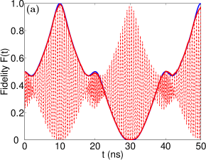
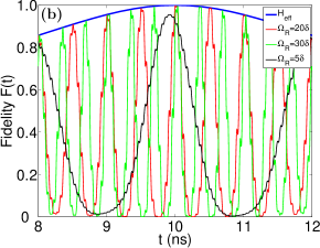
Figure 2: Time dependence of the fidelity of the generated entangled state in two flux qubits coupled to one TLR. The following parameters were used: $\omega_{r}=2\pi\times$10 GHz, $\Delta=2\pi\times 10.1\,$GHz, $g=2\pi\times 50\,$MHz, $\delta=-2\pi\times 100\,$MHz. The target EPR state is $(|++\rangle+i|--\rangle)/\sqrt{2}$. (a) The blue solid, red solid, and red dashed curves are simulated using the effective Hamiltonians in Eq. (11) and in Eq. (10) and the full Hamiltonian in Eq. (II.2), respectively, with the optimized driving strength $\Omega=20\delta$. (b) Simulation using the full Hamiltonian in Eq. (II.2) for different driving strengths around the time $t=2\pi/\delta=10\,$ns.

To verify the validity of the approach proposed here, we now present numerical calculations. We simulate the dynamics of the system by using both its full Hamiltonian in Eq. (3) without making any approximation, and the effective Hamiltonians in Eqs. (10) and (11). For the convenience, we can rewrite the full Hamiltonian in Eq. (3), in the basis of the eigenstates of the qubits and the rotating reference frame of $\omega_{d}$, as

$$\widetilde{H}_{\rm s} = \widetilde{H_{2}}+\sum\limits_{k=1}^{N}\frac{\Omega_{R}}{2}(\sigma_{+}^{k}e^{2i\omega_{d}t}+\sigma_{-}^{k}e^{-2i\omega_{d}t})$$

$$+ \sum\limits_{k=1}^{N}g_{k}(a^{+}\sigma_{+}^{k}e^{i(\omega_{r}+\omega_{d})t}+a\sigma_{-}^{k}e^{-i(\omega_{r}+\omega_{d})t}).$$

Let us assume that the cavity field is initially in the vacuum state $|0\rangle_{c}$, and the $k$-th qubit is initially in the state $|+\rangle_{k}=(|0\rangle+|1\rangle)/\sqrt{2}$, that is, the initial state of the whole system is

$$|\psi(0)\rangle=\bigotimes_{k=1}^{N}|+\rangle_{k}|0\rangle_{c}=\bigotimes_{k=1}^{N}\frac{1}{\sqrt{2}}\left(|0\rangle_{k}+|1\rangle_{k}\right)|0\rangle_{c}.$$ (18)

We can solve the Schrödinger equation to obtain the state $|\psi(t)\rangle$ at any time by using the Hamiltonians in Eq. (10), Eq. (11) and Eq. (II.2). Then we compare these states $|\psi(t)\rangle$ with the expected ideal GHZ state by using the fidelity

$$F(t)=Tr[\rho_{\rm GHZ}\rho_{q}(t)],$$ (19)

where $\rho_{q}(t)$ is the reduced density matrix of the $N$ qubits and $\rho_{\rm GHZ}$ is the density matrix of the $N$-qubit GHZ state.

As an example, let us consider the interaction between two qubits and the cavity field with the initial state $|++\rangle|0\rangle_{c}$. In Fig. 2, the fidelities $F(t)$ of different outcomes versus the evolution time $t$ are plotted. In Fig. 2(a), we find that both the full Hamiltonian in Eq. (II.2) and the effective Hamiltonians in either Eq. (10) or Eq. (11) well describe the dynamics of the two-qubits system. The expected entangled state $(|++\rangle+i|--\rangle)/\sqrt{2}$ can be generated in $t=10$ ns, which is comparable with the single-qubit operation time.

To illustrate how the driving strength affects the fidelity of the expected GHZ state, we plot Fig. 2(b) by using the Hamiltonian in Eq. (II.2) for different driving strengths. It can be clearly seen that the counter-rotating term of the driving field becomes important and reduces the fidelity when the driving strength is too strong. On the other hand, if the driving is too weak and the condition $\Omega_{R}\gg{g_{k},\delta}$ is not met any more, the fast oscillating terms in Eq. (10) must be taken into account. Therefore, the driving field has to be optimized so that the maximum fidelity can be achieved. We provide a more detailed analysis of the effect of these fast oscillating terms on the fidelity of the generated state below. With the optimized driving strength, the fidelity is at best above $99.5\%$. It should be noted here that we did not make an adiabatic approximation for the fast variable $\Omega_{R}$ in our simulation. Therefore, to prepare high fidelity GHZ states, the accuracy of control of the microwave pulse time should be determined by $2\pi/\Omega_{R}$ in our scheme from analysis of the full system Hamiltonian. For example, to realize the preparation with a fidelity exceeding $90\%$, the precision of the microwave pulse time should be around $100\,$ps for the detuning $\delta=-2\pi\times 100\,$MHz and $\Omega_{R}=2\pi\times 2\,$GHz in Fig. 2(b). This is easily realized with a commercial pulse generator having a precision of $10\,$ps.

In Ref. Wang2010, , to increase the effective coupling between qubits, they have to increase $g$ (the coupling strength between qubits and resonator) and decrease the resonator frequency $\omega_{r}$. We argue that it is valid in experiments to make an adiabatic approximation for the resonator frequency $\omega_{r}$ when $g$ is approaching $\omega_{r}$ as in Fig. 2 of Ref. Wang2010, . Otherwise, to prepare high fidelity GHZ states in their scheme, the accuracy of control of the dc current pulse time is determined by $2\pi/\omega_{r}$, not by $2\pi\omega_{r}/g^{2}$. It means that the accuracy must be on the order of a few hundred ps for the selected parameters $\omega_{r}=2\pi\times 1\,$GHz and $g=2\pi\times 144\,$MHz in Fig. 2 of Ref. Wang2010, . Such accuracy would present a major challenge for state-of-the-art dc current pulse technology.

II.3 Nonideal Case

In the derivation of effective Hamiltonian in Eq. (10), we have neglected the following terms

$$H_{n} = \sum\limits_{k=1}^{N}\frac{g_{k}}{4}\left\{\left[(\sigma_{z}^{k}-i\sigma_{y}^{k})e^{i\Omega_{R}t}\right.\right.$$

$$- \left.\left.(\sigma_{z}^{k}+i\sigma_{y}^{k})e^{-i\Omega_{R}t}\right]ae^{-i\delta t}+H.c.\right\}$$

$$= \sum\limits_{k=1}^{N}\frac{ig_{k}}{2}\left[\sin(\Omega_{R}t)\sigma_{z}^{k}-\cos(\Omega_{R}t)\sigma_{y}^{k}\right]ae^{-i\delta t}+H.c.\,.$$

These terms could reduce the fidelity of the gate. However, we can use the spin-echo technique to eliminate the errors from the $\sigma_{z}$ terms. Below, we will only study the effect of the $\sigma_{y}$ terms on the gate operation using the method described in Ref. Sorensen2000, .

In the interaction picture, the interaction Hamiltonian is $H_{n,I}(t)=U^{\dagger}(t)H_{n}(t)U(t)$, and we have the propagator $U_{I}(t)$ from the Dyson series,

$$U_{I}(t) = 1-i\int_{0}^{t}dt^{\prime}H_{n,I}(t^{\prime})$$ (21)

$$-\int_{0}^{t}\int_{0}^{t^{\prime}}dt^{\prime}dt^{\prime\prime}H_{n,I}(t^{\prime})H_{n,I}(t^{\prime\prime})+\cdots.$$

We can treat $U(t)$ as a constant during the integration because $H_{n}(t)$ is oscillating much faster than the propagator. Then, we get

$$U_{I}(t) = 1-\frac{g}{2\Omega_{R}}\sin(\Omega_{R}t)\sum\limits_{k=1}^{N}\{U^{\dagger}(t)\sigma_{y}^{k}U(t)\}$$ (22)

$$+i\frac{g^{2}}{4\Omega_{R}^{2}}\sum\limits_{k\neq j}^{N}\{(1-\cos(2\Omega_{R}t))U^{\dagger}(t)\sigma_{y}^{k}\sigma_{y}^{j}U(t)\}$$

$$+\cdots.$$

Near the time $t=2\pi n/\delta$, $U(t)\approx\exp(-i\sum\limits_{k\neq j}^{N}\gamma\sigma_{x}^{k}\sigma_{x}^{j})$ and we obtain the fidelity

$$F(t)\approx 1-\frac{N(N-1)g^{2}}{8\Omega_{R}^{2}}(1-\cos(2\Omega_{R}t)),$$ (23)

where $N$ is the number of qubits involved in the gate. It should be noted that the estimation of $F(t)$ is obtained in the interaction picture. In the rotating frame and near the time $t=2\pi n/\delta$, the time evolution operator takes the form

$$\widetilde{U}(t)\approx\exp(-i\sum\limits_{k}^{N}\Omega_{R}t\sigma_{x}^{k}/2)\exp(-i\sum\limits_{k\neq j}^{N}\gamma\sigma_{x}^{k}\sigma_{x}^{j}).$$ (24)

In the experiment, we can accurately control the duration of classical microwave field to fulfill the condition both $\delta t=2n\pi$ and $\Omega_{R}t=4n^{\prime}\pi$ ($n$ and $n^{\prime}$ are arbitrary integers) so that the effect of the $\sigma_{y}$ terms and $\exp(-i\sum\limits_{k}^{N}\Omega_{R}t\sigma_{x}^{k}/2)$ vanishes. When $N$ is not too large, e.g., $N<\Omega_{r}/g$, $F(t)$ is mainly limited by the accuracy of control of the microwave pulse. On the other hand, if the accuracy of control of the microwave pulse is fixed, there is a polynomial decrease of the fidelity according to $N$.

Our scheme works in the strong-driving regime, i.e., $\Omega_{R}\gg\delta,g_{k}$, so we can select the optimized driving strength $\Omega_{R}=20\delta=40g$ from the numerical simulation in Fig. 2(b) and use Eq. (23) and Eq. (24) to roughly estimate the fidelity of the generated multi-particle GHZ state. In this case, $F(t)\sim 1$ near the time $t=2\pi/\delta=10\,$ns for $N<40$. We can conservatively expect that our one-step proposal will work well for more than 20 qubits are placed at the current anti-node of the resonator by considering the inhomogenous coupling between qubits and resonator.

III Scalable circuit with tunable TLRs and tunable nodes

III.1 Scalable model

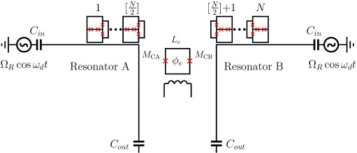
Figure 3: Schematic description of flux qubits coupled to two tunably coupled TLRs (half-wavelength TLRs or full-wavelength TLRs). $N$ qubits are coupled to the current anti-node of the two resonators. A dc-SQUID is placed at the current anti-node of the two resonators. The inductive coupling between two resonators could be tuned by changing the biased flux $\phi_{e}$ in the symmetric dc-SQUID loop. Two classical microwave fields resonantly interact with $N$ qubits by driving the TLRs. $L_{c}$, $M_{\rm CA}$, $M_{\rm CB}$ are self-inductance of the dc-SQUID coupler loop, mutual inductance between the coupler and Resonator A, and mutual inductance between the coupler and Resonator B, respectively.

In our design, the half wavelength of the TLR for the fundamental mode frequency $\omega_{r}=2\pi\times 10$ GHz is around $6$ mm Abdumalikov2008 . If the distance between the two nearest flux qubits is around $80$ $\mu$m, we can only place about $6$ flux qubits around the current anti-node position where the current variation is about $0.5\%$. Although the electric field is not completely zero around the anti-node, its effect on flux qubits is negligibly small. It is possible to place more than 6 flux qubits in the half wavelength TLR because we can, in principle, design the coupling inductance so that the coupling constant $g_{k}$ is uniform in a wider range around the current anti-node. If there are extra phases arising from inhomogenous coupling between the qubits and TLR, we can correct them with additional single-qubit operations.

Here, we study the one-step generation of high-fidelity GHZ states for many qubits. We did not select a longer resonator with a low frequency of the fundamental cavity mode to solve the problem of the scalability, for the following two reasons. First, the lower frequency of the fundamental cavity mode may lead to more operational errors resulting from the thermal excitations in the cavity. Second, the derived effective Hamiltonian in Eq. (11) is valid in the strong-driving regime. If the driving strength in units of Rabi frequency approaches the energy gap of qubits, the counter-wave terms have to be taken into account, as shown in Fig. 2(b).

To solve the problem of the scalability, let us now use two coupled TLRs as an example to show how the multiparticle GHZ state can be generated via several TLRs in one step. As shown in Fig. 3, $N$ qubits are placed into two cavities formed by two TRLs coupled by a symmetric dc-SQUID. We assume that the qubits labeled from $1$ to $[N/2]$ interacted with TRL A, and other qubits labeled from $[N/2]$ to $N$ are coupled to TRL B, where $[N/2]$ means the maximum integer no more than $N/2$. Near the optimal point and in the basis of the flux qubit persistent current states, the total system Hamiltonian can be given as

$$H_{s}^{\prime} = \omega_{a}a^{\dagger}a+\sum\limits_{k=1}^{[\frac{N}{2}]}\frac{\Delta_{k}}{2}\bar{\sigma}_{x}^{k}+\sum\limits_{k=1}^{[\frac{N}{2}]}g_{k}\bar{\sigma}_{z}^{k}(a^{\dagger}+a)$$ (25)

$$+\omega_{b}b^{\dagger}b+\sum\limits_{j=[\frac{N}{2}]+1}^{N}\frac{\Delta_{j}}{2}\bar{\sigma}_{x}^{j}+\sum\limits_{j=[\frac{N}{2}]+1}^{N}g_{j}\bar{\sigma}_{z}^{j}(b^{\dagger}+b)$$

$$+J(\phi_{e})(a^{\dagger}b+ab^{\dagger})+\sum\limits_{k=1}^{N}\Omega_{R}\cos(\omega_{d}t)\bar{\sigma}_{z}^{k}.$$

Here, the operators $a(a^{\dagger})$ and $b(b^{\dagger})$ are annihilation (creation) operators for the field in cavity A with the frequency $\omega_{a}$ and cavity B with the frequency $\omega_{b}$, respectively. $g_{k}$ is the coupling constant between the $k$-th qubit and the TRL $A$, and $g_{j}$ denotes the coupling of the $j$-th qubit and the TRL $B$.

The parameter $J(\phi_{e})=M_{\rm eff}(\phi_{e})I_{\rm A0}I_{\rm B0}$ is the inductive coupling constant between two TRLs, where $I_{\rm A0}$, $I_{\rm B0}$ are the zero point current in cavity A and cavity B, respectively. It is possible to tune $M_{\rm eff}$ by changing the penetrated flux $\phi_{e}$ in the dc-SQUID loop, given by Brink2005

$$M_{\rm eff}(\phi_{e}) = -\dfrac{M_{\rm CA}M_{\rm CB}}{L_{c}}\dfrac{\beta_{L}\cos(l\pi-\pi\dfrac{\phi_{e}}{\Phi_{0}})}{2+\beta_{L}\cos(l\pi-\pi\dfrac{\phi_{e}}{\Phi_{0}})},$$ (26)

where $l$ is an arbitrary integer, $I_{c}$ is the critical current of the two identical Josephson junctions in the dc-SQUID, and screening parameter $\beta_{L}\equiv 2\pi L_{c}I_{c}/\Phi_{0}<1$ to ensure that the coupler works in the nonhysteretic regime. We have ignored the direct inductive coupling between two resonators. More detailed discussions of the dc-SQUID coupler can be found in Refs. Brink2005, and Plourde2004, .

We assume that all qubits are equally driven by the classical field with the frequency $\omega_{d}$, and the coupling between the qubits and the driving field is characterized by the constant $\Omega_{R}$. We rewrite the Hamiltonian in Eq. (25) in the basis of the qubit eigenstates and make the rotating wave approximation, thus the Hamiltonian in Eq. (25) becomes

$$\widetilde{H_{1}}^{\prime} = \omega_{a}a^{\dagger}a+\sum\limits_{k=1}^{[\frac{N}{2}]}\frac{\Delta_{k}}{2}\sigma_{z}^{k}+\sum\limits_{k=1}^{[\frac{N}{2}]}g_{k}(\sigma_{-}^{k}a^{\dagger}+H.c.)$$

$$+\omega_{b}b^{\dagger}b+\sum\limits_{j=[\frac{N}{2}]+1}^{N}\frac{\Delta_{j}}{2}\sigma_{z}^{j}+\sum\limits_{j=[\frac{N}{2}]+1}^{N}g_{j}(\sigma_{-}^{j}b^{\dagger}+H.c.)$$

$$+J(\phi_{e})(a^{\dagger}b+ab^{\dagger})+\sum\limits_{k=1}^{N}\frac{\Omega_{R}}{2}(\sigma_{+}^{k}e^{-i\omega_{d}t}+H.c.).$$

Without loss of generality, in the following discussion we assume $\omega_{a}=\omega_{b}=\omega$, which can be experimentally achieved. Because the TLR is a distributed element, we can easily design its fundamental mode frequency in experiments. Now we introduce a canonical transformation to Eq. (III.1) via the operators

$$P = \frac{1}{\sqrt{2}}(a+b),$$

$$Q = \frac{1}{\sqrt{2}}(a-b).$$ (28)

Since the operators $a$ and $b$ describe different cavity fields in the different cavities, they satisfy the condition $[a,\,b]=0$ and then $[P,\,Q]=0$. Substituting Eq. (III.1) into Eq. (III.1) and in the rotating reference frame of the resonant frequency $\omega_{d}=\Delta$, we have

$$\widetilde{H_{2}}^{\prime} = (\omega+J)P^{\dagger}P+\frac{1}{\sqrt{2}}\sum\limits_{k=1}^{[N/2]}g_{k}(\sigma_{-}^{k}P^{\dagger}+\sigma_{+}^{k}P)$$

$$+\frac{1}{\sqrt{2}}\sum\limits_{j=[N/2]+1}^{N}g_{j}(\sigma_{-}^{j}P^{\dagger}+\sigma_{+}^{j}P)$$

$$+(\omega-J)Q^{\dagger}Q+\frac{1}{\sqrt{2}}\sum\limits_{k=1}^{[N/2]}g_{k}(\sigma_{-}^{k}Q^{\dagger}+\sigma_{+}^{k}Q)$$

$$-\frac{1}{\sqrt{2}}\sum\limits_{j=[N/2]+1}^{N}g_{j}(\sigma_{-}^{j}Q^{\dagger}+\sigma_{+}^{j}Q)+\sum\limits_{k=1}^{N}\frac{\Omega_{R}}{2}\sigma_{x}^{k}.$$

Using the same method as for the derivation of the effective Hamiltonian in Eq. (11) for the flux qubits coupled to a TLR, based on Eq. (III.1), we can derive an effective Hamiltonian for the qubits coupled to two TRLs as

$$H_{\rm eff}^{\prime} = \sum\limits_{k=1}^{[N/2]}\frac{\sqrt{2}}{4}g_{k}\sigma_{x}^{k}\left({Pe^{-i(\delta^{\prime}+J)t}+P^{\dagger}e^{i(\delta^{\prime}+J)t}}\right)$$

$$+\sum\limits_{j=[N/2]+1}^{N}\frac{\sqrt{2}}{4}g_{j}\sigma_{x}^{j}\left({Pe^{-i(\delta^{\prime}+J)t}+P^{\dagger}e^{i(\delta^{\prime}+J)t}}\right)$$

$$+\sum\limits_{k=1}^{[N/2]}\frac{\sqrt{2}}{4}g_{k}\sigma_{x}^{k}\left({Qe^{-i(\delta^{\prime}-J)t}+Q^{\dagger}e^{i(\delta^{\prime}-J)t}}\right)$$

$$-\sum\limits_{j=[N/2]+1}^{N}\frac{\sqrt{2}}{4}g_{j}\sigma_{x}^{j}\left({Qe^{-i(\delta^{\prime}-J)t}+Q^{\dagger}e^{i(\delta^{\prime}-J)t}}\right),$$

with $\delta^{\prime}=\omega-\omega_{d}$. Here, we already neglect fast oscillating terms under the strong driving condition $\Omega_{R}\gg g_{k},\,\delta^{\prime},J$.

When $\delta^{\prime}>J,\,g_{k}$, and $\delta^{\prime}=\xi J\,$( $\xi$ is an arbitrary odd integer), at the time $t=T_{n}=2\pi n/J$, the flux qubits are decoupled from resonators. In this case, we have

$$\sum\limits_{k\neq j}^{N}\gamma_{kj}(T_{n}) = \frac{1}{4}\left[\sum\limits_{k,j=1;k\neq j}^{[N/2]}\frac{g_{k}g_{j}}{(\delta^{\prime}+J)(\delta^{\prime}-J)}\delta^{\prime}\right.$$

$$+\sum\limits_{k,j=[\frac{N}{2}+1];k\neq j}^{N}\frac{g_{k}g_{j}}{(\delta^{\prime}+J)(\delta^{\prime}-J)}\delta^{\prime}$$

$$\left.-\sum\limits_{k=1}^{[N/2]}\sum\limits_{j=[\frac{N}{2}]+1}^{N}\frac{g_{k}g_{j}}{(\delta^{\prime}+J)(\delta^{\prime}-J)}J\right]\cdot T_{n}.$$

In the above equation, the first and second terms show that the flux qubits coupled to the same resonator are in permutation symmetry. The third term shows that the coupling between any two qubits mediated by the two coupled TLRs is weaker than the first two terms, and there is also a sign difference between the first two terms and the third term. If we adjust the detuning $\delta^{\prime}$ and the coupling constant $J(\phi_{e})$ such that the conditions

$$\frac{g_{k}g_{j}}{(\delta^{\prime}+J)(\delta^{\prime}-J)}\delta^{\prime}\cdot T_{n}=\frac{1}{2}(3+4m)\pi$$ (32)

and

$$\frac{g_{k}g_{j}}{(\delta^{\prime}+J)(\delta^{\prime}-J)}J\cdot T_{n}=\frac{1}{2}(1+4l)\pi$$ (33)

are satisfied simultaneously, where $l$ and $m$ are arbitrary integers, then the multiple particle GHZ state can be generated in one step. If we chose $n=1$, $m=l=0$, $J=2\pi\times 40$ MHz, $g_{k}=\sqrt{2}J$ ($k=1\cdots N$), $\delta^{\prime}=-3J=-2\pi\times 120$ MHz, the GHZ state can generated in $25$ ns. We would like to emphasize that $J=2\pi\times 40\,$MHz is a reasonable value in experiments. If we assume $I_{\rm Ar0}=I_{\rm Br0}=50$ nA, $J=2\pi\times 40\,$MHz means that the effective mutual inductance $M_{\rm eff}$ between two TLRs mediated by dc-SQUID is around $5.32$ pH. It is experimentally realizable with the selected parameters as $I_{c}=1.5\,\mu$A, $M_{\rm CA}=M_{\rm CB}=60\,$pH and $L_{c}=200\,$pH for the dc-SQUID coupler. It is possible to continuously tune the coupling from anti-ferromagnetic to ferromagnetic like a rf-SQUID coupler in experiments Allman2010 . We notice that there is a theoretical work on a flux qubit mediating the coupling between two TLRs and working as a quantum switch Mariantoni2008 . In that scheme, it is also possible to realize tunable coupling between two TLRs mediated by the flux qubit.

Now, we consider how to generate $N$-qubit ($N>20$) GHZ states in one step. As shown in Fig. 4, a dc-SQUID coupler is coupled to $M$ TLRs which form a circle array. Flux qubits are placed at current anti-nodes of the TLRs. For the convenience of discussions, we assume that the coupling constants between resonators and the center coupler are homogenous. The resonators are in permutation symmetry. If we select parameters to simultaneously meet conditions such as those in Eq. (32) and Eq. (33), we can, in principle, extend our scheme to the case of many qubits.

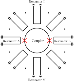
Figure 4: Schematic description of a circle array of TLRs coupled by a dc-SQUID. $M$ TLRs are placed as the current anti-nodes around the coupler. Flux qubits are coupled to the current anti-nodes of the TLRs.

III.2 Numerical Simulation

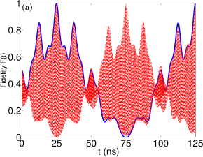
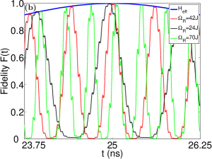
Figure 5: Time dependence of the fidelity of the generated entangled state for two flux qubits which are coupled by two coupled TLRs. Here, the two qubits are separately coupled to the two TRLs. We set the following parameters for our numerical calculations: $\omega_{r}=2\pi\times 10$ GHz, $\Delta=2\pi\times 10.12$ GHz, $J=2\pi\times 40$ MHz, $g_{k}=\sqrt{2}J$ and $\delta^{\prime}=-3J$. The target state is $(|++\rangle+i|--\rangle)/\sqrt{2}$. (a) The blue solid and red dashed curves are simulated using the effective Hamiltonian Eq. (III.1) and the full Hamiltonian in Eq. (III.2), respectively, with optimized driving strength $\Omega_{R}=42J$. (b) Simulation using the full Hamiltonian in Eq. (III.2) with different driving strengths around the time $t=2\pi/J=25\,$ns.

For flux qubits coupled to a system of two coupled TLRs, the numerical simulation procedure is similar to that in previous case. We can assume that all qubits are initially in the state $\otimes_{k=1}^{N}|+\rangle_{k}$ and that the two cavity fields are initially in the vacuum state $|00\rangle_{c}$, i.e., that the initial state of the whole system is $|\psi(0)\rangle=\otimes_{k=1}^{N}|+\rangle_{k}|00\rangle_{c}$. The full Hamiltonian used in the simulation is

$$H_{\rm full,sim}^{\prime} = \widetilde{H_{2}}^{\prime}+\sum\limits_{k=1}^{N}\frac{\Omega_{R}}{2}\left(\sigma_{+}^{k}e^{2i\omega_{d}t}+\sigma_{-}^{k}e^{-2i\omega_{d}t}\right)$$

$$+ \frac{1}{\sqrt{2}}g_{k}\sum\limits_{k=1}^{[N/2]}\left(P^{+}\sigma_{+}^{k}e^{i(\omega_{r}+\omega_{d})t}+H.c.\right)$$

$$+ \frac{1}{\sqrt{2}}g_{j}\sum\limits_{j=[N/2]+1}^{N}\left(P^{+}\sigma_{+}^{j}e^{i(\omega_{r}+\omega_{d})t}+H.c.\right)$$

$$+ \frac{1}{\sqrt{2}}g_{k}\sum\limits_{k=1}^{[N/2]}\left(Q^{+}\sigma_{+}^{k}e^{i(\omega_{r}+\omega_{d})t}+H.c.\right)$$

$$- \frac{1}{\sqrt{2}}g_{j}\sum\limits_{j=[N/2]+1}^{[N]}\left(Q^{+}\sigma_{+}^{j}e^{i(\omega_{r}+\omega_{d})t}+H.c.\right).$$

Comparing the simulation results shown in Fig. 5 with the full Hamiltonian and the effective Hamiltonian, we find that the effective Hamiltonian in Eq. (III.1) can also describe the dynamics of two qubits system well. With the optimized driving strength, the maximum fidelity can be above $99.8\%$. The two qubits entangled state $(|++\rangle+i|--\rangle)/\sqrt{2}$ can be produced in $t=2\pi/J=25$ ns. Our proposal provides an obvious advantage in that the multiparticle GHZ states are generated in one step in $\sim 25$ ns with high fidelity. In contrast, in the experiments described in Refs. Neeley2010, and DiCarlo2010, , three-qubit GHZ state was generated step by step and the total generation time was $\sim 80$ ns with a fidelity of $\sim 90\%$. According to those experiments, the total generation time will linearly increase with the numbers of qubits.

IV Discussion and Summary

Let us now discuss the experimental feasibility. For a TLR with the fundamental mode frequency $\omega_{r}=2\pi\times 10$ GHz and the quality factor $Q\sim 10^{4}$, the decay rate is about $\sim 1$ MHz. The decoherence time achieved in the tunable gap gradiometric qubit is longer than $1\,\mu$s in experiments Fedorov2010 . Thus the GHZ state can be generated in about $10$ ns, which is much shorter than the decoherence time of qubits and the decay time in the TLR.

To demonstrate the GHZ state, we could use the well developed quantum state tomography technique in superconducting qubits liu-2005 to reconstruct the density matrix of the final state DiCarlo2010 ; Filipp2009 . After the GHZ state is generated, we can tune the transition frequencies of the qubits such that the interactions between all qubits and the TLRs are switched off. For example, the change of detuning from $2\pi\times 100$ MHz up to $2\pi\times 2$ GHz reduces the coupling strength by a factor of $20$. It is sufficient for experimental demonstration of the GHZ state using quantum state tomography.

We derive the effective Hamiltonian under the strong-driving condition. The strong driving on the flux qubit as high as $2\pi\times 2$ GHz has been realized in our group. A detailed theoretical analysis of leakage to higher energy levels under strongly resonant microwave driving is given in Ref. Ferron2010, . From these calculation, we can conclude that the leakage to higher energy levels is negligibly small because of the strong anharmonicity for flux qubits at the optimal point ($\varepsilon\approx 0$).

In summary, we have proposed a scheme for generation of the multiqubit GHZ entangled state in tunable gap flux qubits coupled to a TLR. We also extend this scheme to the case of tunable flux qubits coupled to two or more coupled TLRs. The operation time is comparable to that of the single-qubit operation. In principle, our proposal can be generalized to the case in which the tunable qubits are coupled to a circle array formed by $M$ coupled TLRs via a dc-SQUID coupler, that is, our proposal is scalable to some extent. We expect that our scheme has an useful contribution to the generation of cluster states for one-way quantum computation.

Appendix A Homogenous coupling between qubits and classical driving field through TLR

Let us now show how to obtain the Hamiltonian in Eq. (3) when the classical driving field is applied to the TRL. In our assumption, the driving microwave with large amplitude is substantially detuned from the frequency of resonator. In this situation, quantum fluctuation in the drive is very small compared to the drive amplitude, and the drive field could be considered as a classical field Blais2007 . The classical microwave field driving on the resonator can be described by

$$H_{D}=\nu(t)a^{+}e^{-i\omega_{d}t}+\nu^{*}(t)ae^{i\omega_{d}t}$$ (35)

where $\nu(t)$ is the amplitude and $\omega_{d}$ is the frequency of external driving. The Hamiltonian of the whole system is $H=H_{0}+H_{I}+H_{D}$, where $H_{0}$ in Eq. (4) and $H_{I}$ in Eq. (5). We can then displace the field operators using time dependent displacement operator

$$D(\beta)=\exp(\beta a^{+}-\beta^{*}a),$$ (36)

where $\beta$ is an arbitrary complex number and the field $a$ goes to $a+\beta$ under this unitary transformation.

In the case in which the driving amplitude $\varepsilon$ is independent of time, the displaced Hamiltonian in the energy eigenstate basis of qubits reads

$$\widetilde{H} = D^{+}(\beta)HD(\beta)-iD^{+}(\beta)\dot{D}(\beta)$$

$$= \omega_{r}a^{+}a+\frac{1}{2}\sum\limits_{k=1}^{N}\Delta_{k}\sigma_{z}^{k}+\sum\limits_{k=1}^{N}g_{k}[(a^{+}+\beta^{*})+(a+\beta)]\sigma_{x}^{k}$$

$$= \omega_{r}a^{+}a+\frac{1}{2}\sum\limits_{k=1}^{N}\Delta_{k}\sigma_{z}^{k}+\sum\limits_{k=1}^{N}g_{k}(a^{+}+a)\sigma_{x}^{k}+$$

$$\sum\limits_{k=1}^{N}\frac{2g_{k}\nu\cos(\omega_{d}t)}{\delta}\sigma_{x}^{k},$$

where $\beta(t)=\nu e^{-i\omega_{d}t}/\delta$, $\delta=\omega_{r}-\omega_{d}$.

The above Hamiltonian is the Hamiltonian in Eq. (3) in energy eigenstates basis of the qubits with $\Omega_{R}^{k}=2g_{k}\nu\cos(\omega_{d}t)/\delta$. If the qubits are equally coupled to the resonator, i.e., $g_{k}\equiv g$, we obtain homogenous coupling $\Omega_{R}$ between qubits and classical driving field through the TLR.

References

- (1) M. A. Nielsen and I. L. Chuang, Quantum Computation and Quantum Information (Cambridge University Press, Cambridge, 2000).
- (2) Y. Makhlin, G. Schön, and A. Shnirman, Rev. Mod. Phys. 73, 357 (2001).
- (3) J. Q. You and F. Nori, Nature 474, 589 (2011).
- (4) T. Monz, P. Schindler, J.T. Barreiro, M. Chwalla, D. Nigg, W.A. Coish, M. Harlander, W. Hänsel, M. Hennrich, and R. Blatt, Phys. Rev. Lett. 106, 130506 (2011).
- (5) W. B. Gao, C. Y. Lu, X. C. Yao, P. Xu, O. Gühne, A. Goebel, Y. A. Chen, C. Z. Peng, Z. B. Chen, J. W. Pan , Nature Phys. 6, 331 (2010).
- (6) L. F. Wei, Y. X. Liu, and F. Nori, Phys. Rev. Lett. 96, 246803 (2006).
- (7) M. D. Kim and S. Y. Cho, Phys. Rev. B 77, 100508 (2008).
- (8) A. Galiautdinov and J. M. Martinis, Phys. Rev. A 78, 010305 (2008).
- (9) A. J. Berkley, H. Xu, R. C. Ramos, M. A. Gubrud, F. W. Strauch, P. R. Johnson, J. R. Anderson, A. J. Dragt, C. J. Lobb, and F. C. Wellstood, Science 300, 1548 (2003).
- (10) A. Izmalkov, M. Grajcar, E. Il ichev, Th. Wagner, H.-G. Meyer, A. Yu. Smirnov, M. H. S. Amin, A. M. van den Brink, and A. M. Zagoskin, Phys. Rev. Lett. 93, 037003 (2004).
- (11) A. O. Niskanen, K. Harrabi, F. Yoshihara, Y. Nakamura, S. Lloyd, and J. S. Tsai, Science 316, 723 (2007).
- (12) J. H. Plantenberg, P. C. de Groot, C. J. P. M. Harmans, and J. E. Mooij, Nature 447, 836 (2007).
- (13) H. Xu, F. W. Strauch, S. K. Dutta, P. R. Johnson, R. C. Ramos, A. J. Berkley, H. Paik, J. R. Anderson, A. J. Dragt, C. J. Lobb, and F. C. Wellstood, Phys. Rev. Lett. 94, 027003 (2005).
- (14) M. Neeley, R. C. Bialczak, M. Lenander, E. Lucero, M. Mariantoni, A. D. O’Connell, D. Sank, H. Wang, M. Weides, J. Wenner, Y. Yin, T. Yamamoto, A. N. Cleland, and J. M. Martinis, Nature 467, 570 (2010).
- (15) L. DiCarlo, M. D. Reed, L. Sun, B. R. Johnson, J. M. Chow, J. M. Gambetta, L. Frunzio, S. M. Girvin, M. H. Devoret, and R. J. Schoelkopf, Nature 467, 574 (2010).
- (16) F. Altomare, J. I. Park, K. Cicak, M. A. Sillanpää, M. S. Allman, D. Li, A. Sirois, J. A. Strong, J. D. Whittaker, and R. W. Simmonds, Nature Phys. 6, 777 (2010).
- (17) A. Fedorov, L. Steffen, M. Baur, and A. Wallraff, arXiv:1108.3966 (2011).
- (18) R. J. Schoelkopf and S. M. Girvin, Nature 451, 664 (2008).
- (19) S.L. Zhu, Z.D. Wang, and P. Zanardi, Phys. Rev. Lett. 94, 100502 (2005).
- (20) F. Helmer and F. Marquardt, Phys. Rev. A 79, 052328 (2009).
- (21) L.S. Bishop, L. Tornberg, D. Price, E. Ginossar, A. Nunnen- kamp, A.A. Houck, J. M. Gambetta, J. Koch, G. Johansson, S.M. Girvin, and R. J. Schoelkopf, New J. Phys. 11, 073040 (2009).
- (22) C.L. Hutchison, J.M. Gambetta, A. Blais, and F.K. Wilhelm, Can. J. Phys. 87, 225 (2009).
- (23) D.I. Tsomokos, S. Ashhab, and F. Nori, New J. Phys. 10, 113020 (2008).
- (24) Y.D. Wang, S. Chesi, D. Loss, and C. Bruder, Phys. Rev. B 81, 104524 (2010).
- (25) K. Mølmer and A. Sørensen, Phys. Rev. Lett. 82, 1835 (1999).
- (26) A. Sørensen and K. Mølmer, Phys. Rev. A 62, 022311 (2000).
- (27) E. Solano, G.S. Agarwal, and H. Walther, Phys. Rev. Lett. 90, 027903 (2003).
- (28) S.B. Zheng, Phys. Rev. A 66, 060303(R) (2002).
- (29) F. G. Paauw, A. Fedorov, C. J. P. M Harmans, and J. E. Mooij, Phys. Rev. Lett. 102, 090501 (2009).
- (30) Y. X. Liu, C. P. Sun, and F. Nori, Phys. Rev. A 74, 052321 (2006).
- (31) J. Wei and E. Norman, J. Math. Phys. 4, 575 (1963).
- (32) X. G. Wang, A. Sørensen, and K. Mølmer, Phys. Rev. Lett. 86, 3907 (2001).
- (33) D. Leibfried, B. DeMarco, V. Meyer, D. Lucas, M. Barrett, J. Britton, W.M. Itano, B. Jelenkovic, C. Langer, T. Rosenband, and D.J. Wineland, Nature 422, 412 (2003).
- (34) C.P. Yang, Y. X. Liu, and F. Nori, Phys. Rev. A 81, 062323 (2010).
- (35) C.-W. Wu, Y. Han, H.-Y. Li, Z.-J. Deng, P.-X. Chen, and C.-Z. Li, Phys. Rev. A 82, 014303 (2010).
- (36) A. A. Abdumalikov, Jr., O. Astafiev, Y. Nakamura, Yu. A. Pashkin, and J. S. Tsai, Phys. Rev. B 78, 180502(R) (2008).
- (37) A.M. van den Brink, A.J. Berkley, and M. Yalowsky, New. J. Phys. 7, 230 (2005).
- (38) B.L.T. Plourde, J. Zhang, K.B. Whaley, F.K. Wilhelm, T.L. Robertson, T. Hime, S. Linzen, P.A. Reichardt, C.-E. Wu, and John Clarke, Phys. Rev. B70 140501(R) (2004).
- (39) M.S. Allman, F. Altomare, J.D. Whittaker, K. Cicak, D. Li, A. Sirois, J. Strong, J.D. Teufel, and R. W. Simmonds, Phys. Rev. Lett. 104, 177004 (2010).
- (40) M. Mariantoni, F. Deppe, A. Marx, R. Gross, F.K. Wilhelm, and E. Solano, Phys. Rev. B 78 104508 (2008).
- (41) A. Fedorov, A. K. Feofanov, P. Macha, P. Forn-Díaz, C. J. P. M. Harmans, and J. E. Mooij, Phys. Rev. Lett. 105, 060503 (2010).
- (42) Y. X. Liu, L. F. Wei, and F. Nori, Phys. Rev. B 72, 014547 (2005).
- (43) S. Filipp, P. Maurer, P. J. Leek, M. Baur, R. Bianchetti, J. M. Fink, M. Göppl, L. Steffen, J. M. Gambetta, A. Blais, and A. Wallraff, Phys. Rev. Lett. 102, 200402 (2009).
- (44) A. Ferrón and D. Domí nguez, Phys. Rev. B 81, 104505 (2010).
- (45) A. Blais, J. Gambetta, A. Wallraff, D.I. Schuster, S.M. Girvin, M.H. Devoret, and R.J. Schoelkopf, Phys. Rev. A 75, 032329 (2007).