Stochastic backgrounds in alternative theories of gravity: overlap reduction functions for pulsar timing arrays

Abstract

In the next decade gravitational waves might be detected using a pulsar timing array. In an effort to develop optimal detection strategies for stochastic backgrounds of gravitational waves in generic metric theories of gravity, we investigate the overlap reduction functions for these theories and discuss their features. We show that the sensitivity to non-transverse gravitational waves is greater than the sensitivity to transverse gravitational waves and discuss the physical origin of this effect. We calculate the overlap reduction functions for the current NANOGrav Pulsar Timing Array (PTA) and show that the sensitivity to the vector and scalar-longitudinal modes can increase dramatically for pulsar pairs with small angular separations. For example, the J1853$+$1303–J1857$+$0943 pulsar pair, with an angular separation of about $3^{\circ}$, is about $10^{4}$ times more sensitive to the longitudinal component of the stochastic background, if it is present, than the transverse components.

I Introduction

General relativity is among the most successful theories of physics in the 20th century, passing all current weak-field, slow motion tests with flying colors. Progress in cosmology and high energy physics over the course of the last 50 years, however, has brought with it questions that may be unanswerable in the context of general relativity. The accelerated expansion of the universe, the dark matter problem, and inflation have led some authors to re-examine general relativity and attempt to modify it to explain some of these puzzles. Additionally, the incompatibility between general relativity and quantum field theory may be an indication that modifications to general relativity are necessary.

A number of alternative theories of gravity have been  proposed to address some of these problems. Those which satisfy the Einstein Equivalence Principle are called metric theories of gravity. In these theories, the only gravitational fields that may influence matter are the components of the metric tensor $g_{\mu\nu}$. Additional fields play the role of generating spacetime curvature. Metric theories are grouped broadly into several categories: scalar tensor theories, in which a dynamical scalar field $\phi$ is present in addition to the metric (see Refs. Nojiri and Odintsov (2006, 2011); Lobo (2008); Alves et al. (2009); Capozziello and Francaviglia (2008); De Felice and Tsujikawa (2010); Will (1993); Brunetti et al. (1999); Clifton et al. (2011)); vector-tensor theories, which contain a dynamic gravitational four-vector field in addition to the metric (see Refs. Will (1993); Sagi (2010); Clifton et al. (2010, 2011); Skordis (2009)); and bimetric theories, which are characterized by “prior” geometry contained in dynamical scalar, vector or tensor fields (see Refs. Will (1993); Clifton et al. (2011); Milgrom (2009)).

Gravitational wave astronomy promises not only to open a new observational window on the universe, but also to provide a new testing ground for general relativity. In a general metric theory of gravity, the six independent components of the Riemann tensor provide up to six possible gravitational wave (GW) polarization states, four more than those allowed in general relativity. Detection of any extra GW polarization states would be fatal for general relativity. A non-detection could be used put constraints on the parameters of alternative theories of gravity.

Several international efforts are currently underway to detect GWs. Of these the most promising on the 5–10 year timescale are ground-based laser interferometers Abramovici et al. (1992) and pulsar timing arrays Hobbs et al. (2010), which aim to detect GWs in the $10$–$10^{3}$ Hz and $10^{-9}$–$10^{-7}$ Hz ranges, respectively. Potential sources for low frequency GWs ($10^{-9}$–$10^{-7}$ Hz) include binary supermassive black hole mergers Sesana et al. (2008), cosmic superstrings Olmez et al. (2010), relic gravitational waves from inflation Starobinsky (1979), and a first order phase transition at the QCD scale Caprini et al. (2010).

Previous work on stochastic backgrounds of gravitational waves in the context of alternative theories of gravity has shown that three ground-based interferometers are sufficient to disentangle the polarization content of a general metric theory of gravity Nishizawa et al. (2009). For pulsar timing arrays the form of the correlation between pulsar pairs as a function of pulsar pair angular separation depends on the polarization content of the theory Lee et al. (2008). Additionally it has been shown that pulsar timing arrays have a greater sensitivity to longitudinal and vector polarization modes than to transverse modes Lee et al. (2008); Alves and Tinto (2011).

In this paper we investigate the problem of stochastic GW detection using PTAs in the context of the optimal statistic. We compute the expected cross correlations for pulsar timing arrays for the case of stochastic backgrounds of GWs for any metric theory of gravity. The expected cross correlations are proportional to the so-called overlap reduction function, a geometrical factor that captures the loss of sensitivity due to detectors not being co-located or aligned. We explain various features of the overlap reduction functions including the physical origin of the increased sensitivity to scalar-longitudinal and vector polarization modes. In Section II, we use a coordinate independent approach to describe the redshift of pulsar signals from passing GWs. In Section III we write the optimal cross-correlation filter by maximizing the signal to noise for a pulsar pair, and define the overlap reduction function for GWs of any metric theory of gravity. In Section IV we discuss the effect of GWs of various polarizations on the pulsar-Earth system, and the physical origin of the increased sensitivity to longitudinal and shear modes. This effect is most easily understood in the frequency domain. In Section V, we write down explicitly the form of the overlap reduction function for transverse GWs and discuss the form of the function for non-transverse GWs. We find that for the scalar-longitudinal and vector (shear) modes, the overlap reduction functions are frequency dependent in the ranges of frequencies and distances relevant to pulsar timing. This is not the case for the transverse tensor and breathing modes. In Section VI, we compute the overlap reduction functions for the current NANOGrav PTA and show that sensitivity to the scalar-longitudinal and vector (shear) modes increases by at least an order of magnitude for nearby pulsar pairs for vector modes, and about four orders of magnitude for the longitudinal mode. We summarize our results in Section VII. Throughout we work in units where the speed of light $c=1$.

II Detecting gravitational waves with a pulsar timing array

Figure 1: Pulsar positions are given with respect to the Solar System barycenter (located at the origin). Here $\theta$ and $\phi$ are the typical polar and azimuthal angles (as projected from the position of pulsar 1), and pulsar 1 and pulsar 2 are separated by angle $\xi$. A gravitational wave, characterized by polarization angle $\psi$, propagates along the $\hat{\Omega}$ direction.

The radio pulses from pulsars arrive at our radio telescopes at very steady rates. Pulsar timing experiments exploit this regularity. Fluctuations in the time of arrival of radio pulses, after all known effects have been accounted for, might be due to the presence of a GW background. If a GW is present the signal from the pulsar can be red-shifted (or blue-shifted). For a GW propagating in the direction $\hat{\Omega}$, the redshift of signals from a pulsar in the direction $\hat{p}$ is given by Detweiler (1979); Anholm et al. (2009)

$$z(t,\hat{\Omega})=\frac{\hat{p}^{i}\hat{p}^{j}}{2\left(1+\hat{\Omega}\cdot\hat{p}\right)}[h_{ij}(t_{p},\hat{\Omega})-h_{ij}(t_{e},\hat{\Omega})]$$ (1)

where $h_{ij}$ is the metric perturbation and $t_{p}$, $t_{e}$ represent the times the pulse was emitted at the pulsar and the time received at the Solar System barycenter, and we have defined

$$z(t,\hat{\Omega})=\frac{\nu_{e}-\nu_{p}}{\nu_{p}}.$$ (2)

Note that this is the opposite of the sign convention normally used in the literature Detweiler (1979).

Figure 2: Motion of test masses in response to GWs of the six polarization modes. The plus ($+$), cross ($\times$), and scalar-breathing ($b$) mode GWs are transverse, while the two vector modes ($x$, $y$) and the scalar-longitudinal ($l$) mode GWs are non-transverse. Figure reproduced from Nishizawa et al. Nishizawa et al. (2009) with permission.

Modified gravity theories extend the possible polarization modes of GWs present in general relativity – the plus ($+$) and cross ($\times$) modes– to a maximum of six possible modes. For the two pulsar–Earth system shown in Fig. 1, the GW coordinate system is given by

$$\hat{\Omega} = (\sin{\theta}\cos{\phi},\sin{\theta}\sin{\phi},\cos{\theta})$$

$$\hat{m} = (\sin{\phi},-\cos{\phi},0)$$

$$\hat{n} = (\cos{\theta}\cos{\phi},\cos{\theta}\sin{\phi},-\sin{\theta})$$ (3)

where, relative to Nishizawa et al. (2009), we have fixed the GW polarization angle $\psi=-\pi/2$ to agree with the conventions in Allen and Romano (1999). From (II), the GW polarization tensors can be constructed Eardley et al. (1973); Lee et al. (2008); Nishizawa et al. (2009); Tinto and Alves (2010); Alves and Tinto (2011)

$$\epsilon_{ij}^{+}=\hat{m}\otimes\hat{m}-\hat{n}\otimes\hat{n}, \epsilon_{ij}^{\times}=\hat{m}\otimes\hat{n}+\hat{n}\otimes\hat{m}$$

$$\epsilon_{ij}^{b}=\hat{m}\otimes\hat{m}+\hat{n}\otimes\hat{n}, \epsilon_{ij}^{l}=\hat{\Omega}\otimes\hat{\Omega}$$

$$\epsilon_{ij}^{x}=\hat{m}\otimes\hat{\Omega}+\hat{\Omega}\otimes\hat{m}, \epsilon_{ij}^{y}=\hat{n}\otimes\hat{\Omega}+\hat{\Omega}\otimes\hat{n}$$

where $\otimes$ is the tensor product and $\hat{\Omega}$ is the direction of GW propagation. Here, $x$ and $y$ correspond to the vector (spin-1) polarization modes while $b$ and $l$ correspond to the scalar (spin-0) breathing and longitudinal modes, respectively. The plus, cross and breathing modes are characterized by transverse GW propagation, while the longitudinal and vector (or shear) modes are non-transverse in nature (see Fig. 2).

Defining the antenna patterns as

$$F^{A}(\hat{\Omega})=\epsilon_{ij}^{A}(\hat{\Omega})\frac{\hat{p}^{i}\hat{p}^{j}}{2(1+\hat{\Omega}\cdot\hat{p})},$$ (5)

the Fourier transform of (1) may be written as Lee et al. (2008); Anholm et al. (2009); Tinto and Alves (2010)

$$\tilde{z}(f,\hat{\Omega})=\left(e^{-2\pi ifL(1+\hat{\Omega}\cdot\hat{p})}-1\right)\sum_{A}\tilde{h}_{A}(f,\hat{\Omega})F^{A}(\hat{\Omega})$$ (6)

where the sum is over all possible GW polarizations: $A~{}=~{}+,\times,x,y,b,l$, and $L$ is the distance to the pulsar.

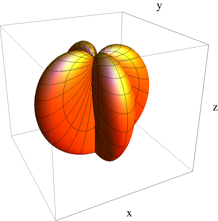
(a)

(b)

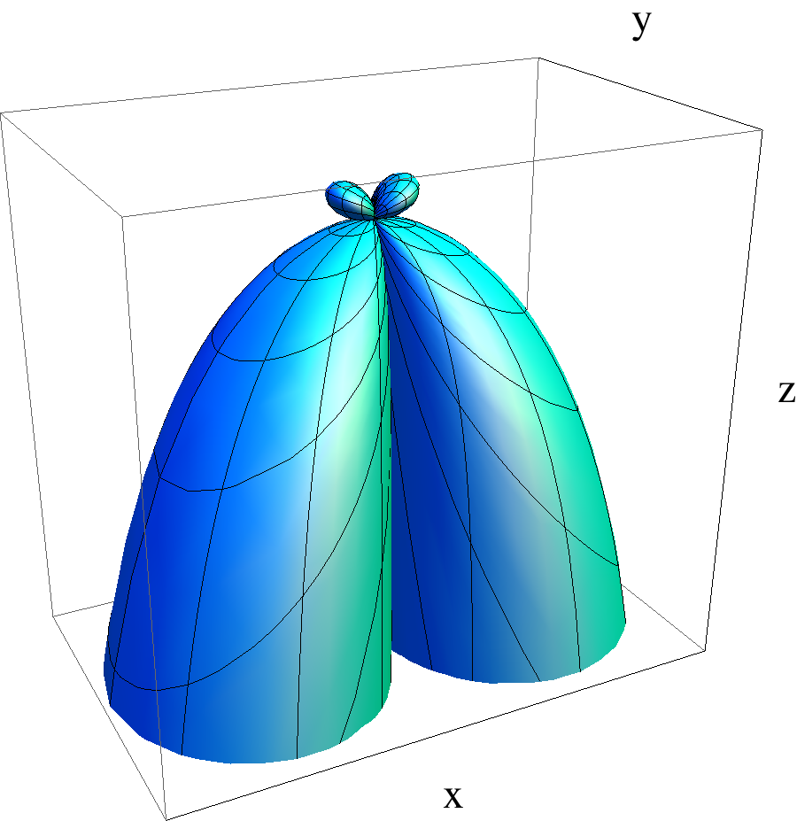
(c)

(d)

Figure 3: Antenna patterns (5) for plus/cross (a), breathing (b), vector-x/vector-y (c), and longitudinal (d) polarization modes. Note that the cross and vector-y modes are identical to plus and vector-x, respectively, but rotated by 45 degrees and thus do not appear separately here. In this figure, the GW propagates in the positive z-direction with the Earth at the origin, and the antenna pattern depends on the pulsar’s direction, specified by polar angle $\theta_{p}$ and azimuthal angle $\phi_{p}$. Exact expressions corresponding to each figure may be found in Appendix A: (A) for the plus mode, (A) for the breathing mode, (81) for the vector-x mode, and (61) for the longitudinal mode. Note that fixing the GW propagation direction while allowing the pulsar position to change is analogous to fixing the pulsar position while allowing the direction of GW propagation to change (there is an inherent degeneracy in the GW polarization angle and the pulsar’s azimuthal angle $\phi_{p}$).

The actual quantity measured in pulsar timing experiments is the timing residual, which is defined as the difference between the actual and expected time of arrival (TOA) of a pulse:

$$R(t)=\rm{TOA_{\hskip 2.84526ptactual}}-\rm{TOA_{\hskip 2.84526ptexpected}}.$$ (7)

The expected TOA for a pulse is modeled and includes daily and yearly motion of the Earth, the position and proper motion of the pulsar, motion about a binary companion (if applicable), etc. The timing residual can be obtained by integrating the redshift in time Detweiler (1979).

In Fig. 3 we plot the antenna patterns for the various GW polarization modes in a system where the GW’s direction of propagation is fixed and the pulsar’s position is varied (see Appendix A, Eqns. (A), (A), (81) and (61) for details), as is usually done in the literature.

III GW detection statistic

In this section we introduce the optimal cross correlation statistic Allen and Romano (1999); Anholm et al. (2009) for stochastic background searches. The optimal cross-correlation statistic involves the calculation of the overlap reduction function, a geometrical factor that characterizes the loss of sensitivity due to detectors not being co-located or aligned. We will show how the overlap reduction function is computed for non-transverse modes. We follow the analysis (for General Relativity) of Allen and Romano Allen and Romano (1999).

The plane wave expansion for a GW perturbation propagating in the direction $\hat{\Omega}$ is given by Allen and Romano (1999)

$$h_{ij}(t,\vec{x}) = \sum_{A}\int_{-\infty}^{\infty}df\int_{S^{2}}d\Omega e^{2\pi if(t-\hat{\Omega}\cdot\vec{x})}h_{A}(f,\hat{\Omega})\epsilon^{A}_{ij}(\hat{\Omega})$$

(8)

where $i,j$ are spatial indices, the sum is over all six polarization states, and the Fourier amplitudes $h_{A}(f,\hat{\Omega})$ are complex functions satisfying $h_{A}(-f,\hat{\Omega})=h_{A}^{*}({f,\hat{\Omega}})$. A stochastic background of GWs is produced by a large number of weak, independent, unresolvable sources. The energy density of this background per unit logarithmic frequency is given by

$$\Omega_{\rm{gw}}(f)=\frac{1}{\rho_{\rm{critical}}}\frac{d\rho_{\rm{gw}}}{d\ln{f}}$$ (9)

where $d\rho_{\rm{gw}}$ is the energy density of the gravitational waves and $\rho_{\rm{critical}}$ is the critical energy density required to close the universe,

$$\rho_{\rm{critical}}=\frac{3H_{0}^{2}}{8\pi G}$$ (10)

where $H_{0}$ is the Hubble constant.

The characteristic strain spectrum, $h_{c}(f)$, is typically given a power-law dependence on frequency so that

$$h_{c}(f) = A\left(\frac{f}{\rm{yr}^{-1}}\right)^{\alpha}.$$ (11)

It may also be expressed in terms of the energy density of the background per unit logarithmic frequency, $\Omega_{\rm{gw}}(|f|)$:

$$h^{2}_{c}(f) = \frac{3H_{0}^{2}}{2\pi^{2}}\frac{1}{f^{2}}\Omega_{\rm{gw}}(|f|).$$ (12)

For an isotropic stochastic background of GWs, the signal appears in the data as correlated noise between measurements from different pulsars. The $i^{th}$ data set is of the form

$$s_{i}(t) = z_{i}(t)+n_{i}(t)$$ (13)

where $z_{i}(t)$ corresponds to the unknown GW signal and $n_{i}(t)$ to noise (assumed in this case to be stationary and Gaussian). Because the signal is assumed to be much smaller than the noise, the properties of the noise determine the variance. We can express these properties in the frequency domain as

$$\langle\tilde{n}_{i}(f)\rangle = 0$$ (14)

$$\langle\tilde{n}^{*}_{i}(f)\tilde{n_{j}}(f^{\prime})\rangle = \frac{1}{2}\delta(f-f^{\prime})P_{i}(|f|)$$ (15)

where we have introduced the one-sided noise power spectrum $P_{i}(|f|)$.

The cross-correlation statistic is defined as

$$S=\int_{-T/2}^{T/2}dt\int_{-T/2}^{T/2}dt^{\prime}s_{i}(t)s_{j}(t^{\prime})Q(t-t^{\prime})$$ (16)

where $Q(t-t^{\prime})$ is the filter function. The optimal filter is determined by maximizing the expected signal-to-noise ratio

$$\rm{SNR}=\frac{\mu}{\sigma}.$$ (17)

Here $\mu$ is the mean $\langle S\rangle$ and $\sigma$ is the square root of the variance $\sqrt{\langle S^{2}\rangle-\langle S\rangle^{2}}$.

In the frequency domain (16) becomes

$$S=\int_{-\infty}^{\infty}df\int_{-\infty}^{\infty}df^{\prime}\delta_{T}(f-f^{\prime})\tilde{s}^{*}_{i}(f)\tilde{s}_{j}(f^{\prime})\tilde{Q}(f^{\prime}),$$ (18)

and the mean $\mu$ is

$$\mu = \int_{-\infty}^{\infty}df\int_{-\infty}^{\infty}df^{\prime}\,\delta_{T}(f-f^{\prime})\langle\tilde{z}_{i}^{*}(f)\tilde{z}_{j}(f^{\prime})\rangle\tilde{Q}(f^{\prime})$$

where $\delta_{T}$ is the finite time approximation to the delta function

$$\delta_{T}(f)=\frac{\sin{\pi ft}}{\pi f}.$$

The assumption that the background is unpolarized, isotropic, and stationary implies that the expectation value of the Fourier amplitudes $h_{A}(f,\hat{\Omega})$ must satisfy Allen and Romano (1999); Anholm et al. (2009)

$$\langle h^{*}_{A}(f,\hat{\Omega})h_{A^{\prime}}(f^{\prime},\hat{\Omega}^{\prime})\rangle = \frac{3H_{0}^{2}}{32\pi^{3}}\delta^{2}(\hat{\Omega},\hat{\Omega}^{\prime})\delta_{AA^{\prime}}$$

$$\times \delta(f-f^{\prime})|f|^{-3}\Omega_{gw}(|f|)$$

where $\delta^{2}(\hat{\Omega},\hat{\Omega}^{\prime})$ is the covariant Dirac delta function on the two-sphere. With the demand (III) in place, the expectation value of the signals $z_{i}(f)$ may be written as

$$\langle\tilde{z}_{i}^{*}(f)\tilde{z}_{j}(f^{\prime})\rangle = \frac{3H_{0}^{2}}{32\pi^{3}}\frac{1}{\beta}\delta(f-f^{\prime})|f|^{-3}$$

$$\times \Omega_{\rm{gw}}(|f|)\Gamma(|f|).$$

Here $\beta$ is a normalization factor and we define Anholm et al. (2009)

$$\Gamma(|f|) = \beta\sum_{A}\int_{S^{2}}d\Omega\,(e^{2\pi ifL_{i}(1+\hat{\Omega}\cdot\hat{p}_{i})}-1)$$

$$\times (e^{-2\pi ifL_{j}(1+\hat{\Omega}\cdot\hat{p}_{j})}-1)F_{i}^{A}(\hat{\Omega})F_{j}^{A}(\hat{\Omega})$$

where the sum is over all possible GW polarizations, and the exponential phase terms correspond to the pulsar term in the time domain.

The optimal filter is given by Allen and Romano (1999); Anholm et al. (2009)

$$\tilde{Q}(f)\propto\frac{\Omega_{\rm{gw}}(f)\Gamma(f)}{|f|^{3}P_{i}(f)P_{j}(f)},$$ (23)

where $P_{i}(f)$ and $P_{j}(f)$ are the power spectra for the $i$th and $j$th pulsar redshift time series that are being cross-correlated (see Eq. 16).

In general relativity, for the frequency and distance ranges appropriate to pulsar timing experiments (i.e. for $f\gg 1/L$), the overlap reduction function $\Gamma(f)$ approaches a constant which is only a function of the angular separation between the two pulsars. This constant is proportional to the value of the Hellings-Downs curve for the angle between the pulsars Hellings and Downs (1983); Anholm et al. (2009). We will see that for longitudinal modes and for tensor modes the overlap reduction function remains frequency dependent, even for $f\gg 1/L$, and is considerably larger than for the transverse modes. This indicates an increased sensitivity to such modes. To understand the physical origin of the increased sensitivity we first discuss the effect of GWs in the more simple case of a single pulsar-Earth baseline.

IV GW induced redshift on the pulsar-Earth system

In this section we will study the redshifts induced by GWs of different polarizations on the pulsar-Earth system. From (6), the redshift induced by this GW may be written as

$$\tilde{z}_{A}(f,\hat{\Omega})=\left(e^{-2\pi ifL(1+\hat{\Omega}\cdot\hat{p})}-1\right)\frac{p^{i}p^{j}}{2(1+\hat{\Omega}\cdot\hat{p})}\epsilon_{ij}^{A}(\hat{\Omega})\tilde{h}_{A}.$$

The factor of $1/2(1+\hat{\Omega}\cdot\hat{p})$ comes from the relationship between the affine parameter $\lambda$ and time $t$ (see Eq. (58)), and $\tilde{h}_{A}=\tilde{h}_{A}(f,\hat{\Omega})$.

In the region where the GW direction, $\hat{\Omega}$ and the pulsar direction, $\hat{p}$ are anti-parallel, (IV) appears to become singular due to the $1+\hat{\Omega}\cdot\hat{p}$ term in the denominator (note that the derivative of $h_{A}$ with respect to the affine parameter vanishes in this limit; see  (58)). There is in fact no divergence in the redshift induced. In this regime the exponential can be Taylor expanded and the $1+\hat{\Omega}\cdot\hat{p}$ term in the denominator cancels.

A Taylor expansion of (IV) can be performed in two cases. In the first, when $fL\ll 1$, the metric perturbation is the same at the pulsar and at the Earth. This case is often referred to as the long wavelength limit. In the second, when

$$1+\hat{\Omega}\cdot\hat{p}\ll\frac{1}{fL},$$

the pulse’s direction of propagation and the GW are nearly parallel (i.e. the GW is coming from a direction near the pulsar). In this case the metric perturbation at the pulsar when the pulse is emitted, and on Earth when the pulse is received, are also nearly the same. This is often described in the literature in terms of the pulse “surfing” the gravitational wave.

The surfing description, combined with Eq. (1), might lead one to incorrectly conclude that the effect of the GW should cancel in this case because the metric perturbations at the Earth and the pulsar are the same, despite the divergent $1/(1+\hat{\Omega}\cdot\hat{p})$ term in the redshift. In fact, a delicate cancellation occurs with the divergent term in the denominator which is only manifest in the frequency domain. Let the pulse direction and the gravitational wave direction be nearly parallel so that $\hat{\Omega}\cdot\hat{p}=-1+\delta$, where $\delta\ll 1$. Then as in Anholm et al. (2009); Tinto and Alves (2010) we obtain

$$\tilde{z}_{A}(f,\hat{\Omega})\sim-\pi ifLp^{i}p^{j}\epsilon_{ij}^{A}\tilde{h}_{A}.$$ (25)

The redshift is proportional to $fL$, but for finite $\delta$ increases only to the point where the argument of the exponential in (IV) can no longer be Taylor expanded, at which point it becomes an oscillatory function of $fL$. Whether the redshift is finite in the $\delta\rightarrow 0$ limit depends on the projection term $p^{i}p^{j}\epsilon_{ij}^{A}h_{A}$. As we will see, the vanishing contribution for the tensor modes of general relativity occurs solely because of the transverse nature of these waves, and is unrelated to the “surfing” effect. For longitudinal modes the projection term does not vanish, and the increase in sensitivity to such modes originates from GWs that come from directions near the pulsar. To better understand this, we will look at the behavior of the redshifts induced by GWs of various modes.

The redshift for a longitudinal mode GW perturbation is

$$\tilde{z}_{l}(f,\hat{\Omega}) = \frac{\cos^{2}{\theta}}{2(1+\cos{\theta})}(e^{-2\pi ifL(1+\cos{\theta})}-1)\tilde{h}_{l},$$ (26)

while the redshift for a plus mode GW perturbation is

$$\tilde{z}_{+}(f,\hat{\Omega}) = \frac{-\sin^{2}{\theta}}{2(1+\cos{\theta})}(e^{-2\pi ifL(1+\cos{\theta})}-1)\tilde{h}_{+}.$$ (27)

Here we note that the geometrical factor in the redshift for the transverse breathing mode differs from (27) only by a sign, and our analysis of (27) applies equally to the breathing mode.

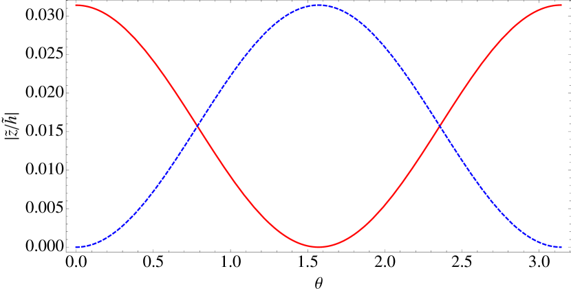
(a)

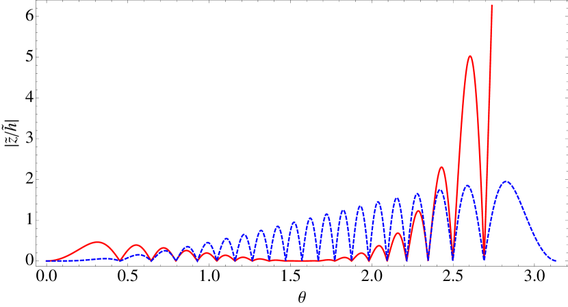
(b)

Figure 4: (color online) Plots of $|\tilde{z}(f,\hat{\Omega})/\tilde{h}|$ for the $+$-mode (dashed blue) and the longitudinal mode (solid red). We show these for $fL=10^{-2}$ (a), a value of $fL$ in the long wavelength limit, and (b) $fL=10$, a value of $fL$ typical of pulsar timing experiments. In the regime of pulsar timing experiments the sensitivity is largest for GW directions near the pulsar $\theta\approx\pi$ for both polarizations. In the longth wavelength limit, $fL\ll 1$, the pulsar-Earth system is most sensitive to $+$-mode GWs coming from the equator, and longitudinal GWs from the poles.

In Fig. 4 we plot the geometrical and phase factor $|\tilde{z}(f,\hat{\Omega})/\tilde{h}|$ for both the $+$-mode and the longitudinal mode. We plot these for a value of $fL$ in the long wavelength limit ($fL=10^{-2}$), and for a value in the regime of pulsar timing experiments ($fL=10$). In the regime of pulsar timing experiments the sensitivity is largest for GW directions near the pulsar $\theta\approx\pi$ for both polarizations. Although we do not show it here the same is true for all other polarization modes. In the long wavelength limit, $fL\ll 1$, the pulsar-Earth system is most sensitive to $+$-mode GWs coming from the equator, and longitudinal GWs from the poles.

As discussed above, these redshifts appear to become singular when $\theta\rightarrow\pi$, but the pulsar term may be Taylor expanded. Let $\theta=\pi-\delta$, where $\delta\ll 1$. Then

$$\tilde{z}_{l}(f,\hat{\Omega})\sim\pi ifL(1-\delta^{2})\tilde{h}_{l}$$ (28)

for the longitudinal case, while

$$\tilde{z}_{+}(f,\hat{\Omega})\sim\pi ifL\delta^{2}\tilde{h}_{+}$$ (29)

for the plus mode. In the limit as $\delta\rightarrow 0$, $\tilde{z}_{+}$ vanishes while $\tilde{z}_{l}$ becomes proportional to $fL$. The vanishing redshift of $\tilde{z}_{+}$ is therefore due to the transverse nature of the mode, and does not occur for $\tilde{z}_{l}$, even though in both cases the pulse is “surfing” the GW. In the time domain, in the $\theta\approx\pi$ region, the redshift for both modes goes as

$$z_{l,+}(t,\hat{\Omega})\propto L\dot{h}_{l,+}.$$ (30)

One may readily identify the right hand side of (30) as a velocity. The interpretation of this result is that, in this limit, the redshift is proportional to the relative velocity of the pulsar-Earth system. The velocity of the pulsar when the pulse is emitted in this limit is approximately equal and opposite to the velocity of the Earth when the pulse is received.

An identical analysis for the shear GW modes produces analogous results. Starting from (6), the redshift for the vector-y mode goes as

$$\tilde{z}_{y}(f,\hat{\Omega}) = -\frac{\cos{\theta}\sin{\theta}}{(1+\cos{\theta})}(e^{-2\pi ifL(1+\cos{\theta})}-1)h_{y}.$$ (31)

The small $\delta$ expansion yields

$$\tilde{z}_{y}(f,\hat{\Omega})\sim-2\pi ifL\delta\left(1-\frac{\delta^{2}}{2}\right)h_{y}.$$ (32)

Relative to the longitudinal mode the redshift of vector modes is smaller by a factor of $\delta$ and vanishes as $\delta\rightarrow 0$, but it is still larger than the transverse modes by a factor of $1/\delta$.

The same behavior is not present in other sky locations. If the GW propagates perpendicular to the pulsar-Earth line ($\theta~{}=~{}\pi/2~{}+~{}\delta$), then up to second order in $\delta$ the redshifts

$$\tilde{z}_{l} = \frac{\delta^{2}}{2(1-\delta)}\left(e^{-2\pi ifL(1-\delta)}-1\right)\mbox{ (longitudinal)}$$ (33)

$$\tilde{z}_{+} = \frac{-\left(1-\delta^{2}\right)}{2(1-\delta)}\left(e^{-2\pi ifL(1-\delta)}-1\right)\mbox{ (plus)}$$ (34)

$$\tilde{z}_{y} = \frac{\delta\left(1-\delta^{2}/2\right)}{(1-\delta)}\left(e^{-2\pi ifL(1-\delta)}-1\right)\mbox{ (shear)}$$ (35)

are obtained. In this case for small $\delta$ the exponential cannot be expanded unless $fL\ll 1$. For this sky location the redshift is always an oscillatory function of $fL$. The pulse comes across different phases of the GW as it propagates toward Earth.

To summarize, one can see that the surfing effect does not lead to a vanishing response of the pulsar-Earth system to GW waves coming from $\theta=\pi$. For the tensor and scalar-breathing modes, it is the transverse nature of GWs that is responsible for the vanishing response. For the scalar-longitudinal modes the response does not vanish—in fact, the response increases with both frequency and pulsar distance. For the vector modes the response does vanish, but more slowly than for the transverse modes. For all GW modes from directions near $\theta=\pi$, the redshift increases monotonically up to some limiting frequency beyond which the Taylor series expansion of the pulsar term which leads to Eqs. (28) and (29) can no longer be performed.

We now discuss the implications of this effect on the overlap reduction functions.

V Overlap reduction functions

As discussed in Section III, the overlap reduction function for the two pulsars in Fig. 1 is equal to

$$\Gamma(|f|) = \frac{3}{4\pi}\sum_{A}\int_{S^{2}}d\Omega(e^{2\pi ifL_{1}(1+\hat{\Omega}\cdot\hat{p}_{1})}-1)$$

$$\times (e^{-2\pi ifL_{2}(1+\hat{\Omega}\cdot\hat{p}_{2})}-1)F_{1}^{A}(\hat{\Omega})F_{2}^{A}(\hat{\Omega})$$

$$= \Gamma_{+}(|f|)+\Gamma_{\times}(|f|)+\Gamma_{b}(|f|)+\Gamma_{l}(|f|)$$

$$+ \Gamma_{x}(|f|)+\Gamma_{y}(|f|)$$

where all possible GW polarizations are allowed. It is advantageous to consider each term in the sum (V) separately since various gravity theories may have different polarization content Will (1993); Nishizawa et al. (2009); Lobo (2008); Alves et al. (2009); Capozziello and Francaviglia (2008); De Felice and Tsujikawa (2010); Brunetti et al. (1999); Clifton et al. (2011); Sagi (2010); Clifton et al. (2010); Skordis (2009); Milgrom (2009).

Figure 5: Hellings and Downs Hellings and Downs (1983) first showed that for general relativity, an isotropic stochastic background of GWs is expected to produce the correlation shown in blue. The correlation for the transverse breathing mode appears in black.

The overlap reduction function has a closed analytic form for transverse GWs. The overlap reduction function for the plus mode has been calculated by Hellings and Downs (1983) and is given by

$$\Gamma_{+}(\xi)=3\left[\frac{1}{3}+\frac{1-\cos{\xi}}{2}\left[\log{\left(\frac{1-\cos{\xi}}{2}\right)}-\frac{1}{6}\right]\right],$$ (38)

where $\xi$ is the angular separation of the pulsars. For the scalar-breathing mode, a closed form is given by Lee et al. (2008):

$$\Gamma_{b}(\xi)=\frac{1}{4}\left(3+\cos{\xi}\right).$$ (39)

For the case of non-transverse GWs, the overlap reduction functions cannot be integrated analytically and we calculate them numerically.

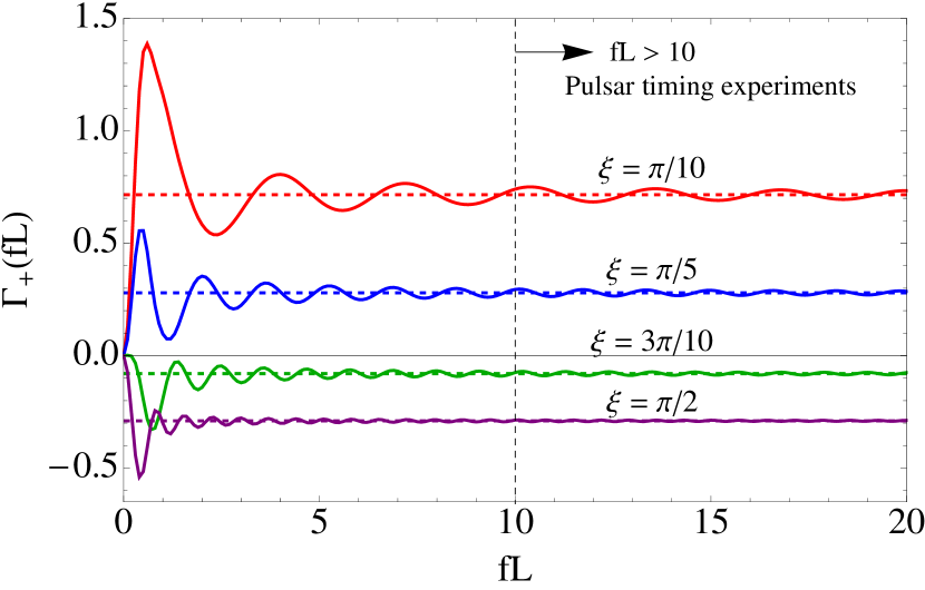
(a)

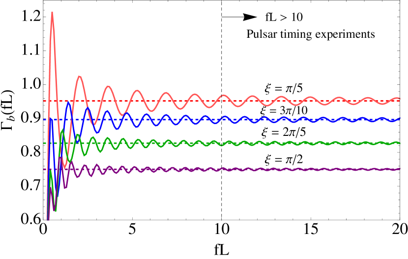
(b)

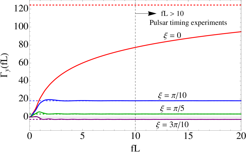
(c)

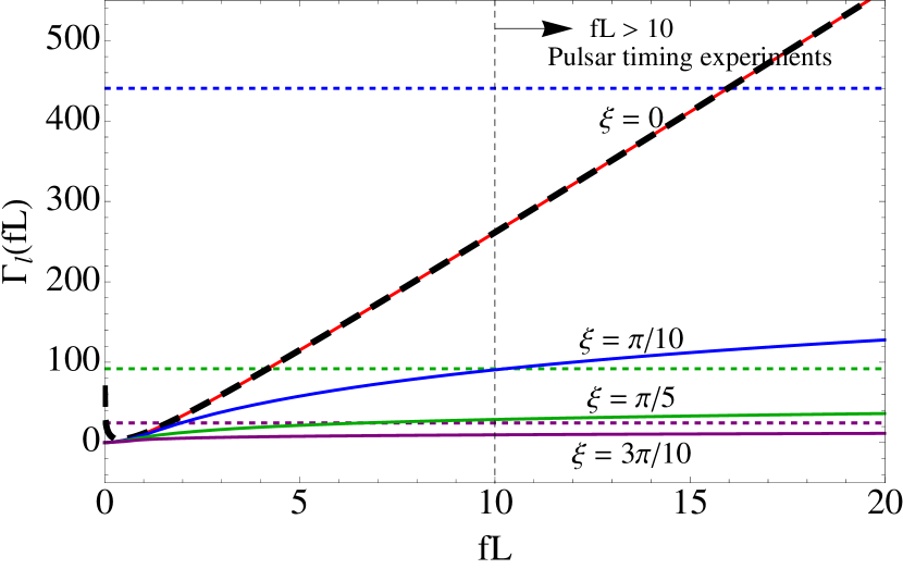
(d)

Figure 6: (color online) $\Gamma(fL)$ with (solid curves) and without (horizontal dashed lines) the pulsar term for the various polarization modes: plus (a), breathing (b), shear (c) and longitudinal (d). In the latter two modes, smaller pulsar separation angles are characterized by retained frequency dependence in $\Gamma(fL)$ in the range of frequencies relevant to pulsar timing experiments. Nearly all the non-transverse curves eventually converge, but at rather high values of $\Gamma(fL)$ relative to the transverse modes, indicating increased sensitivity to GWs with these polarizations. We have plotted the large limit approximation (41) (dashed black curve) along with $\Gamma_{l}(fL)$ in (d), which is in good agreement with the $\xi=0$ curve.

In general relativity the pulsar term can be excluded from the integral (V) without any significant loss of optimality Anholm et al. (2009). The reason for this is that the smallest frequencies that PTAs are sensitive to are $\sim 0.1$ yr^-1, and the closest PTA pulsar distances are $\sim 100$ ly, so that $fL\gtrsim 10$. This is shown in Fig. 6, where we plot the overlap reduction functions $\Gamma(fL)$ with (solid curves) and without (horizontal dashed lines) the pulsar term for several pulsar separation angles $\xi$ and GW polarization modes. The frequencies that PTAs are sensitive to are to the right of the vertical dashed line at $fL=10$ in each plot. As seen in Fig. 6(a), $\Gamma_{+}(fL)$ is roughly independent of frequency over the range of frequencies relevant to pulsar timing experiments. The same is true for the scalar-breathing mode, which is shown in Fig. 6(b). It is worth pointing out that both $\Gamma_{+}(fL)$ and $\Gamma_{b}(fL)$ are normalized to unity for co-aligned pulsars. Note that the overlap reduction functions for all other modes are normalized with the same factor of $3/4\pi$ used in the $+$-mode.

In Fig. 6(c), we plot the overlap reduction function $\Gamma_{y}(fL)$ for the vector-y mode. Over the range of relevant frequencies, $\Gamma_{y}(fL)$ is frequency independent for most of the pulsar separation angles shown. For co-aligned pulsars, however, $\Gamma_{y}(fL)$ retains frequency dependence well into the range of pulsar timing frequencies, and takes on values an order of magnitude higher than those obtained by $\Gamma_{+}(fL)$ and $\Gamma_{b}(fL)$.

Similar behavior is shown in Fig. 6(d), where we have plotted the overlap reduction function for the scalar-longitudinal mode. Here $\Gamma_{l}(fL)$ retains frequency dependence throughout the relevant frequency range for each of the pulsar separation angles shown. For the case of co-aligned pulsars, $\Gamma_{l}(fL)$ does not converge, and for separation angles that do converge $\Gamma_{l}(fL)$ takes on values that are at least an order of magnitude larger than those obtained by $\Gamma_{+}(fL)$ and $\Gamma_{b}(fL)$.

For co-located pulsars we can understand the behavior of the longitudinal mode analytically. In the problematic sky region ($\theta\approx\pi$), $\Gamma_{l}(fL)$ is proportional to the square of the redshift,

$$\Gamma_{l}(fL) \propto 2\pi\int_{-1}^{1}\left|\left(e^{-2\pi ifL(1+\cos{\theta})}-1\right)\right|^{2}$$ (40)

$$\times \frac{\cos^{4}{\theta}}{4(1+\cos{\theta})^{2}}\hskip 2.84526ptd{(\cos{\theta})}$$

which may be evaluated analytically. In the limit of large $fL$,

$$\Gamma_{l}(fL) = \pi\left\{37/6-4\gamma-1/(\pi(fL)^{2})+4\text{ Ci}({4\pi fL})\right.$$ (41)

$$- \left.4\log{(4\pi fL)}+2\pi fL\text{ Si}({4\pi fL})\right\}\text{ ($fL\gg 1$)}$$

$$\sim \left(37/6-4\gamma\right)\pi-4\pi\log{(4\pi fL)}+{\pi}^{3}fL,$$

where $\gamma$ is Euler’s constant. The overlap reduction function $\Gamma_{l}(fL)$ is roughly proportional to $fL$ in this limit. Eq. (41) is shown along with the numerically integrated overlap reduction functions in Fig. 6(d) and, with the exception of the singular behavior near the origin (where the large $fL$ approximation is not valid), agrees well with the numerical $\Gamma_{l}(fL)$ curve for co-aligned pulsars ($\xi~{}=~{}0$).

VI Overlap reduction functions for the NANOGrav pulsars

The NANOGrav PTA consists of 24 pulsars. The Australia Telescope National Facility (ATNF) data for the distances to these pulsars is given in Table 1 Manchester et al. (2005). Using a simple numerical integration scheme, the overlap reduction function for each pulsar pair was computed. The main difference relative to the previous section is that we are including the effect of different pulsar distances. Results are given in Fig. 7 (a)–(d) and show that the calculated values of $\Gamma(f)$ are consistent with the more simple results discussed in Section V for the non-transverse modes for frequencies up to $\sim 10^{-9}$ Hz.

PSR	Distance (kpc)			PSR	Distance (kpc)
J0030$+$0451	0.23			J1853$+$1303	1.60
J0218$+$4232	5.85			J1857$+$0943	0.70
J0613$-$0200	2.19			J1903$+$0327	6.45
J1012$+$5307	0.52			J1909$-$3744	0.55
J1024$-$0719	0.35			J1910$+$1256	1.95
J1455$-$3330	0.74			J1918$-$0642	1.40
J1600$-$3053	2.67			J1939$+$2134	3.58
J1640$+$2224	1.19			J1944$+$0907	1.28
J1643$-$1224	4.86			J1955$+$2908	5.39
J1713$+$0747	0.89			J2010$-$1323	1.29
J1738$+$0333	1.97			J2145$-$0750	0.50
J1744$-$1134	0.17			J2317$+$1439	1.89

Table 1: NANOGrav Pulsar Data

Pulsar pairs with the smallest ($\xi\lesssim 12^{\circ}$) separation angles (starred curves in Fig. 7 (b), (d)) for non-transverse polarization modes are characterized by large values of the overlap reduction function and monotonic growth up to some limiting frequency. Pulsar pairs with larger ($\xi\gtrsim 12^{\circ}$) separation angles (un-starred curves in Fig. 7 (b), (d) and all curves in Fig. 7) do not display monotonic growth up to a limiting frequency, but still result in much larger values than those of the plus and cross modes. Fig. 7 shows that sensitivity is greater for scalar-longitudinal and vector modes than for the tensor and scalar-breathing modes, and increases rapidly for pulsars that are nearly co-aligned in the sky.

Over the entire range of frequencies plotted for pulsar timing experiments (between $\sim 10^{-9}$ and $\sim 10^{-7}$ Hz), the overlap reduction functions are approximately constant. In practice, some optimality will be lost due to the fact that pulsar distances are known at best to only $\sim 10\%$ Cordes and Lazio (2002).

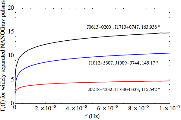
(a)

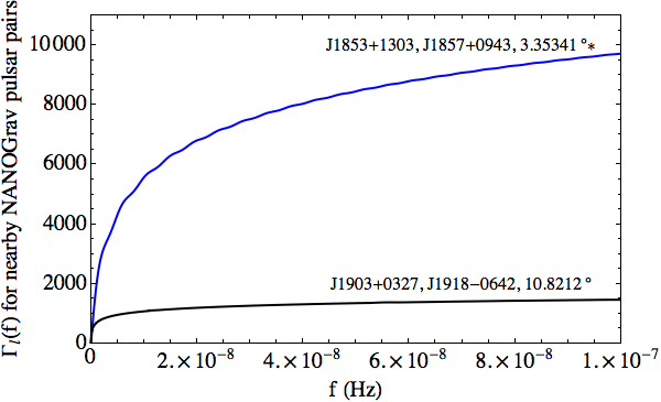
(b)

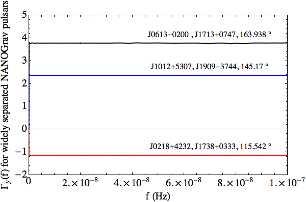
(c)

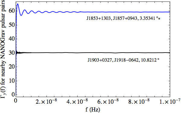
(d)

Figure 7: $\Gamma(f)$ for some of the NANOGrav pulsar pairs. Pulsar pairs, along with their angular separation in degrees, are shown with each curve. As $f$ increases, $\Gamma(f)$ approaches a constant value. The asterisk indicates the NANOGrav pulsar pair with the smallest angular separation ($\sim 3.35$ degrees). Note the larger values of the $\Gamma(f)$s for this pair.

VII Discussion

Direct detection of GWs might be possible in the next decade using a pulsar timing array. A detection would provide a mechanism for testing various metric theories of gravity. To develop optimal detection strategies for stochastic backgrounds in alternative theories of gravity, we have computed overlap reduction functions for all six GW polarization modes, including four modes not present in general relativity.

We began by introducing the redshift induced by GWs of various polarizations, along with the polarization tensors unique to each mode. We then used the optimal detection statistic for an unpolarized, isotropic stochastic background of GWs, defined in Anholm et al. Anholm et al. (2009), to find the overlap reduction function, a geometric dependent quantity in the expression for the expected cross correlation.

We examined the redshifts induced by GWs of various polarizations on the pulsar-Earth system, and find that our results are consistent with those of Anholm et al. Anholm et al. (2009) and Tinto and Alves Tinto and Alves (2010): when the GWs are coming from roughly the same direction as the pulses from the pulsar, the induced redshift for any GW polarization mode is proportional to $fL$, the product of the GW frequency and the distance to the pulsar. When the GWs and the pulse direction are exactly parallel the redshift for the transverse and vector modes vanishes, but it is proportional to $fL$ for the scalar-longitudinal mode.

We show that the vanishing contributions from the tensor, vector and scalar-breathing modes are not a result of the pulse surfing the GW. In fact, sensitivity to GWs coming from directions near the pulsar increases for all polarizations. It is the transverse nature of these modes that is responsible for the vanishing response. In this limit we also show that the redshift is proportional to the relative velocity of the pulsar-Earth system ($L\dot{h}$), which is the same when the pulse is emitted and when it is received.

We find that the overlap reduction functions for non-transverse GWs are characterized by frequency dependence that is significant for nearby pulsar pairs. The values of the overlap reduction function increase by up to one order of magnitude for the vector polarization modes and up to two orders of magnitude for the scalar-longitudinal mode. Pulsar timing arrays are significantly more sensitive to scalar-longitudinal and vector GW stochastic backgrounds.

Next, we used current pulsar distance and sky-location data from the ATNF pulsar catalog to calculate the overlap reduction functions for each pulsar pair in the NANOGrav pulsar timing array. Over the range of frequencies relevant to pulsar timing array experiments, these overlap reduction functions for all polarization modes are roughly constant for most pulsar pairs. For nearly co-aligned pulsars, the overlap reduction functions for scalar-longitudinal and vector modes exhibit marked frequency dependence and asymptote to much larger values than the overlap reduction functions for transverse modes. In fact for a pair separated but about $3^{\circ}$ we find a sensitivity increase of about a factor of $10^{4}$ for longitudinal modes.

The results discussed here may be compared to other recent work. Lee et al. Lee et al. (2008) calculated the cross-correlation functions for stochastic GW backgrounds including all six GW polarizations, and found that the correlation functions for non-transverse GWs are frequency dependent, as well as an increased response in the cross-correlation to scalar-longitudinal GWs, in agreement with our results. This work was done in the context of the coherence statistic Lee et al. (2008) for stochastic background detection, rather than the optimal statistic Anholm et al. (2009). The coherence statistic is a measure of goodness of fit of the pulsar-pair cross-correlations to the Hellings-Downs curve. For non-transverse modes there is no Hellings-Downs curve because the overlap reduction functions remain frequency dependent for large $fL$. Lee et al. solved this problem by simulating GW backgrounds and finding effective background-dependent Hellings-Downs curves for these theories. In the context of the optimal statistic this is a non-issue: The frequency dependent overlap reduction functions can be used to construct the optimal filter in Eq. (23). This is identical to what is done for LIGO stochastic background optimal filter construction Allen and Romano (1999), where the overlap reduction functions are also frequency dependent.

Alves and Tinto Alves and Tinto (2011) have estimated antenna sensitivities to GWs of all six polarization modes by assuming a signal-to-noise ratio of 1 over 10 years and calculating the noise spectrum. Their results indicate an increase of two to three orders of magnitude in sensitivity to scalar-longitudinal mode GWs compared to that of plus and cross mode GWs. To explain this effect Alves and Tinto compare the effect of a tensor GW propagating orthogonally to the pulsar-Earth system, and a scalar-longitudinal GW propagating in a direction parallel to the pulse direction. They argue that the increased sensitivity to longitudinal GWs is due to the amount of time a longitudinal GW affects the pulsar-Earth radio link.

We have compared the effect of GW propagation from directions near the pulsar and orthogonal to the pulsar-Earth system for all polarization modes. For GW propagation directions parallel to the pulse direction we find that the redshift induced by a gravitational wave is large, and seemingly divergent when the GW and pulse directions are exactly parallel. This apparent divergence occurs for longitudinal, transverse, and shear modes alike. In that limit, however, the divergent term in the redshift that comes from the relationship between time and affine parameter derivatives cancels because the phase of the GW pulse when pulse is emitted is nearly equal to the phase of the GW when the pulse is received (see Eqs. (58), (IV) and (25)). The redshift becomes proportional to the relative velocity of the pulsar-Earth system and a mode-dependent geometrical projection factor for all GW polarization modes. In this limit the relative velocity of the pulsar-Earth system is approximately equal when the pulse is emitted and received. For transverse and shear modes the projection factor vanishes when the GW and pulse directions become parallel. For longitudinal modes the geometrical factor goes to a constant, so that the pulsar-Earth system is very sensitive to GWs from directions near the pulsar. This is the physical origin of the increased sensitivity to scalar-longitudinal GWs.

Appendix A Analog to Detweiler’s equation for vector and scalar polarization modes

Here we show the derivation of the redshift induced by non-Einsteinian GW modes. This derivation appears in Tinto and Alves (2010) for all six GW polarizations and is included here for completeness. We begin by considering the metric due to a longitudinal mode gravitational wave perturbation:

$$g_{ab} = \eta_{ab}+h_{ab}(t-z)$$ (46)

$$= \left(\begin{array}[]{cccc}-1&0&0&0\\ 0&1&0&0\\ 0&0&1&0\\ 0&0&0&1+h_{L}\end{array}\right).$$

Given a null vector $s^{a}=\nu(1,-\alpha,-\beta,-\gamma)$ in Minkowski space (where $\alpha\text{, }\beta\text{, }\gamma$ are directional cosines) the corresponding perturbed null vector is given by

$$\sigma^{a} = s^{a}-\frac{1}{2}\eta^{ab}h_{bc}s^{c}$$ (51)

$$= \nu\left(\begin{array}[]{c}1\\ -\alpha\\ -\beta\\ -\gamma(1-\frac{h_{L}}{2})\end{array}\right).$$

From the geodesic equation, the t-component of $\sigma^{a}$ must satisfy

$$\frac{d\sigma^{t}}{d\lambda} = -\Gamma^{t}_{ab}\sigma^{a}\sigma^{b}$$ (52)

where

$$\Gamma^{t}_{ab} = \frac{1}{2}g^{tc}\left(\partial_{a}g_{bc}+\partial_{b}g_{ac}-\partial_{c}g_{ab}\right)$$ (53)

$$= \frac{1}{2}\dot{g}_{ab}.$$

Now we may write the geodesic equation as

$$\frac{d\sigma^{t}}{d\lambda} = -\frac{1}{2}\dot{g}_{ab}\sigma^{a}\sigma^{b}$$ (54)

$$= -\frac{1}{2}\dot{h_{L}}(\sigma^{z})^{2}.$$

To zeroth order in $h_{L}$,

$$(\sigma^{z})^{2} = \nu^{2}\gamma^{2}\left(1+\frac{h_{L}}{2}\right)^{2}$$ (55)

$$\approx \nu^{2}\gamma^{2}+O(h_{L})$$

allowing us to write the geodesic equation as

$$\frac{d\sigma^{t}}{d\lambda} = \frac{d\nu}{d\lambda}=-\frac{1}{2}\dot{h_{L}}\nu^{2}\gamma^{2}.$$ (56)

We now need to express the time derivative of the metric perturbation, $\dot{h_{L}}$, as a derivative of the affine parameter $\lambda$. Since $h_{L}=h_{L}(t-z)$, we may write

$$\frac{dh_{L}}{d\lambda} = \frac{\partial h_{L}}{\partial t}\frac{dt}{d\lambda}+\frac{\partial h_{L}}{\partial z}\frac{dz}{d\lambda}$$ (57)

$$= \frac{\partial h_{L}}{\partial t}\frac{dt}{d\lambda}-\frac{\partial h_{L}}{\partial t}\frac{dz}{d\lambda}.$$

Identifying the relations $\frac{dt}{d\lambda}=\nu$ and $\frac{dz}{d\lambda}=-\nu\gamma$, we obtain the relation

$$\dot{h_{L}}=\frac{\partial h_{L}}{\partial t}=\frac{1}{\nu(1+\gamma)}\frac{dh_{L}}{d\lambda}$$ (58)

which makes the geodesic equation

$$\frac{d\nu}{d\lambda} = -\frac{1}{2}\dot{h_{L}}\nu^{2}\gamma^{2}=-\frac{1}{2}\frac{\nu\gamma^{2}}{(1+\gamma)}\frac{dh_{L}}{d\lambda}$$ (59)

Integrating both sides, we obtain

$$\frac{\nu_{e}}{\nu_{p}}=\exp{\left(-\frac{1}{2}\frac{\gamma^{2}}{(1+\gamma)}\Delta h_{L}\right)}$$ (60)

where $\Delta h_{l}=h^{e}_{l}-h^{p}_{l}$. Expanding to first order in $h_{L}$, we may write

$$\frac{\nu_{e}-\nu_{p}}{\nu_{p}} \approx -\frac{1}{2}\frac{\gamma^{2}}{(1+\gamma)}\Delta h_{L}$$ (61)

$$= -\frac{\cos^{2}{\theta_{p}}}{2\left(1+\cos{\theta_{p}}\right)}\Delta h_{L}.$$ (62)

The derivation for vector modes is nearly identical to that of the longitudinal mode. For the sake of brevity we only detail the vector-y mode in the remainder of this document. For the vector-y mode, the metric perturbation takes the form

$$g_{ab}=\left(\begin{array}[]{cccc}-1&0&0&0\\ 0&1&0&0\\ 0&0&1&h_{y}\\ 0&0&h_{y}&1\end{array}\right).$$ (67)

The null vector becomes

$$\sigma^{a}=\nu\left(\begin{array}[]{c}1\\ -\alpha\\ -\beta+\frac{h_{y}\gamma}{2}\\ \frac{h_{y}\beta}{2}-\gamma\end{array}\right).$$ (72)

Following the same algebraic steps used above, one obtains the geodesic equation

$$\frac{d\sigma^{t}}{d\lambda} = \frac{d\nu}{d\lambda}=-\dot{h_{y}}\nu^{2}\gamma\beta,$$ (73)

which leads to

$$\frac{d\nu}{d\lambda}=-\frac{\nu\gamma\beta}{(1+\gamma)}\frac{dh_{y}}{d\lambda}.$$ (74)

Integrating this expression and expanding the result to first order in $\Delta h_{y}$ produces the result

$$\frac{\nu_{e}-\nu_{p}}{\nu_{p}} \approx -\frac{\beta\gamma}{(1+\gamma)}\Delta h_{y}$$ (75)

$$= -\frac{\sin{2\theta_{p}}\sin{\phi_{p}}}{2\left(1+\cos{\theta_{p}}\right)}\Delta h_{y}.$$ (76)

where $\Delta h_{y}=h^{e}_{y}-h^{p}_{y}$.

For comparison, we also include the results for the plus, cross, vector-x, and breathing modes. For the plus mode, we obtain

$$\frac{\nu_{e}-\nu_{p}}{\nu_{p}} \approx -\frac{\left(\alpha^{2}-\beta^{2}\right)}{2(1+\gamma)}\Delta h_{+}$$

$$= -\frac{\sin^{2}{\theta_{p}}\cos{2\phi_{p}}}{2\left(1+\cos{\theta_{p}}\right)}\Delta h_{+};$$

for the cross mode,

$$\frac{\nu_{e}-\nu_{p}}{\nu_{p}} \approx -\frac{\alpha\beta}{(1+\gamma)}\Delta h_{\times}$$ (79)

$$= -\frac{\sin^{2}{\theta_{p}}\sin{2\phi_{p}}}{2\left(1+\cos{\theta_{p}}\right)}\Delta h_{\times};$$ (80)

for the vector-x mode,

$$\frac{\nu_{e}-\nu_{p}}{\nu_{p}} \approx -\frac{\alpha\gamma}{(1+\gamma)}\Delta h_{x}$$ (81)

$$= -\frac{\sin{2\theta_{p}}\cos{\phi_{p}}}{2\left(1+\cos{\theta_{p}}\right)}\Delta h_{x};$$ (82)

and for the breathing mode,

$$\frac{\nu_{e}-\nu_{p}}{\nu_{p}} \approx -\frac{\left(\alpha^{2}+\beta^{2}\right)}{2(1+\gamma)}\Delta h_{b}$$

$$= \frac{-\sin^{2}{\theta_{p}}}{2\left(1+\cos{\theta_{p}}\right)}\Delta h_{b}.$$

Here, $\Delta h_{A}=h_{A}^{e}-h_{A}^{p}$, and we can identify these expressions with (2).

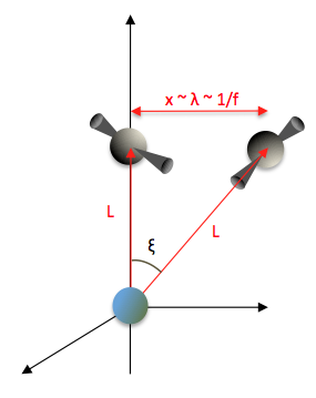
Figure 8: A system of two pulsars, distance $L$ form the Earth, are shown along with their separation angle $\xi$ and separation distance $x\approx L\xi$. When the GW is in the long wavelength limit, this separation distance is proportional to the GW wavelength.

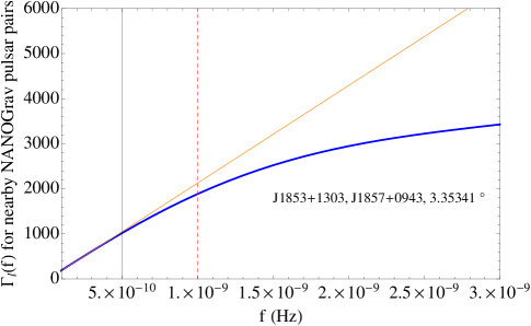
Figure 9: The NANOGrav pulsar pair $J1853+1303$, $J1857+0943$ has an angular separation of nearly $3^{\circ}$, with each pulsar approximately $1$ kpc from the Earth. Using the estimate (86), the curve $\Gamma_{l}(f)$ should stop growing as $\sim\pi^{3}fL$ near $10^{-9}$ Hz, which is shown as the red vertical dashed line. Note, however, that the curve does not converge onto constant values of $\Gamma_{l}(f)$ at this point; in fact the overlap reduction function continues to grow well past this point, but no longer linearly with $fL$ (as indicated by orange solid line).

 

Appendix B Trends in $\Gamma_{l}(f)$ for nearby pulsar pairs

Consider a pair of pulsars separated by some small angle $\xi$ and located approximately equidistant from the Earth so that $L_{1}\sim L_{2}\equiv L$.

As shown in Section V, if the two pulsars are co-located the overlap reduction function $\Gamma_{l}(f)\sim\pi^{3}fL$. We expect that if they are separated by a small angle the overlap reduction function will increase as $\pi^{3}fL$ as though they were co-located, until the wavelength of the GW is comparable to the distance between the two pulsars. This happens when

$$\lambda\sim L\xi,$$ (85)

so that the value of $fL$ where the behavior changes from the co-located case is

$$fL\sim 1/\xi.$$ (86)

For example, for the closest NANOGrav pulsar pair, separated by an angle $\xi\sim 3^{\circ}$ at a distance of $L\sim 1$ kpc, the frequency at which the linear growth of the overlap reduction function stops is

$$f\sim 10^{-9}\text{ Hz}.$$ (87)

The value of of the overlap reduction function where the behavior changes from the co-located case $\Gamma_{l}(\xi^{-1})$ is a poor estimate of the maximum value of $\Gamma_{l}(f)$, however, because after exiting the linear regime of Eq. (41), the overlap reduction functions continue to increase significantly before converging.

A closer look at the lower frequency portion of the plot Fig. 7(b), shown in Fig. 9, indicates that to order of magnitude this approximation is roughly valid.

References

- Nojiri and Odintsov (2006) S. Nojiri and S. D. Odintsov, ArXiv High Energy Physics - Theory e-prints (2006), eprint arXiv:hep-th/0601213.
- Nojiri and Odintsov (2011) S. Nojiri and S. D. Odintsov, Phys. Rep. 505, 59 (2011), eprint 1011.0544.
- Lobo (2008) F. S. N. Lobo, ArXiv e-prints (2008), eprint 0807.1640.
- Alves et al. (2009) M. E. S. Alves, O. D. Miranda, and J. C. N. de Araujo, Phys. Lett. B 679, 401 (2009), eprint 0908.0861.
- Capozziello and Francaviglia (2008) S. Capozziello and M. Francaviglia, Gen. Rel. Grav. 40, 357 (2008), eprint 0706.1146.
- De Felice and Tsujikawa (2010) A. De Felice and S. Tsujikawa, Living Rev. Rel. 13 (2010), eprint 1002.4928.
- Will (1993) C. M. Will, Theory and Experiment in Gravitational Physics (Cambridge University Press, 1993).
- Brunetti et al. (1999) M. Brunetti, E. Coccia, V. Fafone, and F. Fucito, Phys. Rev. D 59, 044027 (1999), URL http://www.citebase.org/abstract?id=oai:arXiv.org:gr-qc/9805056.
- Clifton et al. (2011) T. Clifton, P. G. Ferreira, A. Padilla, and C. Skordis, ArXiv e-prints (2011), eprint 1106.2476.
- Sagi (2010) E. Sagi, Phys. Rev. D 81, 064031 (2010), eprint 1001.1555.
- Clifton et al. (2010) T. Clifton, M. Banados, and C. Skordis, Class. Quant. Grav. 27, 235020 (2010), eprint 1006.5619.
- Skordis (2009) C. Skordis, Class. Quant. Grav. 26, 143001 (2009), eprint 0903.3602.
- Milgrom (2009) M. Milgrom, Phys. Rev. D 80, 123536 (2009), eprint 0912.0790.
- Abramovici et al. (1992) A. Abramovici, W. E. Althouse, R. W. Drever, Y. Gursel, S. Kawamura, et al., Science 256, 325 (1992).
- Hobbs et al. (2010) G. Hobbs, A. Archibald, Z. Arzoumanian, D. Backer, M. Bailes, et al., Class. Quant. Grav. 27, 084013 (2010), eprint 0911.5206.
- Sesana et al. (2008) A. Sesana, A. Vecchio, and C. N. Colacino, Mon. Not. R. Astron. Soc. 390, 192 (2008), eprint 0804.4476.
- Olmez et al. (2010) S. Olmez, V. Mandic, and X. Siemens, Phys. Rev. D 81, 104028 (2010), eprint 1004.0890.
- Starobinsky (1979) A. A. Starobinsky, JETP Lett. 30, 682 (1979).
- Caprini et al. (2010) C. Caprini, R. Durrer, and X. Siemens, Phys. Rev. D 82, 063511 (2010), eprint 1007.1218.
- Nishizawa et al. (2009) A. Nishizawa, A. Taruya, K. Hayama, S. Kawamura, and M.-a. Sakagami, Phys. Rev. D 79, 082002 (2009), URL http://link.aps.org/doi/10.1103/PhysRevD.79.082002.
- Lee et al. (2008) K. J. Lee, F. A. Jenet, and R. H. Price, Astrophys. J. 685, 1304 (2008), URL http://stacks.iop.org/0004-637X/685/i=2/a=1304.
- Alves and Tinto (2011) M. E. d. S. Alves and M. Tinto, Phys. Rev. D 83, 123529 (2011), URL http://link.aps.org/doi/10.1103/PhysRevD.83.123529.
- Detweiler (1979) S. Detweiler, Astrophys. J. 234, 1100 (1979).
- Anholm et al. (2009) M. Anholm, S. Ballmer, J. D. E. Creighton, L. R. Price, and X. Siemens, Phys. Rev. D 79, 084030 (2009), URL http://link.aps.org/doi/10.1103/PhysRevD.79.084030.
- Allen and Romano (1999) B. Allen and J. D. Romano, Phys. Rev. D 59, 102001 (1999), URL http://link.aps.org/doi/10.1103/PhysRevD.59.102001.
- Eardley et al. (1973) D. M. Eardley, D. L. Lee, A. P. Lightman, R. V. Wagoner, and C. M. Will, Phys. Rev. Lett. 30, 884 (1973), URL http://link.aps.org/doi/10.1103/PhysRevLett.30.884.
- Tinto and Alves (2010) M. Tinto and M. E. d. S. Alves, Phys. Rev. D 82, 122003 (2010), URL http://link.aps.org/doi/10.1103/PhysRevD.82.122003.
- Hellings and Downs (1983) R. W. Hellings and G. S. Downs, Astrophys. J. 265, L39 (1983).
- Manchester et al. (2005) R. N. Manchester, G. B. Hobbs, A. Teoh, and M. Hobbs, Astrophys. J. 129, 1993 (2005), URL http://stacks.iop.org/1538-3881/129/i=4/a=1993.
- Cordes and Lazio (2002) J. M. Cordes and T. J. W. Lazio, ArXiv Astrophysics e-prints (2002), eprint arXiv:astro-ph/0207156.