Lie algebra solution of population models based on time-inhomogeneous Markov chains

Abstract

Many natural populations are well modelled through time-inhomogeneous stochastic processes. Such processes have been analysed in the physical sciences using a method based on Lie algebras, but this methodology is not widely used for models with ecological, medical and social applications. This paper presents the Lie algebraic method, and applies it to three biologically well motivated examples. The result of this is a solution form that is often highly computationally advantageous.

1 Introduction

Stochastic models based on Markov chains are important in many ecological, medical and social contexts. In these contexts, where populations are modelled, there are often external influences that act on the system in a manner that varies over time, leading to a time-inhomogeneous Markov chain model and corresponding technical difficulties for analysis [10].

Wei and Norman [14] proposed a method for dealing analytically with time-inhomogeneous Markov chains, based on Lie algebraic methods. The idea of combining Lie algebras and symmetry considerations with Markov chains has continued to attract theoretical interest in a variety of contexts [15, 6, 9, 12].

At the same time, there is a more applied desire to have numerically efficient methods to analyse Markov-chain population models, one option for which is the use of matrix exponentials [8, 10]. The aim of this paper is to explain how Lie algebraic methods can be used to derive matrix exponential solutions to time-inhomogeneous Markov chains that are applicable to population modelling. In contrast to other applications, symmetries of these systems are not a guide to the appropriate Lie algebra to use in solution of population models; a certain amount of trial and error is necessary. The focus of this paper is therefore on three examples in population modelling where it is possible to define an appropriate Lie algebra, and a discussion of the potential benefits of doing so.

2 Methodology

2.1 Lie algebras

In general, a Lie algebra over a field $F$ is an $F$-vector space $V$, together with a bilinear map called the Lie bracket. Elements of the vector space are written $u,v,w\in V$. The Lie bracket is written $[u,v]\in V$ and obeys

$$[u,u]=0\text{ ,}\qquad[u,[v,w]]+[v,[w,u]]+[w,[u,v]]=0\text{ .}$$ (1)

We will be interested in the vector space $GL(n,{\mathbb{R}})$, i.e. the set of real-valued $n\times n$ matrices, and will define the Lie bracket for $X,Y\in GL(n,{\mathbb{R}})$ through the commutator

$$[X,Y]:=XY-YX\text{ ,}$$ (2)

which can be readily seen to satisfy (1). It is often convenient to define an adjoint endomorphism operator, ad, to represent the Lie bracket:

$$(\text{ad}X)Y:=[X,Y]\text{ ,}$$ (3)

so that multiple applications of the Lie bracket can be concisely written as e.g. $(\text{ad}X)^{2}Y=[X,[X,Y]]$ .

2.2 Time-inhomogeneous Markov processes

Suppose that $p(t)$ is a probability vector, i.e. a vector with values $p_{n}(t)\geq 0$ summing to unity that represent the probability that an integer stochastic variable takes the value $n$ at time $t$. We consider models in which the evolution of these probabilities over time is given by

$$\frac{dp}{dt}=H(t)p(t)\text{ ,}$$ (4)

where $H(t)$ is a time-dependent matrix such that at any time $t$ its off-diagonal elements are positive and its column sums are zero. This defines a time-inhomogeneous continuous-time Markov chain. For some special cases, analytic solutions can be obtained. But in general, where the state-space of the Markov chain is finite, numerical algorithms exist that calculate $p(t)$ by making use of expansions such as

$$p(t+\delta t)=H(t)p(t)\delta t+O(\delta t^{2})\text{ ,}$$ (5)

and accumulating a sufficient number of $\delta t$ steps to reach $p(t)$ from $p(0)$. Methods based on this direct integration will therefore calculate $p(t)$ in $O(t)$ operations.

2.3 The method of Wei and Norman

In this section, we recall the methodology of Wei and Norman [14], which is applicable to equations of the form (4) above. The first step is to look for a decomposition of $H(t)$

$$H(t)=\sum_{i=1}^{m}a_{i}(t)H_{i}\text{ ,}$$ (6)

where the $H_{i}$ are linearly independent matrices obeying

$$[H_{i},H_{j}]=H_{i}H_{j}-H_{j}H_{i}=\sum_{k}{\xi_{ij}}^{k}H_{k}\text{ ,}$$ (7)

for (in our case real-valued) scalars ${\xi_{ij}}^{k}$. Given such matrices, we can form a vector space $V=\text{span}\{H_{i}\}_{i=1}^{m}\subseteq GL(n,{\mathbb{R}})$ such that for a Lie bracket as defined in (2), we have $[X,Y]\in V$ for all $X,Y\in V$. This closure under the action of the Lie bracket can be used to look for solutions of the form

$$p(t)=e^{g_{1}(t)H_{1}}\cdots e^{g_{m}(t)H_{m}}p(0)=:U(t)p(0)\text{ ,}$$ (8)

where matrix exponentiation is defined through the power series in the standard way. Using the ad operator as defined in (3), the Baker-Campbell-Hausdorff formula is

$$e^{X}Ye^{-X}=e^{(\text{ad}X)}Y\text{ ,}$$ (9)

which will enable us to derive the solution form advertised. Substituting (6) and (8) into (4) then gives

$$\frac{dp}{dt} =\sum_{i=1}^{m}a_{i}(t)H_{i}U(t)p(0)$$ (10)

$$=\sum_{i=1}^{m}\dot{g}_{i}(t)\left(\prod_{j=1}^{i-1}e^{g_{j}(t)H_{j}}\right)H_{i}\left(\prod_{j=i}^{m}e^{g_{j}(t)H_{j}}\right)p(0)\text{ .}$$

Since this expression holds for any $p(0)$, we can equate the operators acting on $p(0)$, postmultiply by $U^{-1}$, and repeatedly apply (9) to obtain

$$\sum_{i=1}^{m}a_{i}(t)H_{i}=\sum_{i=1}^{m}\dot{g}_{i}(t)\left(\prod_{j=1}^{i-1}e^{g_{j}(t)(\text{ad}{H_{j}})}\right)H_{i}\text{ .}$$ (11)

The precise solution to this equation will depend on the constants $\xi$ in (7), however since the $H_{i}$ are chosen to be linearly independent, terms in (11) in front of the same basis matrix can be equated, leading to a set of ODEs for the $g_{i}(t)$.

The usefulness of this method therefore depends on whether appropriate $H_{i}$ matrices can be defined, so that the equations that must be solved for $g_{i}(t)$ are not excessively complex. But in the event that $g_{i}(t)$ can be calculated in $O(1)$ rather than, say, $O(t)$ – which will typically be the case if an analytic result is obtained – then the computation of $p(t)$ can be achieved in $O(1)$ rather than $O(t)$ through the numerical calculation of the matrix exponentials in (8). Such enhanced computational tractability of stochastic models clearly has benefits in the application of probability theory to statistical inference, where the speed of evaluation of likelihoods is highly important.

3 Examples

The primary difficulty in applying the method above to population models is finding an appropriate expansion of the form (6), since the systems involved are not obviously symmetric. We now turn to three examples where an appropriate expansion can be found. In two cases, special initial conditions give analytic results that can be checked against other methods to confirm the soundness of the approach; and in the third, a significant numerical benefit is observed compared to direct integration.

3.1 A birth-death process

Suppose we have a time-inhomogeneous birth-death process, characterised by a stochastic variable $N(t)\geq 0$ taking integer values $n$, and the transition rates

$$n \rightarrow n+1\text{ at rate }b(t)\text{ ,}$$ (12)

$$n \rightarrow n-1\text{ at rate }nd(t)\text{ .}$$

A biological interpretation of this process would be the survival of juvenile animals, introduced to an inhospitable region by seasonal breeding happening at another site, and dying at a rate that depends on the climate. Defining components of a vector $p_{n}(t)=\Pr(N(t)=n)$, the Kolmogorov equation for this process is

$$\frac{dp}{dt}=(b(t)(R-\mathbb{1}{})+d(t)(L-M))p\text{ .}$$ (13)

The matrices involved are countably infinite in dimension, and are defined implicitly by (12) and (13). It is also possible to write explicit definitions in terms of the Kronecker delta:

$$(\mathbb{1}{})_{n,k}=\delta_{n,k}\text{ ; }\ (R)_{n,k}=\delta_{n,k+1}\text{ ; }\ (L)_{n,k}=(k-1)\delta_{n,k-1}\text{ ; }\ (M)_{n,k}=k\delta_{n,k}\text{ .}$$ (14)

Clearly, the identity matrix commutes with everything (i.e. $[\mathbb{1}{},X]=0$ for any $X$) while the other matrices obey

$$[L,R]=\mathbb{1}{}\text{ ,}\quad[M,R]=R\text{ ,}\quad[L,M]=L\text{ .}$$ (15)

We then look for solutions of the form

$$p(t)=e^{g_{1}(t)\mathbb{1}{}}e^{g_{2}(t)R}e^{g_{3}(t)L}e^{g_{4}(t)M}p(0)\text{ ,}$$ (16)

noting that $e^{g_{1}(t)\mathbb{1}{}}=e^{g_{1}(t)}$. Making use of the result (11) together with the algebra (15) gives

$$g_{1}(t) =-e^{\mathcal{D}(t)}\int_{0}^{t}b(u)e^{\mathcal{D}(u)}du\text{ ,}$$ (17)

$$g_{2}(t) =e^{\mathcal{D}(t)}\int_{0}^{t}b(u)e^{\mathcal{D}(u)}du\text{ ,}$$

$$g_{3}(t) =e^{\mathcal{D}(t)}-1\text{ ,}$$

$$g_{4}(t) =-\mathcal{D}(t)\text{ ,}$$

$$\text{where}\quad\mathcal{D}(t) :=\int_{0}^{t}d(u)du\text{ .}$$

This provides a solution to the original model, but one that is much simpler if we assume the initial condition $N(0)=0$, in which case

$$p_{n}(t)=e^{g_{1}(t)}\frac{\left(g_{2}(t)\right)^{n}}{n!}\text{ ,}$$ (18)

for $g_{1}$, $g_{2}$ as in (17). In this way an infinite-dimensional time-inhomogeneous Markov chain is reduced to carrying out the two integrals in (17). It is worth comparing this to the ‘textbook’ method for dealing with time-inhomogeneous Markov chains, which is to derive an expression for the probability generating function (PGF) [4]. This is done by writing down the Kolmogorov equation (13) in component form and substituting in the definition of the PGF, $G(s,t):=\sum_{n}s^{n}p_{n}(t)$. This gives a PDE for the PGF of

$$\frac{\partial G}{\partial t}=(b(t)s-d(t))(s-1)\frac{\partial G}{\partial s}\text{ ,}$$ (19)

which, given the initial condition $N(0)=0$, gives

$$G(s,t)=\text{exp}\left[(s-1)e^{-\mathcal{D}(t)}\int_{0}^{t}b(u)e^{\mathcal{D}(u)}du\right]\text{ .}$$ (20)

The equation (20) yields the same solution as (18) above through the standard relation

$$p_{n}=\frac{1}{n!}\left.\frac{\partial^{n}G}{\partial s^{n}}\right|_{s=0}$$ (21)

The effort in deriving the solution (18) through the PGF and Lie algebraic methods is therefore roughly similar; however the intermediate results obtained in each method are likely to be useful in different contexts. For example, the PGF in (20) is likely to be the easiest way to derive moments of the process; while the matrix exponential form (16) is likely to be useful if the derivative of the solution with respect to a parameter of the model is required [15].

3.2 Epidemic surveillance

Consider the following situation. An epidemic is in progress in a population, such that individuals are either susceptible to infection, infectious, or recovered and immune. Surveillance of the epidemic is carried out by recruitment of individuals at random from the general population (or more realistically through recruitment of individuals in contact with the healthcare system due to non-infectious illness) who are tested and determined to be either susceptible, infectious or recovered. The epidemic is characterised by a force of infection $\lambda(t)$, which is the rate at which susceptible individuals become infectious and for which there are various parametric forms [7], and also by a recovery rate $\gamma(t)$, which is the rate at which infectious individuals recover. A plausible explicit choice for these functions is to hold $\gamma(t)$ constant, and to take $\lambda(t)=\lambda_{0}e^{rt}$, representing the early exponential growth phase that is common to many different epidemics.

As other authors have found, manipulation of more complex Markov chains is simplified by the use of Dirac notation [6, 5, 2, 13]. In this formalism, the probability vector for the model described above is written

$$\left|p(t)\right>=\sum_{S,I}\Pr(S,I|N,t)\left|S,I\right>\text{ ,}$$ (22)

where $\Pr(S,I|N,t)$ is the probability that from a cohort of size $N$ a time $t$ after the start of the epidemic a number $S$ of the cohort is susceptible and a number $I$ is infectious (leaving $N-S-I$ recovered individuals). $\left|S,I\right>$ is a basis vector, linearly independent of any other basis vector with different susceptible and infectious counts. Operators, marked out using a hat $\hat{\mathcal{O}}$, act on basis vectors to give linear combinations of basis vectors. For this system, we need the following operators:

$$\hat{S}\left|S,I\right> =S\left|S,I\right>\text{ ,}$$ (23)

$$\hat{I}\left|S,I\right> =I\left|S,I\right>\text{ ,}$$

$$\hat{\Delta}\left|S,I\right> =S\left|S-1,I\right>\text{ ,}$$

$$\hat{\rho}\left|S,I\right> =I\left|S,I-1\right>\text{ ,}$$

$$\hat{\tau}\left|S,I\right> =S\left|S-1,I+1\right>\text{ .}$$

The action of these operators can be described computationally as follows: $\hat{S}$ returns the number of susceptibles; $\hat{I}$ returns the number of infectives; $\hat{\Delta}$ returns the number of susceptibles and depletes these by one; $\hat{\rho}$ returns the number of infectives and depletes these by one; and $\hat{\tau}$ returns the number of susceptibles, depletes the susceptible population by one, and increases the infectious population by one. The dynamical model is then

$$\frac{d}{dt}\left|p(t)\right>=\left(\gamma{}(t)\left(\hat{\rho}-\hat{I}\right)+\lambda{}(t)\left(\hat{\tau}-\hat{S}\right)\right)\left|p(t)\right>\text{ .}$$ (24)

Note that while (24) does not make use of the operator $\hat{\Delta}$, it is necessary to include this to have an algebra that is closed under the action of the Lie bracket. The full set of Lie brackets is shown in Table 1, and the action of the exponential adjoint endomorphism is shown in Table 2. We then look for a solution of the form

$$\left|p(t)\right>=e^{g_{1}(t)\hat{\Delta}}e^{g_{2}(t)\hat{\tau}}e^{g_{3}(t)\hat{S}}e^{g_{4}(t)\hat{\rho}}e^{g_{5}(t)\hat{I}}\left|p(0)\right>\text{ .}$$ (25)

Going through the same procedure as before gives solution

$$g_{1}(t) =e^{\Lambda(t)}\left(1-e^{-\Lambda(t)}-\int_{0}^{t}\lambda(u)e^{-\Lambda(u)}e^{\Gamma(u)-\Gamma(t)}du\right)\text{ ,}$$ (26)

$$g_{2}(t) =e^{\Lambda(t)}\int_{0}^{t}\lambda(u)e^{-\Lambda(u)}e^{\Gamma(u)-\Gamma(t)}du\text{ ,}$$

$$g_{3}(t) =-\Lambda(t)\text{ ,}\quad g_{4}(t)=1-e^{-\Gamma(t)}\text{ ,}\quad g_{5}(t)=-\Gamma(t)\text{ ,}$$

$$\text{for}\quad\Lambda(t) :=\int_{0}^{t}\lambda(u)du\text{ ,}\quad\text{and}\quad\Gamma(t):=\int_{0}^{t}\gamma(u)du\text{ .}$$

To check this result, assuming $\left|p(0)\right>=\left|N,0\right>$ and substituting (26) into (25) gives

$$\Pr(S,I|N,t)=\left(\begin{array}[]{c}N!\\ S!I!(N-S-I)!\end{array}\right)(\pi_{1})^{S}(\pi_{2})^{I}(1-\pi_{1}-\pi_{2})^{N-S-I}\text{ ,}$$ (27)

where

$$\pi_{1}=e^{-\Lambda(t)}\text{ ,}\qquad\pi_{2}=\int_{0}^{t}\lambda(u)e^{-\Lambda(u)}e^{\Gamma(u)-\Gamma(t)}du\text{ .}$$ (28)

This is the form we would expect for this solution; considering each individual’s probability of remaining susceptible to be $\pi_{1}$ and being infections to be $\pi_{2}$, these should obey

$$\frac{d}{dt}\left(\begin{array}[]{c}\pi_{1}\\ \pi_{2}\end{array}\right)=\left(\begin{array}[]{cc}-\lambda(t)&0\\ \lambda(t)&-\gamma(t)\end{array}\right)\left(\begin{array}[]{c}\pi_{1}\\ \pi_{2}\end{array}\right)\text{ ,}$$ (29)

which has solution (28), and the independence of each individual leads to the multinomial distribution (27) for the cohort as a whole. As for the birth-death process, the analytic result obtained through Lie algebraic methods can be obtained otherwise, and which method is preferable will depend on which further calculations one wishes to undertake.

3.3 A pure birth process

Now suppose we have a pure birth process, characterised by a stochastic variable $N(t)$ and transition rate

$$n\rightarrow n+1\text{ at rate }a(t)+nb(t)\text{ .}$$ (30)

Special forms of $a(t)$, $b(t)$ have been used to model the formation of social contacts [1]. Defining components of a vector $p_{n}=\Pr(N(t)=n)$, and assuming that there is a maximum count of interest $m$, such that we only keep track of $\Pr(N(t)>m)$ as the final component of $p$, we write the Kolmogorov equation for this process as

$$\frac{dp}{dt}=(a(t)P_{1}+b(t)Q)p\text{ .}$$ (31)

The generating matrices $P_{1}$ and $Q$ are implicitly defined by (30), however an additional set of matrices are required to produce a vector space that is closed under the Lie bracket. These matrices take a similar form to $P_{1}$ and are indexed by integer $i$. The definition of the matrices used, in terms of the Kronecker delta, is

$$(Q)_{n,k}=k(\delta_{n,k+1}-\delta_{n,k})\text{ ,}\qquad(P_{i})_{n,k}=\delta_{n,k+i}-\delta_{n,k+i-1}\text{ .}$$ (32)

These matrices satisfy the commutation relations

$$[P_{i},P_{j}]=0\text{ ,}\qquad[P_{i},Q]=-iP_{i+1}+(i-1)P_{i}\text{ .}$$ (33)

Note that it is here that the assumption of a finite state space (i.e. the introduction of a maximum count of interest above) allows the solution method to work, since otherwise a countably infinite number of matrices would be needed. We then look for a solution of the form

$$p(t)=e^{f_{1}(t)P_{1}}\cdots e^{f_{m}(t)P_{m}}e^{g(t)Q}p(0)\text{ ,}$$ (34)

and make use of (11) to give the following system of equations:

$$\dot{f}_{1}(t)=a(t)\text{ ,}\quad\dot{g}(t)=b(t)\text{ ,}\quad\dot{f}_{i>1}(t)=(i-1)\dot{g}(t)\left[f_{i-1}(t)-f_{i}(t)\right]\text{ .}$$ (35)

These equations have solution

$${f}_{1}(t) =\mathcal{A}(t)=\int_{0}^{t}a(u)du\text{ ,}$$ (36)

$${g}(t) =\mathcal{B}(t)=\int_{0}^{t}b(u)du\text{ ,}$$

$${f}_{i>1}(t) =e^{-(i-1)\mathcal{B}(t)}\int_{0}^{t}a(u)\left(e^{\mathcal{B}(t)}-e^{\mathcal{B}(u)}\right)^{i-1}du\text{ .}$$

Figure 1 shows numerical results for this system for the simple choice

$$a(t)=1\text{ ,}\quad b(t)=\frac{1}{1+t}\text{ ,}\quad m=100\text{ ,}\quad N(0)=0\text{ .}$$ (37)

Note that for this initial condition, and due to the relations (33), we can write the solution as

$$p_{n}(t)=\left(e^{\sum_{i}f_{i}(t)P_{i}}\right)_{n,0}\text{ ,}$$ (38)

the evaluation of which which can be seen in Figure 1 to give a significant computational advantage, as implemented in EXPOKIT [11], compared to direct integration of (31) through Runge-Kutta, as implemented in the MATLAB function ode45, at large times. Perhaps unexpectedly, this is seen despite the relatively large value of $m$. These plots show that, while the ODE solver uses a more sophisticated relationship than (5) to obtain better than $O(t)$ performance, it is still much more sensitive to model time $t$ than the matrix exponential method.

There will, of course, be more complex systems where numerical integration via Runge-Kutta is impractical, but analytic integration is simple (e.g. if either $a(t)$ or $b(t)$ is a square wave rapidly oscillating between 0 and 1); for these systems the matrix exponential method will further outperform Runge-Kutta. But there will also be systems where direct numerical integration is straightforward and there is no simply obtained form for $f_{i}(t)$ and $g(t)$, meaning that the matrix exponential solution is not useful.

4 Discussion

This paper has considered the solution of time-inhomogeneous Markov chains in population modelling through the use of matrix exponentials. This is done using the method of Lie algebras originally developed for applications in physical sciences [14]. In contrast to physical applications, population models are often insufficiently symmetric to write down a well studied Lie algebra. In even the relatively simple pure birth process considered, a large number of basis matrices were needed to derive a matrix exponential solution; but despite this the exponential solution is useful if a derivative with respect to a model parameter is required [15], and perhaps more importantly often has a significant numerical advantage over direct integration of the ODE system [8]. Given the popularity of computationally intensive inference in modern population models [3], any such improvement in numerical efficiency of likelihood evaluation can have important practical benefits.

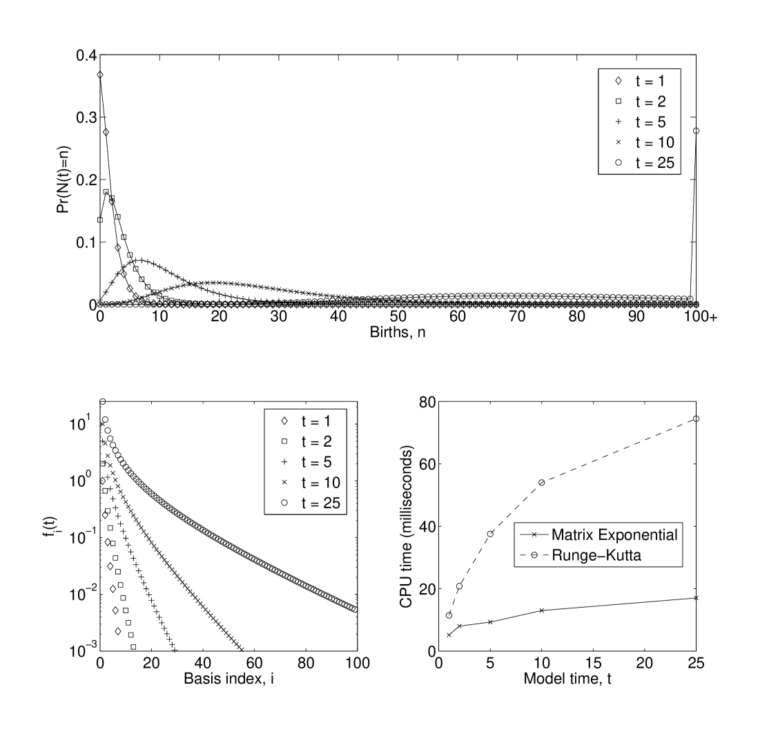
Figure 1: Numerical results for a time-inhomogeneous pure birth process. Top: probability distributions at different times. Matrix exponential solutions are shown with markers and direct integration via Runge-Kutta is shown with continuous black lines—clearly, these are numerically indistinguishable. Bottom left: values of the quantities $f_{i}$ over time. Bottom right: CPU time needed to run each method as a function of model time.

$\hat{X}$	$[\hat{X},\hat{S}]$	$[\hat{X},\hat{I}]$	$[\hat{X},\hat{\Delta}]$	$[\hat{X},\hat{\rho}]$	$[\hat{X},\hat{\tau}]$
$\hat{S}$	0	0	$-\hat{\Delta}$	0	$-\hat{\tau}$
$\hat{I}$	0	0	0	$-\hat{\rho}$	$\hat{\tau}$
$\hat{\Delta}$	$\hat{\Delta}$	0	0	0	0
$\hat{\rho}$	0	$\hat{\rho}$	0	0	$\hat{\Delta}$
$\hat{\tau}$	$\hat{\tau}$	$-\hat{\tau}$	0	$-\hat{\Delta}$	0

Table 1: Values of $[\hat{X},\hat{Y}]$ for the epidemic model.

$\hat{X}$	$e^{x(\text{ad}\hat{X})}\hat{S}$	$e^{x(\text{ad}\hat{X})}\hat{I}$	$e^{x(\text{ad}\hat{X})}\hat{\Delta}$	$e^{x(\text{ad}\hat{X})}\hat{\rho}$	$e^{x(\text{ad}\hat{X})}\hat{\tau}$
$\hat{S}$	$\hat{S}$	$\hat{I}$	$e^{-x}\hat{\Delta}$	$\hat{\rho}$	$e^{-x}\hat{\tau}$
$\hat{I}$	$\hat{S}$	$\hat{I}$	$\hat{\Delta}$	$e^{-x}\hat{\rho}$	$e^{x}\hat{\tau}$
$\hat{\Delta}$	$\hat{S}+x\hat{\Delta}$	$\hat{I}$	$\hat{\Delta}$	$\hat{\rho}$	$\hat{\tau}$
$\hat{\rho}$	$\hat{S}$	$\hat{I}+x\hat{\rho}$	$\hat{\Delta}$	$\hat{\rho}$	$\hat{\tau}+x\hat{\Delta}$
$\hat{\tau}$	$\hat{S}+x\hat{\tau}$	$\hat{I}-x\hat{\tau}$	$\hat{\Delta}$	$\hat{\rho}-x\hat{\Delta}$	$\hat{\tau}$

Table 2: Values of $e^{x(\text{ad}\hat{X})}\hat{Y}$ for the epidemic model, for scalar $x$.

References

- [1] Danon, L., House, T., Keeling, M. J. and Read, J. M. (2011). Collective properties of social encounter networks. To appear.
- [2] Dodd, P. J. and Ferguson, N. M. (2009). A many-body field theory approach to stochastic models in population biology. PLoS ONE 4, e6855.
- [3] Gilks, W. R., Richardson, S. and Spiegelhalter, D. J. (1995). Markov Chain Monte Carlo in Practice. Chapman and Hall/CRC.
- [4] Grimmett, G. R. and Stirzaker, D. R. (2001). Probability and Random Processes 3 ed. Oxford University Press.
- [5] Jarvis, P. D., Bashford, J. D. and Sumner, J. G. (2005). Path integral formulation and Feynman rules for phylogenetic branching models. Journal of Physics A: Mathematical and General 38, 9621.
- [6] Johnson, J. E. (1985). Markov-type Lie groups in . Journal of Mathematical Physics 26, 252–257.
- [7] Keeling, M. J. and Rohani, P. (2007). Modeling Infectious Diseases in Humans and Animals. Princeton University Press.
- [8] Keeling, M. J. and Ross, J. V. (2008). On methods for studying stochastic disease dynamics. Journal of The Royal Society Interface 5, 171–181.
- [9] Mourad, B. (2004). On a Lie-theoretic approach to generalised doubly stochastic matrices and applications. Linear and Multilinear Algebra 52, 99–113.
- [10] Ross, J. V. (2010). Computationally exact methods for stochastic periodic dynamics spatiotemporal dispersal and temporally forced transmission. Journal of Theoretical Biology 262, 14–22.
- [11] Sidje, R. B. (1998). Expokit. A software package for computing matrix exponentials. ACM Transactions on Mathematical Software 24, 130–156.
- [12] Sumner, J., Fernandez-Sanchez, J. and Jarvis, P. (2011). Lie Markov models. arXiv:1105.4680v1.
- [13] Sumner, J., Holland, B. and Jarvis, P. (2011). The algebra of the general Markov model on phylogenetic trees and networks. Bulletin of Mathematical Biology. Published online ahead of print. DOI:10.1007/s11538-011-9691-z.
- [14] Wei, J. and Norman, E. (1963). Lie algebraic solution of linear differential equations. Journal of Mathematical Physics 4, 575–581.
- [15] Wilcox, R. M. (1967). Exponential operators and parameter differentiation in quantum physics. Journal of Mathematical Physics 8, 962–982.