Decoherence suppression of open quantum systems through a strong coupling to non-Markovian reservoirs

Abstract

In this paper, we provide a mechanism of decoherence suppression for open quantum systems in general, and that for ”Schrodinger cat-like” state in particular, through the strong couplings to non-Markovian reservoirs. Different from the usual strategies of suppressing decoherence by decoupling the system from the environment in the literatures, here the decoherence suppression employs the strong back-reaction from non-Markovian reservoirs. The mechanism relies on the existence of the singularities (bound states) of the nonequilibrium retarded Green function which completely determines the dissipation and decoherence dynamics of open systems. As an application, we examine the decoherence dynamics of a photonic crystal nanocavity that is coupled to a waveguide. The strong non-Markovian suppression of decoherence for the optical cat state is attained.

I Introduction

How to protect quantum states away from decoherence is one of the most challenge topics in quantum information processing and modern quantum technology. During the past two decades, many schemes have been theoretically proposed and experimentally realized to suppress the decoherence in quantum information processing Feedback ; DFS ; DynDecoupling ; Yao07077602 ; UDD07100504 ; Du091265 . On the other hand, due to the significant development of the nanotechnology during the past decade, various quantum devices with high tunabilities, such as nanomechanical oscillator or superconducting qubit strongly coupled to cavity CirQED ; CavityMec , trapped atom coupled to an engineered reservoir AtomEngRes , arrays of coupled nanocavities in photonic crystal CavityCROW etc., can be engineered. In these quantum devices, the strong coupling between the system and the structured reservoir and the resulting non-Markovian back-action play an important role in the manipulations of quantum coherence.

In this work, we shall provide a general mechanism of decoherence suppression for quantum systems coupled strongly to non-Markovian reservoirs. Contrary to the ordinary means of suppressing decoherence via dynamically decoupling of the system from the environment DynDecoupling ; Yao07077602 ; UDD07100504 ; Du091265 , we employ the strong non-Markovian back-reaction from the environment to suppress the decoherence of quantum states. We show in general that when the non-Markovian back-reaction is strong enough, the decoherence of quantum states can be largely suppressed. In particular, we examine the time evolution of the Wigner function for a mesoscopic superposition of two coherent states, and demonstrate that the decoherence of such a mesoscopic superposition state can be suppressed due to the strong non-Markovian back-reaction from the environment.

II Exact Master Equation

The dynamics of open quantum systems are described by the reduced density matrix which can be obtained by tracing over all of the reservoir degrees of freedom form the total system $\rho(t)=\text{tr}[\rho_{\text{tot}}(t)]$, where $\rho_{\text{tot}}(t)$ is the total density matrix of the system plus its reservoir. The exact master equation of the reduced density matrix $\rho(t)$ for an open system, such as a cavity in quantum optics, a defect (nanocavity) in photonic crystals or a quantum dot in nanostructures, etc., coupled to a general non-Markovian reservoir has been derived recently Xio10012105 ; Wu1018407 ; Tu08235311 ; Lei

$$\frac{d\rho(t)}{dt}= \frac{1}{i}[H^{\prime}(t),\rho(t)]+\gamma(t)[2a\rho(t)a^{{\dagger}}-\rho(t)a^{{\dagger}}a-a^{{\dagger}}a\rho(t)]$$

$$+\tilde{\gamma}(t)[a\rho(t)a^{{\dagger}}+a^{{\dagger}}\rho(t)a-a^{{\dagger}}a\rho(t)-\rho(t)aa^{{\dagger}}]\ ,$$ (1)

where $H^{\prime}(t)=\omega^{\prime}(t)a^{{\dagger}}a$ is the renormalized Hamiltonian of the system with the renormalized frequency $\omega^{\prime}(t)=-\text{Im}[\dot{u}(t)u^{-1}(t)]$. The time-dependent coefficients $\gamma(t)=-\text{Re}[\dot{u}(t)u^{-1}(t)]$ and $\tilde{\gamma}(t)=\dot{v}(t)-2v(t)\text{Re}[\dot{u}(t)u^{-1}(t)]$ incorporates all of the dissipations and fluctuations induced from the coupling to the reservoir. The function $u(t)$ is the nonequilibrium retarded Green function of the system satisfying the following equation:

$$\dot{u}(t)+i\omega_{c}u(t)+\int_{t_{0}}^{t}g(t-\tau)u(\tau)=0$$ (2)

subjected to the initial condition $u(t_{0})=1$, and the nonequilibrium thermal fluctuation is characterized by the function $v(t)$ which is given by

$$v(t)=\int_{t_{0}}^{t}d\tau\int_{t_{0}}^{t}d\tau^{\prime}u^{*}(\tau_{1})\tilde{g}(\tau_{1}-\tau_{2})u(\tau_{2}).$$ (3)

By introducing the spectral density of the reservoir $J(\omega)=2\pi\sum_{k}|V_{k}|^{2}\delta(\omega-\omega_{k})$ where $V_{k}$ is the coupling between the system and the reservoir, the time correlation functions $g(\tau-\tau^{\prime})$ and $\tilde{g}(\tau-\tau^{\prime})$ in Eqs. (2-3) are given by

$$g(\tau-\tau^{\prime})=\int_{0}^{\infty}\frac{d\omega}{2\pi}J(\omega)e^{-i\omega(\tau-\tau^{\prime})}\ ,$$ (4)

$$\tilde{g}(\tau-\tau^{\prime})=\int_{0}^{\infty}\frac{d\omega}{2\pi}J(\omega)\bar{n}(\omega,T)e^{-i\omega(\tau-\tau^{\prime})}\ ,$$ (5)

which characterize all the non-Markovian back-reactions of the reservoir, and $\bar{n}(\omega,T)=\frac{1}{e^{\hbar\omega/k_{B}T}-1}$ is the average particle number distribution in the reservoir at the initial time $t_{0}$.

The decoherence dynamics of quantum states can be studied by examining the evolution of the corresponding Wigner function. With the help of the exact master equation (II), the exact Wigner function of an arbitrary quantum state at arbitrary time $t$ in the complex space $\{z\}$ is found:

$$W(z,t)=\int d\mu(\alpha_{0})d\mu(\alpha^{\prime}_{0})\langle\alpha_{0}|\rho(t_{0})|\alpha^{\prime}_{0}\rangle\mathfrak{J}(z,t|\alpha_{0},\alpha^{\prime*}_{0},t_{0}),$$ (6)

where $|\alpha\rangle=e^{\alpha a^{{\dagger}}}|0\rangle$ is the coherent state, $d\mu(\alpha)=\frac{d\alpha^{*}d\alpha}{2\pi i}e^{-|\alpha|^{2}}$ is the integral measure of the Bergmann complex space, $\rho(t_{0})$ is the reduced density matrix of the initial state, and the propagating function $\mathfrak{J}(z,t|\alpha_{0},\alpha^{\prime*}_{0},t_{0})$ is given by

$$\mathfrak{J}(z,t\ | \alpha_{0},\alpha^{\prime*}_{0},t_{0})=W_{0}(z,t)\exp\big{\{}z^{*}\Omega(t)u(t)\alpha_{0}$$

$$+\alpha^{\prime*}_{0}u^{*}(t)\Omega(t)z+\alpha^{\prime*}_{0}\big{(}1-|u(t)|^{2}\Omega(t)\big{)}\alpha_{0}\big{\}}\ ,$$ (7)

where $\Omega(t)=\frac{2}{1+v(t)}$ and $W_{0}(z,t)=\frac{\Omega(t)}{\pi}\exp{[\Omega(t)|z|^{2}]}$.

To concentrate on quantum decoherence, we examine the time evolution of a mesoscopic superposition of two coherent states moving in opposite directions, called as the ”Schrodinger cat-like” state or the optical cat state in the literature SCS : $|\phi\rangle=N(|\alpha\rangle+|-\alpha\rangle)$, where $N=1/\sqrt{4\cosh{|\alpha|^{2}}}$ is the normalization factor. As a result of Eq. (6), the time-evolution of the Wigner function for this cat state is given by

$$W(z,t)=W_{\alpha}(z,t)+W_{-\alpha}(z,t)+W_{I}(z,t)$$ (8a)

with

$$W_{\pm\alpha}(z,t)=N^{2}\frac{\Omega(t)}{\pi}e^{|\alpha|^{2}}e^{\Omega(t)|z\mp u(t)\alpha|^{2}}\ ,$$ (8b)

$$W_{I}(z,t) =2N^{2}\frac{\Omega(t)}{\pi}e^{-|\alpha|^{2}}\Re\big{\{}e^{-[z-u(t)\alpha]^{*}\Omega(t)[z+u(t)\alpha]}\big{\}}\ .$$ (8c)

In Eq. (8), the first two terms are the Wigner functions for the initial coherent states $|\alpha\rangle$ and $|-\alpha\rangle$ respectively, the third term is the interference between them. The quantum coherence of the cat state can then be characterized by the fringe visibility function

$$F(\alpha,t) \equiv\frac{1}{2}\frac{W_{I}(z,t)|_{\text{peak}}}{\sqrt{W_{\alpha}(z,t)|_{\text{peak}}W_{-\alpha}(z,t)|_{\text{peak}}}}$$

$$=\exp{\Big{\{}-2|\alpha|^{2}(1-\frac{|u(t)|^{2}}{1+2v(t)})\Big{\}}}$$ (9)

which ranges from unity to $\exp{(-2|\alpha|^{2})}$ for full coherence to complete decoherence. As shown by Eqs. (3), (8) and (II), the nonequilibrium retarded Green function $u(t)$ completely determine the dynamics of the quantum decoherence of the system. Equation (2) alone can also give the exact solution of atomic systems involving only single excitation (single photon process) at zero temperature Gar972290 ; Bre02 .

III General mechanism of decoherence suppression

The solution of the retarded Green function can be obtained by the inverse Laplace transformation Cohen ; Kofman ; Longhi $u(t)=\frac{1}{2\pi i}\int_{B}ds\tilde{u}(s)e^{st}$, where $\tilde{u}(s)=\frac{i}{is-\omega_{c}-\Sigma(s)}$ and the Bromwich path B is a line $\text{Re}(s)=\text{const}>0$ in the half plane of the analyticity of the transformation. The self-energy $\Sigma(s)=\int\frac{d\omega}{2\pi}\frac{J(\omega)}{is-\omega}$ is the Laplace transformation of the correlation function (4). Consider a spectral density ranged from $\omega_{e}$ to infinity, e.g. $\omega_{e}=0$ for Ohmic, super-Ohmic and sub-Ohmic reservoirs, etc. The self-energy is then not defined on the segment of the imaginary axis $s=-i\omega$ with $\omega>\omega_{e}$, while $s=-i\omega_{e}$ is a branch point. Near the imaginary axis, the self-energy function can be separated into real and imaginary parts by the relation $\lim_{\eta\rightarrow 0}\frac{1}{\omega\pm i\eta}={\cal P}\frac{1}{\omega}\mp i\pi\delta(\omega)$ so that $\Sigma(s=-i\omega\pm 0^{+})=\Delta(\omega)\mp i\frac{J(\omega)}{2}$ with $\Delta(\omega)={\cal P}\int^{\infty}_{\omega_{e}}\frac{d\omega^{\prime}}{2\pi}\frac{J(\omega^{\prime})}{\omega-\omega^{\prime}}$, and $\rm{\cal P}$ denotes the principal value. The analytic properties of the transformed retarded Green function $\tilde{u}(s)$ determine completely the decoherence dynamics of the system.

In the very weak coupling regime, the self-energy function is dominated near the pole $s=-i\omega_{c}$. The functions $\Delta(\omega)$ and $J(\omega)$ can be approximated by $\Delta_{c}=\Delta(\omega_{c})$ and $J_{c}=J(\omega_{c})$. The resulting retarded Green function becomes $u(t)=e^{-i\omega^{\prime}_{c}-\frac{J_{c}}{2}t}$ with the shifted frequency $\omega^{\prime}_{c}=\omega_{c}+\Delta_{c}$. The retarded Green function experiences an exponential decay with the decay constant $J_{c}/2$, which reproduces the Born-Markov result Xio10012105 ; Lei . Thus, $u(t)$ will eventually be damped to zero and the fringe visibility will be decayed to $\exp{(-2|\alpha|^{2})}$, namely the quantum coherence is totally lost.

However, as the coupling increases, the variation of the self-energy away from the pole $-i\omega_{c}$ becomes significant, and the decoherence dynamics of the system is then totally different from the Born-Makov limit. Especially, there exists an isolated pole $s=-i\Omega$ on the imaginary axis outside the branch cut, i.e. $\Omega-\omega_{c}=\Delta(\Omega)$ with $\Omega<\omega_{e}$, which leads to a dissipationless dynamics of the system.

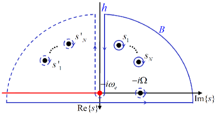
Figure 1: Integration contour of the inverse laplace transform of $\tilde{u}(s)$. The Red line on the imaginary axis is the branch cut. $-i\Omega$ is the pure imaginary pole. The integration along the solid (dashed) curve is made on the first (second) Riemannian sheet. $s_{i}$ and $s^{\prime}_{i}$ are the poles of $\tilde{u}(s)$ on the first and second Riemannian sheet in the $\text{Re}(s)<0$ half-plane.

The exact solution of the retarded Green function can be obtained by the inverse Laplace transform along the Bromwich path B as shown in Fig. 1. Since the closure crosses the branch cut $\text{Im}(s)<-\omega_{e}$ on the imaginary axis, the contour is necessary to pass into the second Riemannian sheet in the section of the half plane with $\text{Im}(s)<-\omega_{e}$, where it remains in the first Riemannian sheet in the sections $\text{Im}(s)>-\omega_{e}$ in the half plane $\text{Re}(s)<0$. To properly close the contour, it is necessary to turn around the branch point $-i\omega_{e}$, following the Hankel paths $h$ to enter and leave the second Riemannian sheet, as shown in Fig. 1. The exact propagating function can be obtained by means of the residue method

$$u(t)= \mathcal{Z}e^{-i\Omega t}+\sum_{i}\mathcal{Z}_{i}e^{-\gamma_{i}t-i\omega_{i}t}+\sum_{i}\mathcal{Z}^{\prime}_{i}e^{-\gamma^{\prime}_{i}t-i\omega^{\prime}_{i}t}$$

$$+\frac{1}{2\pi i}\int_{-\infty-i\omega_{e}}^{0-i\omega_{e}}ds\big{[}\tilde{u}^{\text{II}}(s)-\tilde{u}^{\text{I}}(s)\big{]}e^{st}\ ,$$ (10)

where $\mathcal{Z}$ is the residues of the bound state with the imaginary pole $s=-i\Omega$, $\mathcal{Z}_{i}$($\mathcal{Z}^{\prime}_{i}$) is the residues of the $i$th unstable states with the pole $s=s_{i}=-\gamma_{i}-i\omega_{i}$ ($s^{\prime}_{i}=-\gamma^{\prime}_{i}-i\omega^{\prime}_{i}$) on the first (second) Riemannian sheet which is the solution of $is-\omega_{c}-\Sigma^{\text{I},\text{II}}(s)=0$ with $\Sigma^{\text{II}}(s)=\Sigma^{\text{I}}(s)+iJ(is)$. The last term is the contribution from the contour along the Hankel path $h$ (Fig. 1) which is responsible to the nonexponential decay dynamics Cohen . As a result [shown by Eq. (III)], the retarded Green function shows the dissipationless dynamics due to the existence of the bound state. This means that the decoherence of the system can be suppressed through the strong non-Markovian coupling to a reservoir. The coherence preservation in the cat state is also obvious by substituting Eq. (III) into Eq. (II). It is straightforward to extend the above analysis to structured reservoirs with finite spectrum, as shown explicitly in the following discussion.

IV An example for applications

As an application, we apply the above general mechanism to the decoherence dynamics of a nanocavity (with frequency $\omega_{c}$) coupled to a structured waveguide [its characteristic dispersion $\omega_{k}=\omega_{0}-2\xi_{0}\cos{(k)}$]. The coupling strength between the nanocavity and the waveguide in photonic crystals is $V_{k}=\sqrt{\frac{2}{\pi}}\xi\sin{(nk)}$ Longhi ; Wu1018407 . The spectral density $J(\omega)$ is then given by

$$J(\omega)=\left\{\begin{array}[]{ll}\eta^{2}\sqrt{4\xi_{0}^{2}-(\omega-\omega_{0})^{2}}\ ,&|\omega-\omega_{0}|\leq 2\xi_{0}\\ 0\ ,&|\omega-\omega_{0}|>2\xi_{0}\end{array}\right.$$ (13)

where $\eta=\xi/\xi_{0}$ characterizes the strength of the coupling between the nanocavity and the structured reservoir. From the above spectral density, the self-energy in $\tilde{u}(\omega)$ can be exactly calculated

$$\Sigma(s)=\frac{i}{2}\eta^{2}\big{[}(s+i\omega_{0})-\sqrt{(2\xi_{0})^{2}+(s+i\omega_{0})^{2}}\ \big{]}\ .$$ (14)

As the coupling strength exceeds the critical value $\eta_{c}=\sqrt{2-\frac{|\omega_{c}-\omega_{0}|}{\xi_{0}}}$, bound modes (the poles determined graphically in Fig. 2) occur. As a result, when the coupling strength is below the critical coupling, no imaginary pole exists outside the branch cut, see Fig. 2(a). The solution of the retarded Green function shows a dissipative dynamics. However, when the coupling strength is larger than the critical coupling, one or two imaginary poles appear, see Fig. 2(b), and the solution of $u(t)$ behaves dissipationless after a short time.

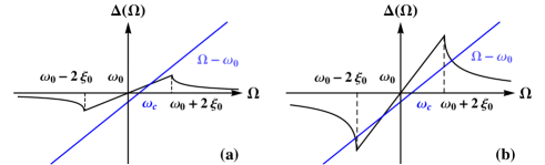
Figure 2: Graphical solutions of the imaginary poles of the retarded Green function. (a) Below the critical coupling, no solution outside the branch cut. (b) Over the critical coupling, two solutions outside the branch cut.

To see explicitly the mechanism of decoherence suppression through the strong non-Markovian effect, we may look at the steady state solution of the nanocavity in the strong coupling regime. Consider the case the frequency of the nanocavity equals to the band center of the reservoir, i.e. $\omega_{c}=\omega_{0}$, the steady state solution of $u(t)$ becomes

$$u_{\text{st}}(t)=A(\eta)e^{-i\omega_{0}t}\cos{[\omega(\eta)t]}\ .$$ (15)

This shows that the retarded Green function is enveloped by the cosine function with the amplitude $A(\eta)=\frac{\eta^{2}-2}{\eta^{2}-1}$ and the frequency $\omega(\eta)=\frac{\eta^{2}}{\sqrt{\eta^{2}-1}}\xi_{0}$ which corresponds to the energy exchange between the cavity and the reservoir. Fig. 3 shows the exact numerical result of the retarded Green function $u(t)$ [see Fig. 3(a)] and the normalized thermal fluctuation $v(t)/\bar{n}(\omega_{0},T)$ [i.e. Fig. 3(b)] in different coupling strength. Note that when the coupling $\eta>\eta_{c}=\sqrt{2}$, both the retarded Green function $u(t)$ and the thermal fluctuation $v(t)$ keep oscillating rather than damping. The oscillation indicates that the cavity keeps exchanging photons with the waveguide due to the strong non-Markovian back-reaction from the reservoir.

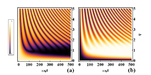
Figure 3: (a) The exact numerical result of the retarded Green function $u(t)$ and (b) the thermal fluctuation $v(t)/\bar{n}(\omega_{0},T)$ in different coupling strength. The frequency of the nanocavity $\omega_{c}$ is set to be the same as the band center of the waveguide $\omega_{0}$.

The steady solution of the fringe visibility function of Eq. (II) at zero temperature simply becomes

$$F(\alpha,t)=\exp{\{-2|\alpha|^{2}(1-A(\eta)^{2}\cos^{2}{[\omega(\eta)t]}\}}\ .$$ (16)

Instead of full decoherence, the cat state keeps oscillating in the strong coupling regime. The stronger the coupling strength is, the larger the degree of coherence can be maintained. Fig. 4 shows the periodic motion of the Wigner function for the cat state with the coupling $\eta=4$ and the temperature $T=0.5$mK. As shown in Fig. 4, the interference of the cat state keeps oscillation in time.

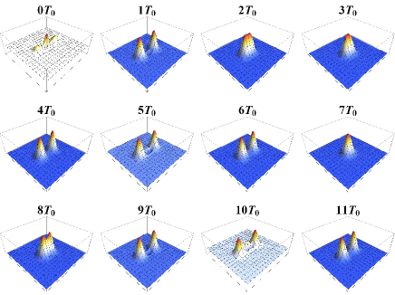
Figure 4: Time evolution of the Wigner function of the mesoscopic superposition state. The coupling strength $\eta=4$ and the cavity frequency equals to the band center of the waveguide $\omega_{c}=\omega_{0}$, $T_{0}=2\pi/\omega_{0}$. A movie for the above non-Markovian time evolution is given in sm .

In fact, in the weak coupling regime, the fringe visibility will eventually decay to $e^{-2|\alpha|^{2}}$ because of the decoherence induced by the reservoir. Then all the coherence information of the cat state will be lost. At the same time, the larger the initial temperature of the reservoir is, the faster the decoherence processes. According to (8b), as the the retarded Green function decays to zero, the two peaks of the Wigner function gradually spiral to the origin (see the movie for this Markovian time evolution given in sm ) and the thermal fluctuation $v(t)$ saturates to the equilibrium value $\bar{n}(\omega_{0},T)$ due to energy relaxation. The cat state finally decays to a thermal state with the Wigner function

$$W(z,t\rightarrow\infty)=\frac{2}{\pi[1+\bar{n}(\omega_{0},T)]}\exp{[-\frac{2|z|^{2}}{1+\bar{n}(\omega_{0},T)}]}\ .$$ (17)

In contrast, as shown in the previous analysis, when the coupling strength exceeds the critical coupling $\eta_{c}$, the decoherence dynamics of the cavity field is totally suppressed. The fringe visibility, after a short time decay, oscillates above the value of $e^{-2|\alpha|^{2}}$ for all the time. In other words, the coherence of the cat state goes to dead and birth repeatedly. In addition, according to Eq. (8b) and the stationary solution of Eq. (15) in the strong coupling regime, the two peaks of the Wigner function would keeps spiralling in and out of the origin with the frequency $\frac{\eta^{2}}{\sqrt{\eta^{2}-1}}\xi_{0}$ due to the energy exchange between the system and the reservoir, see the movie for this non-Markovian time evolution in sm . Thus, the cavity field would never be thermalized by the reservoir and the decoherence of the system is significantly suppressed.

V Conclusion

In conclusion, we have shown through the exact master equation that the nonequilibrium retarded Green function can completely determine decoherence dynamics. From analytic properties of the retarded Green function, we provided a general mechanism of decoherence suppression through the strong non-Markovian back-reaction from environments. In particular, when the coupling between the system and the reservoir exceeds a critical coupling, the bounded modes (the imaginary poles of the retarded Green function) leads to a dissipationless dynamics such that decoherence can be largely suppressed, as a strong non-Markovian memory effect. This generic behavior is explicitly demonstrated through the decoherence dynamics of the cat state. Since the nonequilibrium retarded Green function is well-defined for arbitrary open quantum system, the mechanism presented in this work should also be applicable to other more complicated open systems.

- (1) H. M. Wiseman and G. J. Milburn, Phys. Rev. Lett. 70, 548 (1993).
- (2) D. A. Lidar, I. L. Chuang, and K. B. Whaley, Phys. Rev. Lett. 81, 2594 (1998); L.-A. Wu and D. A. Lidar, Phys. Rev. Lett. 88, 207902 (2002).
- (3) L. Viola, E. Knill, and S. Lloyd, Phys. Rev. Lett. 82, 2417 (1999).
- (4) K. Khodjasteh, D. A. Lidar, Phys. Rev. Lett. 95, 180501 (2005); L. F. Santos, and L. Viola, Phys. Rev. Lett. 97, 150501 (2006); W. Yao, R. B. Liu,and L. J. Sham, Phys. Rev. Lett. 98, 077602 (2007).
- (5) G. S. Uhrig, Phys. Rev. Lett. 98, 100504 (2007); W. Yang and R. B. Liu, Phys. Rev. Lett. 101, 180403 (2008).
- (6) J. F. Du, X. Rong, N. Zhao, Y. Wang, J. Yang and R. B. Liu, Nature (London) 461, 1265 (2009); G. de Lange, Z. H. Wang, D. Riste, V. V. Dobrovitski and R. Hanson, Science 330, 60 (2010).
- (7) T. Niemczyk, F. Deppe, H. Huebl, E. P. Menzel, F. Hocke, M. J. Schwarz, Nat. Phys. 6, 772 (2010).
- (8) J. D. Thompson, B. M. Zwick, A. M. Jayich, Florian Marquardt, S. M. Girvin, and J. G. E. Harris, Nature (London) 452, 72 (2008).
- (9) C. J. Myatt, B. E. King, Q. A. Turchette, C. A. Sackett, D. Kielpinski, W. M. Itano, C. Monroe and D. J. Wineland, Nature (London) 403, 269 (2000).
- (10) M. Notomi, E. Kuramochi, and T. Tanabe, Nat. Photonics 2, 741 (2008).
- (11) H. N. Xiong, W. M. Zhang, X. Wang and M. H. Wu, Phys. Rev. A 82, 012105 (2010).
- (12) M. H. Wu, C. U Lei, W. M. Zhang and H. N. Xiong, Opt. Express 18, 18407 (2010).
- (13) M. W. Y. Tu and W. M. Zhang, Phys. Rev. B 78, 235311 (2008).
- (14) C. Monroe, D. M. Meekhof, B. E. King, and D. J. Wineland, Science 272, 1131 (1996); A. Ourjoumtsev, H. Jeong, R. Tualle-Brouri and P. Grangier, Nature (London) 448, 784 (2007).
- (15) B. M. Garraway, Phys. Rev. A 55, 2290 (1997).
- (16) H. P. Breuer, B. Kappler, and F. Petruccione, Phys. Rev. A, 59 1633 (1999); also see H. P Breuer and F. Petruccione, The Theory of Open Quantum Systems (Oxford University Press, Oxford, 2002).
- (17) C. Cohen-Tannoudji, J. Dupont-Roc, and G. Grynberg, Atom-Photon Interactions (Wiley, New York, 1992).
- (18) A. G. Kofman, G. Kurizki and B. Sherman, J. Mod. Opt. 41, 353 (1994).
- (19) S. Longhi, Phys. Rev. A 74, 063826 (2006).
- (20) C. U Lei and W. M. Zhang, arXiv:1011.4570.
- (21) See Supplemental Material in which we give two movies for the Markovian and non-Markovian time evolutions of the cat state in the weak and strong coupling regimes, respectively.